Modeling Hydrologic Change: Statistical Methods - Chapter 3 pdf
Bạn đang xem bản rút gọn của tài liệu. Xem và tải ngay bản đầy đủ của tài liệu tại đây (477.29 KB, 18 trang )
Statistical Hypothesis
Testing
3.1 INTRODUCTION
In the absence of a reliable theoretical model, empirical evidence is often an alter-
native for decision making. An intermediate step in decision making is reducing a
set of observations on one or more random variables to descriptive statistics. Exam
-
ples of frequently used descriptive statistics include the moments (i.e., mean and
variance) of a random variable and the correlation coefficient of two random variables.
Statistical hypothesis testing is a tool for making decisions about descriptive
statistics in a systematic manner. Based on concepts of probability and statistical
theory, it provides a means of incorporating the concept of risk into the assessment
of alternative decisions. More importantly, it enables statistical theory to assist in
decision making. A systematic analysis based on theoretical knowledge inserts a
measure of objectivity into the decision making.
It may be enlightening to introduce hypothesis testing in terms of populations
and samples. Data are measured in the field or in a laboratory. These represent
samples of data, and descriptive statistics computed from the measured data are
sample estimators. However, decisions should be made using the true population,
which unfortunately is rarely known. When using the empirical approach in decision
making, the data analyst is interested in extrapolating from a data sample the
statements about the population from which the individual observations that make
up the sample were obtained. Since the population is not known, it is necessary to
use the sample data to identify a likely population. The assumed population is then
used to make predictions or forecasts. Thus, hypothesis tests combine statistical
theory and sample information to make inferences about populations or parameters
of a population. The first step is to formulate hypotheses that reflect the alternative
decisions.
Because of the inherent variability in a random sample of data, a sample statistic
will usually differ from the corresponding parameter of the underlying population.
The difference cannot be known for a specific sample because the population is not
known. However, theory can suggest the distribution of the statistic from which
probability statements can be made about the difference. The difference between
the sample and population values is assumed to be the result of chance, and the
degree of difference between a sample value and the population value is a reflection
of the sampling variation. Rarely does the result of a pre-election day poll match
exactly the election result, even though the method of polling may adhere to the
proper methods of sampling. The margin of error is the best assessment of the sampling
3
© 2003 by CRC Press LLC
variation. As another example, one would not expect the mean of five random-grab
samples of the dissolved oxygen concentration in a stream to exactly equal the true
mean dissolved-oxygen concentration. Some difference between a sample estimate
of the mean and the population mean should be expected. Although some differences
may be acceptable, at some point the difference becomes so large that it is unlikely
to be the result of chance. The theoretical basis of a hypothesis test allows one to
determine the difference that is likely to result from chance, at least within the
expectations of statistical theory.
If a sufficiently large number of samples could be obtained from a population
and the value of the statistic of interest computed for each sample, the characteristics
(i.e., mean, variance, probability density function) of the statistic could be estimated
empirically. The mean of the values is the expected value. The variance of the values
indicates the sampling error of the statistic. The probability function defines the
sampling distribution of the statistic. Knowledge of the sampling distribution of the
parameter provides the basis for making decisions. Fortunately, the theoretical sam
-
pling distributions of many population parameters, such as the mean and variance,
are known from theoretical models, and inferences about these population parameters
can be made when sampled data are available to approximate unknown values of
parameters.
Given the appropriate hypotheses and a theoretical model that defines sampling
distribution, an investigator can select a decision rule that specifies sample statistics
likely to arise from the sampling distribution for each hypothesis included in the
analysis. The theoretical sampling distribution is thus used to develop the probability
statements needed for decision making.
Example 3.1
Consider Table 3.1. The individual values were sampled randomly from a standard
normal population that has a mean of 0 and a standard deviation of 1. The values
vary from −3.246 to 3.591. While many of the 200 values range from −1 to +1, a
good portion fall outside these
bounds.
The data are divided into 40 samples of 5, and the 40 means, standard deviations,
and variances are computed for each sample of 5 (see Tables 3.2, 3.3, and 3.4,
respectively). Even though the population mean is equal to 0.0, none of the 40 sample
means is the same. The 40 values show a range from −0.793 to +1.412. The sample
values vary with the spread reflective of the sampling variation of the mean. Simi
-
larly, the sample standard deviations (Table 3.3) and variances (Table 3.4) show
considerable variation; none of the values equals the corresponding population value
of 1. Again, the variation of the sample values reflects the sampling variation of the
statistics. The basic statistics question is whether or not any of the sample statistics
(e.g., mean, standard deviation, variance) are significantly different from the true
population values that are known. The answer requires knowledge of basic concepts
of
statistical theory.
Theory indicates that the mean of a sample of values drawn from a normal
population with mean µ and standard deviation on σ has an underlying normal
population with mean µ and standard deviation
. Similarly, statistical theory
σ
/ n
© 2003 by CRC Press LLC
TABLE 3.1
Forty Random Samples of Five Observations on a Standard Normal
Distribution, N(0, 1)
0.048 1.040 −0.111 −0.120 1.396 −0.393 −0.220 0.422 0.233 0.197
−0.521 −0.563 −0.116 −0.512 −0.518 −2.194 2.261 0.461 −1.533 −1.836
−1.407 −0.213 0.948 −0.073 −1.474 −0.236 −0.649 1.555 1.285 −0.747
1.822 0.898 −0.691 0.972 −0.011 0.517 0.808 2.651 −0.650 0.592
1.346 −0.137 0.952 1.467 −0.352 0.309 0.578 −1.881 −0.488 −0.329
0.420 −1.085 −1.578 −0.125 1.337 0.169 0.551 −0.745 −0.588 1.810
−1.760 −1.868 0.677 0.545 1.465 0.572 −0.770 0.655 −0.574 1.262
−0.959 0.061 −1.260 −0.573 −0.646 −0.697 −0.026 −1.115 3.591 −0.519
0.561 −0.534 −0.730 −1.172 −0.261 −0.049 0.173 0.027 1.138 0.524
−0.717 0.254 0.421 −1.891 2.592 −1.443 −0.061 −2.520 −0.497 0.909
−2.097 −0.180 −1.298 −0.647 0.159 0.769 −0.735 −0.343 0.966 0.595
0.443 −0.191 0.705 0.420 −0.486 −1.038 −0.396 1.406 0.327 1.198
0.481 0.161 −0.044 −0.864 −0.587 −0.037 −1.304 −1.544 0.946 −0.344
−2.219 −0.123 −0.260 0.680 0.224 −1.217 0.052 0.174 0.692 −1.068
1.723 −0.215 −0.158 0.369 1.073 −2.442 −0.472 2.060 −3.246 −1.020
−0.937 1.253 0.321 −0.541 −0.648 0.265 1.487 −0.554 1.890 0.499
−0.568 −0.146 0.285 1.337 −0.840 0.361 −0.468 0.746 0.470 0.171
−1.717 −1.293 −0.556 −0.545 1.344 0.320 −0.087 0.418 1.076 1.669
−0.151 −0.266 0.920 −2.370 0.484 −1.915 −0.268 0.718 2.075 −0.975
2.278 −1.819 0.245 −0.163 0.980 −1.629 −0.094 −0.573 1.548 −0.896
TABLE 3.2
Sample Means
0.258 0.205 0.196 0.347 −0.246 −0.399 0.556 0.642 −0.231 −0.425
−0.491 −0.634 −0.694 −0.643 0.897 −0.290 −0.027 −0.740 0.614 0.797
−0.334 −0.110 −0.211 −0.008 0.077 −0.793 −0.571 0.351 −0.063 −0.128
−0.219 −0.454 0.243 −0.456 0.264 −0.520 0.114 0.151 1.412 0.094
TABLE 3.3
Sample Standard Deviations
1.328 0.717 0.727 0.833 1.128 1.071 1.121 1.682 1.055 0.939
0.977 0.867 1.151 0.938 1.333 0.792 0.481 1.209 1.818 0.875
1.744 0.155 0.717 0.696 0.667 1.222 0.498 1.426 1.798 1.001
1.510 1.184 0.525 1.321 0.972 1.148 0.783 0.665 0.649 1.092
© 2003 by CRC Press LLC
indicates that if S
2 is the
variance of a random sample of size n taken from a normal
population that has the variance σ
2
, then:
(3.1)
is the value of a random variable that has a chi-square distribution with degrees of
freedom υ = n − 1.
Figure 3.1 compares the sample and population distributions. Figure 3.1(a)
shows the distrib
utions of the 200 sample values of the random variable z and the
standard normal distribution, which is the underlying population. For samples of
five from the stated population, the underlying distribution of the mean is also a
normal distribution with a mean of 0 but it has a standard deviation of
rather
than 1. The frequency distribution for the 40 sample means and the distribution of
the population are shown in Figure
3.1(b). Differences in the sample and population
distributions for both Figures
3.1(a) and 3.1(b) are due to sampling variation and
the relatively small samples, both the size of each sample (i.e., five) and the number
of samples (i.e., 40). As the sample size would increase towards infinity, the distri
-
bution of sample means would approach the population distribution. Figure 3.1(c)
shows the sample frequency histogram and the distribution of the underlying pop
-
ulation for the chi-square statistic of Equation 3.1. Again, the difference in the two
distributions reflects sampling variation. Samples much larger than 40 would show
less difference.
This example illustrates a fundamental concept of statistical analysis, namely
sampling variation. The example indicates that individual values of a sample statistic
can be quite unlike the underlying population value; however, most sample values
of a statistic are close to the population value.
3.2 PROCEDURE FOR TESTING HYPOTHESES
How can one decide whether a sample statistic is likely to have come from a specified
population? Knowledge of the theoretical sampling distribution of a test statistic
based on the statistic of interest can be used to test a stated hypothesis. The test of
a hypothesis leads to a determination whether a stated hypothesis is valid. Tests are
TABLE 3.4
Sample Variances
1.764 0.514 0.529 0.694 1.272 1.147 1.257 2.829 1.113 0.882
0.955 0.752 1.325 0.880 1.777 0.627 0.231 1.462 3.305 0.766
3.042 0.024 0.514 0.484 0.445 1.493 0.248 2.033 3.233 1.002
2.280 1.402 0.276 1.745 0.945 1.318 0.613 0.442 0.421 1.192
χ
σ
2
2
2
1
=
−()nS
15/
© 2003 by CRC Press LLC
FIGURE 3.1 Based on the data of Table 3.1: (a) the distribution of the random sample values;
(b) the distribution of the sample means; (c) distributions of the populations of X and the
mean
; and (d) chi-square distribution of the variance: sample and population.X
© 2003 by CRC Press LLC
available for almost every statistic, and each test follows the same basic steps. The
following six steps can be used to perform a statistical analysis of a hypothesis:
1. Formulate hypotheses.
2. Select the appropriate statistical model (theorem) that identifies the test
statistic and its distribution.
3. Specify the level of significance, which is a measure of risk.
4. Collect a sample of data and compute an estimate of the test statistic.
5. Obtain the critical value of the test statistic, which defines the region of
rejection.
6. Compare the computed value of the test statistic (step 4) with the critical
value (step 5) and make a decision by selecting the appropriate hypothesis.
Each of these six steps will be discussed in more detail in the following sections.
3.2.1 STEP 1: FORMULATION OF HYPOTHESES
Hypothesis testing represents a class of statistical techniques that are designed to
extrapolate information from samples of data to make inferences about populations.
The first step is to formulate two hypotheses for testing. The hypotheses will depend
on the problem under investigation. Specifically, if the objective is to make inferences
about a single population, the hypotheses will be statements indicating that a random
variable has or does not have a specific distribution with specific values of the
population parameters. If the objective is to compare two or more specific parame
-
ters, such as the means of two samples, the hypotheses will be statements formulated
to indicate the absence or presence of differences between two means. Note that the
hypotheses are composed of statements that involve population distributions or
parameters; hypotheses should not be expressed in terms of sample statistics.
The first hypothesis is called the null hypothesis, denoted by H
0
, and is always
formulated to indicate that a difference does not exist. The second or alternative
hypothesis is formulated to indicate that a difference does exist. Both are expressed
in terms of populations or population parameters. The alternative hypothesis is
denoted by either H
1
or H
A
. The null and alternative hypotheses should be expressed
in words and in mathematical terms and should represent mutually exclusive con
-
ditions. Thus, when a statistical analysis of sampled data suggests that the null
hypothesis should be rejected, the alternative hypothesis is assumed to be correct.
Some are more cautious in their interpretations and decide that failure to reject the
null hypothesis implies only that it can be accepted.
While the null hypothesis is always expressed as an equality, the alternative
hypothesis can be a statement of inequality (≠), less than (<), or greater than (>).
The selection depends on the problem. If standards for a water quality index indicated
that a stream was polluted when the index was greater than some value, the H
A
would be expressed as a greater-than statement. If the mean dissolved oxygen was
not supposed to be lower than some standard, the H
A
would be a less-than statement.
If a direction is not physically meaningful, such as when the mean should not be
significantly less than or significantly greater than some value, then a two-tailed
© 2003 by CRC Press LLC
inequality statement is used for H
A
. The statement of the alternative hypothesis is
important in steps 5 and 6. The three possible alternative hypotheses are illustrated
in Figure 3.2.
3.2.2 STEP 2: TEST STATISTIC AND ITS SAMPLING DISTRIBUTION
The two hypotheses of step 1 allow an equality or a difference between specified
populations or parameters. To test the hypotheses, it is necessary to identify the test
statistic that reflects the difference suggested by the alternative hypothesis. The
specific test statistic is generally the result of known statistical theory. The sample
value of a test statistic will vary from one sample to the next because of sampling
variation. Therefore, the test statistic is a random variable and has a sampling
distribution. A hypothesis test should be based on a theoretical model that defines
the sampling distribution of the test statistic and its parameters. Based on the
distribution of the test statistic, probability statements about computed sample values
may be made.
Theoretical models are available for all of the more frequently used hypothesis
tests. In cases where theoretical models are not available, approximations have usually
been developed. In any case, a model or theorem that specifies the test statistic, its
distribution, and its parameters must be identified in order to make a hypothesis test.
3.2.3 STEP 3: LEVEL OF SIGNIFICANCE
Two hypotheses were formulated in step 1; in step 2, a test statistic and its distribution
were selected to reflect the problem fo
r which the hypotheses were formulated. In
step 4, data will be collected to test the hypotheses. Before data collection, it is
necessary to provide a probabilistic framework for accepting or rejecting the null
FIGURE 3.2 Representation of the region of rejection (cross-hatched area), region of accep-
tance, and the critical value (S
α
): (a) H
A
: µ ¦ µ
0
; (b) H
A
: µ < µ
0
; (c) H
A
: µ > µ
0
.
© 2003 by CRC Press LLC
hypothesis and subsequently making a decision; the framework will reflect the
allowance for the variation that can be expected in a sample of data. Table
3.5 shows
the situations that could exist in the population, but are unknown (i.e., H
0
is true or
false) and the decisions that the data could suggest (i.e., accept or reject H
0
). The
decision table suggests two types of error:
Type I error: reject H
0
when, in fact, H
0
is true.
Type II error: accept H
0
when, in fact, H
0
is false.
These two incorrect decisions are not independent; for a given sample size, the
magnitude of one type of error increases as the magnitude of the other type of error
is decreased. While both types of errors are important, the decision process most
often considers only one of the errors, specifically the type I error.
The level of significance, which is usually the primary element of the decision
process in hypothesis testing, represents the probability of making a type I error and
is denoted by the Greek lower-case letter alpha, α. The probability of a type II error
is denoted by the Greek lower-case letter beta, β. The two possible incorrect decisions
are not independent. The level of significance should not be made exceptionally
small, because the probability of making a type II error will then be increased.
Selection of the level of significance should, therefore, be based on a rational analysis
of the physical system being studied. Specifically, one would expect the level of
significance to be different when considering a case involving the loss of human
life and a case involving minor property damage. However, the value chosen for α
is often based on convention and the availability of statistical tables; values for α
of 0.05 and 0.01 are selected frequently and the arbitrary nature of this traditional
means of specifying α should be recognized.
Because α and β are not independent, it is necessary to consider the implications
of both types of errors in selecting a level of significance. The concept of the power
of a statistical test is important when discussing a type II error. The power is defined
as the probability of rejecting H
0
when, in fact, it is false:
Power = 1 − β (3.2)
For some hypotheses, more than one theorem and test statistic are available, with
alternatives usually based on different assumptions. The theorems will produce
different powers, and when the assumptions are valid, the test that has the highest
power for a given level of significance is generally preferred.
TABLE 3.5
Decision Table for Hypothesis Testing
Situation
Decision H
0
is true H
0
is false
Accept H
0
Correct decision Incorrect decision: type II error
Reject H
0
Incorrect decision: type I error Correct decision
© 2003 by CRC Press LLC
3.2.4 STEP 4: DATA ANALYSIS
After obtaining the necessary data, the sample is used to provide an estimate of the
test statistic. In most cases, the data are also used to provide estimates of the
parameters required to define the sampling distribution of the test statistic. Many
tests require computing statistics called degrees of freedom in order to define the
sampling distribution of the test statistic.
3.2.5 STEP 5: REGION OF REJECTION
The region of rejection consists of values of the test statistic that are unlikely to
occur when the null hypothesis is true, as shown in the cross-hatched areas in
Figure
3.2. Extreme values of the test statistic are least likely to occur when the null
hypothesis is true. Thus, the region of rejection usually lies in one or both tails of
the distribution of the test statistic. The location of the region of rejection depends
on the statement of the alternative hypothesis. The region of acceptance consists of
all values of the test statistic that are likely if the null hypothesis is true.
The critical value of the test statistic is defined as the value that separates the
region of rejection from the region of acceptance. The critical value of the test
statistic depends on (1) the statement of the alternative hypothesis, (2) the distribution
of the test statistic, (3) the level of significance, and (4) characteristics of the sample
or data. These components represent the first four steps of a hypothesis test. Values of
the critical test statistics are usually given in tables.
The region of rejection may consist of values in both tails or in only one tail of
the distribution as suggested by Figure
3.2. Whether the problem is two-tailed, one-
tailed lower, or one-tailed upper will depend on the statement of the underlying
problem. The decision is not based on statistics, but rather is determined by the
nature of the problem tested. Although the region of rejection should be defined in
terms of values of the test statistic, it is often pictorially associated with an area of
the sampling distribution that is equal to the level of significance. The region of
rejection, region of acceptance, and the critical value are shown in Figure 3.2 for
both two-tailed and one-tailed tests. For a two-tailed test, it is standard practice to
define the critical values such that one-half of α is in each tail. For a symmetric
distribution, such as the normal or t, the two critical values will have the same
magnitude and different signs. For a nonsymmetric distribution such as the chi-
square, values will be obtained from the table such that one-half of α is in each tail;
magnitudes will be different.
Some computer programs avoid dealing with the level of significance as part of
the output and instead compute and print the rejection probability. The rejection
probability is the area in the tail of the distribution beyond the computed value of
the test statistic. This concept is best illustrated by way of examples. Assume a
software package is used to analyze a set of data and prints out a computed value
of the test statistic z of 1.92 and a rejection probability of 0.0274. This means that
approximately 2.74% of the area under the probability distribution of z lies beyond
a value of 1.92. To use this information for making a one-tailed upper test, the null
hypothesis would be rejected for any level of significance larger than 2.74% and
accepted for any level of significance below 2.74%. For a 5% level, H
0
is rejected,
© 2003 by CRC Press LLC
while for a 1% level of significance, the H
0
is accepted. Printing the rejection
probability places the decision in the hands of the reader of the output.
3.2.6 STEP 6: SELECT APPROPRIATE HYPOTHESIS
A decision whether to accept the null hypothesis depends on a comparison of the
computed value (step 4) of the test statistic and the critical value (step 5). The null
hypothesis is rejected when the computed value lies in the region of rejection.
Rejection of the null hypothesis implies acceptance of the alternative hypothesis.
When a computed value of the test statistic lies in the region of rejection, two
explanations are possible. The sampling procedure many have produced an extreme
value purely by chance; although this is very unlikely, it corresponds to the type I
error of Table
3.5. Because the probability of this event is relatively small, this
explanation is usually rejected. The extreme value of the test statistic may have
occurred because the null hypothesis was false; this explanation is most often
accepted and forms the basis for statistical inference.
The decision for most hypothesis tests can be summarized in a table such as the
following:
where P is the parameter tested against a standard value, P
0
; S is the computed value
of the test statistic; and S
α /2
and S
1−α /2
are the tabled values for the population and
have an area of α
/ 2 in the respective tails.
Example 3.2
Consider the comparison of runoff volumes from two watersheds that are similar in
drainage area and other important characteristics such as slope, but differ in the
extent of development. On one watershed, small pockets of land have been devel
-
oped. The hydrologist wants to know whether the small amount of development is
sufficient to increase storm runoff. The watersheds are located near each other and
are likely to experience the same rainfall distributions. While rainfall characteristics
are not measured, the total storm runoff volumes are measured.
The statement of the problem suggests that two means will be compared, one
for a developed watershed population µ
d
and one for an undeveloped watershed
population µ
µ
. The hydrologist believes that the case where µ
d
is less than µ
µ
is not
rational and prepares to test the following hypotheses:
H
0
: µ
d
= µ
µ
(3.3a)
H
A
: µ
d
> µ
µ
(3.3b)
If H
A
is Then reject H
0
if
P ≠ P
0
S > S
α /2
or S < S
1−α / 2
P < P
0
S < S
1−α
P > P
0
S > S
α
© 2003 by CRC Press LLC
A one-sided test of two means will be made, with the statement of the alternative
hypothesis determined by the problem statement.
Several theorems are available for comparing two means, and the hydrologist
will select the most appropriate one for the data expected to be collected in step 4.
For example, one theorem assumes equal variances that are unknown, while another
theorem assumes variances that are known and do not have to be equal. A third
theorem assumes unequal and unknown variances. The theorem should be specified
before the data are collected. In step 3, the level of significance needs to be specified.
The implications of the two types of error are:
Type I: Conclude that H
0
is false when it is true and wrongly assume that even
spotty development can increase runoff volumes. This might lead to the
requirement for unnecessary BMPs.
Type II: Conclude that H
0
is true when it is not and wrongly assume that spotty
development does not increase runoff volumes. This might allow increases
in runoff volumes to enter small streams and ultimately cause erosion
problems.
Assume that the local government concludes that the implications of a type II
error are more significant than those of the type I error. They would, therefore, want
to make β small, which may mean selecting a level of significance that is larger
than the traditional 5%.
While the data have not been collected, the problem statement has been trans-
formed into a research hypothesis (step 1), the relevant statistical theory has been
identified (step 2), and the risk of sampling errors has been considered (step 3). It
is generally considered incorrect experimental practice to collect and peruse the data
prior to establishing the first three steps of the test.
Step 4 is data collection. Generally, the largest sample size that is practical to
collect should be obtained. Accuracy is assumed to improve with increasing sample
size. Once the data are collected and organized, the test statistic and parameters
identified in the theorem are computed. It may also be necessary to check any
assumptions specified in the theorem. For the case of the runoff volumes, the sample
size may be limited by the number of storms that occur during the period allotted
to the experiment.
In step 5, the critical value would be obtained from the appropriate table. The
value may depend on parameters, such as the sample size, from step 4. The critical
value would also depend on the statement of the alternative hypothesis (step 1) and
the level of significance (step 3). The critical value and the statement of the alter
-
native hypothesis would define the region of rejection.
In step 6, the computed value of the test statistic is compared with the critical
value. If it lies in the region of rejection, the hydrologist might assume that the null
hypothesis is not correct and that spotty development in a watershed causes increases
in runoff volumes. The value of the level of significance would indicate the proba
-
bility that the null hypothesis was falsely rejected.
© 2003 by CRC Press LLC
3.3 RELATIONSHIPS AMONG HYPOTHESIS
TEST PARAMETERS
The purpose for using a statistical hypothesis test is to make a systematic decision.
The following four decision parameters are inherent to every hypothesis test, although
only two are generally given explicit consideration: sample size n, level of signifi
-
cance α, power of test P, and decision criterion C. Generally, n and α are the two
parameters selected for making the test, with a value of 5% often used for α.
However, any two of the four can be selected, and whenever two parameters are
specified, the other two are uniquely set. Each parameter plays a role in the decision:
n: The sample size is an indication of the accuracy of the statistic, that is, the
magnitude of its standard error, with the accuracy increasing with sample
size.
α: The probability of making a type I error decision, that is, the consumer’s
risk.
P: A measure of the probability of making a type II error decision, that is, the
producer’s risk. Note that Equation 3.2 shows the relationship between P
and β.
C: The criterion value that separates the regions of acceptance and rejection.
To understand the relationship of these four parameters, it is necessary to intro-
duce two new concepts: the region of uncertainty and the rejection hypothesis
denoted as H
r
. The decision process includes three hypotheses: null, alternative, and
rejection. The rejection hypothesis is established to reflect the condition where the
null hypothesis is truly incorrect and should be rejected. The null and rejection
hypotheses can be represented by probability density functions. The region between
the distribution of the test statistic when H
0
is true and the distribution when H
r
is
true is the region of uncertainty (see Figur
e 3.3).
FIGURE 3.3 Relationship between type I and II errors and critical test statistic C.
α
β
Distribution for
H
C
µ
µ
mean
Region of uncertainty
r
N
n
:
,
µµ
µ
σ
=
2
20
2
Distribution for
H
0 0
0
N
n
:
,
µµ
µ
σ
=
© 2003 by CRC Press LLC
Consider the case of a hypothesis test on a mean against some standard µ
0
, with
the null hypothesis H
0
: µ = µ
0 and t
he one-tailed alternative hypothesis, H
A
: µ < µ
0
.
If this hypothesis is true, then the test statistic is normally distributed with mean µ
0
and standard deviation , where σ is the population standard deviation, which
is assumed to be known. This means that, if H
0 is true, a sample v
alue of the mean
is likely to fall within the distribution shown on the right side in Figure
3.3. If the
null hypothesis is false and the rejection hypothesis H
r
: µ = µ
2
is true, then the test
statistic has a normal distribution with mean µ
2
and standard deviation . This
means that, if H
r
is true, a sample value of the mean is likely to fall within the
distribution shown on the left side in Figure
3.3. The region between µ
0
and µ
2
is
the region of uncertainty.
If H
0
is correct and the mean has the distribution shown on the right, then the
level of significance indicates a portion of the lower tail where type I errors are most
likely to occur. If the H
r
rejection hypothesis is correct, then the value of β indicates
the portion of the distribution for H
r
where type II errors are most likely to occur,
which is in the upper tail of the H
r
distribution. The variation within each of the two
distributions depends on the sample size, with the spread decreasing as the sample
size is increased. This reflects the greater confidence in the computed value of the
mean as the sample size increases. The cross-hatched area indicated with α repre
-
sents the probability that the null hypothesis should be rejected if H
0
is true. The
cross-hatched area indicated with β reflects the probability that the null hypothesis
will be accepted when the mean is distributed by the H
r
distribution. The decision
criterion C, which serves as the boundary for both the α and β regions, is the value
of the test statistic below which a computed value will indicate rejection of the null
hypothesis.
As indicated, when two of the four parameters are set, values for the other two
parameters are uniquely established. Each of the four parameters has statistical
implications and a physical-system association. The statistical implications of the
parameters follow:
n: A measure of the error variance of the statistical parameter, with the variance
decreasing as the sample size increases.
C: The separation line between the regions of acceptance and rejection.
α: The probability of a type I error.
β: The probability of a type II error and a measure of the statistical power of
the test (see Equation 3.2).
The physical implications of the four parameters are:
n: The quantity of empirical evidence that characterizes the underlying pop-
ulation of the test statistic.
C: The decision criterion in units of the decision variable.
α: The consumer’s risk of a wrong decision.
β: The producer’s risk of a wrong decision.
σ
/ n
σ
/ n
© 2003 by CRC Press LLC
Consider the case where n and C are set. If µ
0
, µ
2
, and σ are known based on
the characteristics of the physical system, then α and β, both shown in Figure
3.3,
are determined as follows:
(3.4a)
(3.4b)
As an alternative, if C and β are the unknowns, then they are determined by:
(3.5a)
(3.5b)
Note that Figure 3.3 could be restructured, as when the region of rejection is for a
one-tailed upper test; in this case, the normal distribution of µ for the rejection
hypothesis H
2 w
ould be to the right of the normal distribution for H
0
.
Example 3.3
Consider the hypothetical case of a state that wants to establish a criterion on a water
pollutant. A small sample is required, with the exact size set by practicality and cost
concerns. Assume that five independent grab samples are considered cost effective
and sufficiently accurate for making decisions. Extensive laboratory tests suggest
that the variation in five measurements in conditions similar to those where the test
will be applied is ±0.2 mg/L. State water quality specialists believe that conditions
are acceptably safe at 2.6 mg/L but problems occur when the concentration begins
to exceed 3.0 mg/L. They require the test on the mean to use a 5% level of
significance. Based on these conditions, they seek to determine the decision criterion
C to be used in the field and the type II error probability.
Figure 3.4 shows the normal distributions for the null hypothesis H
0
: µ = 2.6
mg/L and the rejection hypothesis H
r
: µ = 3.0 mg/L. A one-sided test is appropriate,
with H
A
: µ > 2.6 mg/L because it is not a relevant pollution problem if the level of
the pollutant is below the safe concentration of 2.6 mg/L. The distribution of the
mean for the null hypothesis is N(2.6, 0.2/
). Therefore, the decision criterion can
be calculated by:
(3.6)
αµ
µ
σ
=< =<
−
PCH Pz
C
n
(| )
/
0
0
is true
βµ
µ
σ
=> =>
−
PCH Pz
C
n
(| )
/
2
2
is true
Czn=+
µσ
0
(/ )
βµ
µ
σ
=> =>
−
PCH Pz
C
n
(| )
/
2
2
is true
Czn=+ = + =
µσ
α
0
2 6 1 645 0 2 5 2 747(/). .(./).mg/L
© 2003 by CRC Press LLC
Therefore, the probability of a type II error is found from:
(3.7)
Consequently, the state establishes the guideline that five samples are to be taken
and the null hypothesis is rejected if the mean of the sample of five exceeds 2.75
mg/L. Note that since the criterion C of 2.75 is slightly larger than 2.747, α is
theoretically slightly below 5% and β is slightly above 0.23%.
3.4 PARAMETRIC AND NONPARAMETRIC TESTS
A parametric test is based on theory or concepts that require specific conditions
about the underlying population and/or its parameters from which sample informa
-
tion will be obtained. For example, it might assume that the sample data are drawn
from a normal population or that the variance of the population is known. The
accuracy of decisions based on parametric tests depends on the extent to which these
assumptions are met. Parametric tests also require that the random variable on which
the values are measured be at least on an interval scale. Parametric tests cannot be
applied with data measured on the nominal or ordinal scale.
A nonparametric test is based on theory or concepts that have not required the
sample data to be drawn from a certain population or have conditions placed on the
parameters of the population. Nonparametric tests, in contrast to parametric tests,
do not require that the random variables be measured on the interval or ratio scales.
Many nonparametric tests are applicable to random variables measured on the
nominal or ordinal scale, and very often the nonparametric tests require that interval-
scale measurements be transformed to ranks. This does not mean that the application
of nonparametric tests makes no assumptions about the data. Many nonparametric
tests make assumptions such as data independence or that the random variable is
continuously distributed. The primary difference between the assumptions made for
the two classes of tests is that those made for nonparametric tests are not as restrictive
FIGURE 3.4 Distributions of the mean.
N
n
N
0
µ
σ
,
.,
.
26
02
5
N
2.6 3.0
mean
n
N
µ
σ
2
30
02
5
,
.,
.
βµ µ
=< = =<
−
=<− =PPzPz(.| )
./
(.).2 747 3
2 747 3 0
02 5
2 829 0 0023
2
mg / L
© 2003 by CRC Press LLC
as those made for parametric tests, such as complete specification of the underlying
population.
3.4.1 DISADVANTAGES OF NONPARAMETRIC TESTS
Nonparametric tests have applicability to a wide variety of situations and, therefore,
represent an important array of statistical decision tools. However, they have a few
disadvantages.
1. Many nonparametric test statistics are based on ranks or counts, which
are often integers. Unlike test statistics that are continuously distributed,
rank-based statistics are discrete, and therefore, it is not possible to obtain
critical values for exact levels of significance, such as 5% or 1%. Alter
-
natively, parametric test statistics are continuously distributed and critical
values for specific levels of significance can be obtained.
Consider the following hypothetical example. Assume that the test
statistic T can only take on integer values, and small values (i.e., near
zero) are unlikely to occur if the null hypothesis is true. Assume that the
cumulative probability distribution F(T) for small values of T is as follows:
If a 5% level of significance was of interest and a rejection probability
greater than 5% was considered undesirable, then a critical value of 2
would need to be used. Unfortunately, this will provide a decision that is
conservative with respect to T because use of a value of 2 indicates that
the probability of a type I error is 2.1%. If a value of 3 were used for T,
then the rejection probability would be 6.4%, which would mean that the
test would not meet the desired 5% criterion. Similarly, if a 1% rejection
probability were of interest, a critical value of 2 could not be used, but a
critical value of 1 would yield a smaller than desired rejection probability.
2. Using ranks or integer scores often results in tied values. These are more
troublesome to deal with in nonparametric tests than in parametric tests.
Ties are much rarer with continuously distributed random variables. For
some nonparametric tests, dealing with ties is not straightforward, with
several alternatives having been proposed. In some cases, the method of
handling ties distorts the rejection probability.
3. The most common criticism of nonparametric tests is that if the assump-
tions underlying a parametric alternative are met, the parametric test will
always be more powerful statistically than the nonparametric test. This is
a valid criticism, but the counterargument states that it is difficult to know
whether the assumptions underlying the parametric alternative have been
met, and if they have not been met, the nonparametric test may, in reality,
be the better test.
T 0 1 2 3 4
F(T ) 0.003 0.008 0.021 0.064 0.122
© 2003 by CRC Press LLC
3.4.2 ADVANTAGES OF NONPARAMETRIC TESTS
1. Small samples are common and in such cases, the assumptions of a
parametric test must be met exactly in order for the decision to be accurate.
Since it is extremely difficult to evaluate the extent to which parametric
test assumptions have been met, nonparametric tests are generally pre
-
ferred for cases of small sample sizes.
2. While parametric tests are limited to random variables on interval or ratio
scales, nonparametric tests can be used for random variables measured
on nominal and ordinal scales. When measurement on an interval scale
is highly imprecise, nonparametric tests may yield more accurate deci
-
sions than parametric alternatives.
3. It is easier to detect violations of the assumptions of a nonparametric test
than it is to detect violations for parametric tests. The assumptions for
nonparametric tests are usually less stringent and play a smaller role in
calculation of the test statistic.
4. When assumptions of the parametric test are violated, the level of signif-
icance used to make the decision will not be a precise measure of the
rejection probability. However, since nonparametric tests are less depen
-
dent on the adequacy of the assumptions, the probabilities are usually
exact.
3.5 PROBLEMS
3-1 What are the characteristics of a null hypothesis and an alternative hypoth-
esis?
3-2 Why is it necessary to state the null hypothesis as a finding of no signif-
icant difference (i.e., an equality) when the objective of the research may
be to show a difference?
3-3 Why are hypotheses stated in terms of the population parameters rather
than sample values?
3-4 What four factors influence the critical value of a test statistic? Show
pictorially how each factor affects the critical value.
3-5 Define the region of rejection in the following terms:
(a) Values of the test statistic
(b) Proportions of the area of the probability density function of the test
statistic
(c) The region of acceptance
(d) The critical value(s) of the test statistic
3-6 What factors contribute to sample variation? Discuss the effect of each
factor on the magnitude of the sampling variation.
3-7 Graphical analyses show the sampling distribution of the mean for samples
of 25 drawn from a normal population with µ = 8 and σ
2
= 1.2. Is it likely
that a sample of 25 from this population would have a mean of 9? Explain.
3-8 If a sample of 9 has a standard deviation of 3, it is likely that the sample
is from a normal population with a variance of 3? Explain.
© 2003 by CRC Press LLC
3-9 From a research standpoint, why should the first three steps of a hypothesis
test be made before data are collected and reviewed?
3-10 Distinguish between the sampling distribution of the random variable and
the sampling distribution of the test statistic in the various steps of a
hypothesis test.
3-11 Develop one-tailed upper, one-tailed lower, and two-tailed hypotheses
related to the hydrologic effects of afforestation.
3-12 Develop one-tailed upper, one-tailed lower, and two-tailed hypotheses
related to hydrologic effects of clearing vegetation from a stream channel.
3-13 Assume that the following null hypothesis needs to be tested: H
0
: the
mean stream scour rate of a restored stream is the same as the mean rate
prior to stream restoration. What is an appropriate alternative hypothesis?
What are the implications of type I and type II errors?
3-14 Assume that the following null hypothesis needs to be tested: H
0
: the average
baseflow from a small forested watershed is the same as the average
baseflow from an agricultural watershed. What is an appropriate alterna
-
tive hypothesis? What are the implications of type I and type II errors?
3-15 What is wrong with always using a 5% level of significance for hypothesis
testing related to watershed change?
3-16 Discuss why it might be best to conclude that a decision cannot be made
when the rejection probability is in the range from 1% to 5%.
3-17 What nonstatistical factors should be considered in setting a level of
significance?
3-18 Explain the distribution for H
r
: µ = µ2 of Figure 3.3. What is its impli-
cation with respect to sample values of the random variable and the test
statistic?
3-19 Discuss the advantages of nonparametric and parametric tests.
© 2003 by CRC Press LLC