Modeling Hydrologic Change: Statistical Methods - Chapter 5 doc
Bạn đang xem bản rút gọn của tài liệu. Xem và tải ngay bản đầy đủ của tài liệu tại đây (739.88 KB, 36 trang )
Statistical Frequency
Analysis
5.1 INTRODUCTION
Univariate frequency analysis is widely used for analyzing hydrologic data, including
rainfall characteristics, peak discharge series, and low flow records. It is primarily
used to estimate exceedance probabilities and variable magnitudes. A basic assumption
of frequency analysis is that the vector of data was measured from a temporally or
spatially homogeneous system. If measured data are significantly nonhomogeneous,
the estimated probabilities or magnitudes will be inaccurate. Thus, changes such as
climate or watershed alterations render the data unfit for frequency analysis and other
modeling methods.
If changes to the physical processes that influence the data are suspected, the
data vector should be subjected to statistical tests to decide whether the nonsta-
tionarity is significant. If the change had a significant effect on the measured data,
it may be necessary to adjust the data before subjecting it to frequency analysis.
Thus, the detection of the effects of change, the identification of the nature of any
change detected, and the appropriate adjustment of the data are prerequisite steps
required before a frequency model can be used to make probability or magnitude
estimates.
5.2 FREQUENCY ANALYSIS AND SYNTHESIS
Design problems such as the delineation of flood profiles require estimates of
discharge rates. A number of methods of estimating peak discharge rates are available.
They fall into two basic groups, one used at sites where gaged stream-flow records
are available (gaged) and the other at sites where such records are not available
(ungaged).
Statistical frequency analysis is the most common procedure for the analysis of
flood data at a gaged location. It is a general procedure that can be applied to any
type of data. Because it is so widely used with flood data, the method is sometimes
designated
flood frequency analysis
. However, statistical frequency analysis can also
be applied to other hydrologic variables such as rainfall data for the development
of intensity-duration-frequency curves and low-flow discharges for use in water
quality control. The variable could also be the mean annual rainfall, the peak
discharge, the 7-day low flow, or a water quality parameter. Therefore, the topic will
be treated in both general and specific terms.
5
L1600_Frame_C05 Page 77 Friday, September 20, 2002 10:12 AM
© 2003 by CRC Press LLC
5.2.1 P
OPULATION
VERSUS
S
AMPLE
In frequency modeling, it is important to distinguish between the population and the
sample. Frequency modeling is a statistical method that deals with a single random
variable and thus is classified as a univariate method. The goal of univariate predic-
tion is to make estimates of probabilities or magnitudes of random variables. A first
step is to identify the population. The objective of univariate data analysis is to use
sample information to determine the appropriate population density function, with
the probability density function (PDF) being the univariate model from which proba-
bility statements can be made. The input requirements for frequency modeling
include a data series and a probability distribution assumed to describe the occurrence
of the random variable. The data series could include the largest instantaneous peak
discharge to occur each year of the record. The probability distribution could be the
normal distribution. Analysis is the process of using the sample information to
estimate the population. The population consists of a mathematical model that is a
function of one or more parameters. For example, the normal distribution is a function
of two parameters: the mean
µ
and standard deviation
σ
. In addition to identifying
the correct PDF, it is necessary to quantify the parameters of the PDF. The population
consists of both the probability distribution function and the parameters.
A frequently used procedure called the
method of moments
equates characteris-
tics of the sample (e.g., sample moments) to characteristics of the population (e.g.,
population parameters). It is important to note that estimates of probability and
magnitudes are made using the assumed population and not the data sample; the
sample is used only in identifying and verifying the population.
5.2.2 A
NALYSIS
VERSUS
S
YNTHESIS
As with many hydrologic methods that have statistical bases, the terms
analysis
and
synthesis
apply to the statistical frequency method. Frequency analysis is “breaking
down” data in a way that leads to a mathematical or graphical model of the rela-
tionship between flood magnitude and its probability of occurrence. Conversely,
synthesis refers to the estimation of (1) a value of the random variable
X
for some
selected exceedance probability or (2) the exceedance probability for a selected value
of the random variable
X
. In other words, analysis is the derivation of a model that
can represent the relation between a random variable and its likelihood of occurrence,
while synthesis is using the resulting relation for purposes of estimation.
It is important to point out that frequency analysis may actually be part of a
more elaborate problem of synthesis. Specifically, separate frequency analyses can
be performed at a large number of sites within a region and the value of the random
variable
X
for a selected exceedance probability determined for each site; these values
can then be used to develop a regression model using the random variable
X
as the
criterion or dependent variable. As an example, regression equations that relate
peak discharges of a selected exceedance probability for a number of sites to water-
shed characteristics are widely used in hydrologic design. This process is called
regionalization
. These equations are derived by (1) making a frequency analysis of
annual maximum discharges at a number (
n
)
of stream gage stations in a region;
L1600_Frame_C05 Page 78 Friday, September 20, 2002 10:12 AM
© 2003 by CRC Press LLC
(2) selecting the value of the peak discharge from each of the
n
frequency curves
for a selected exceedance probability, say the l00-year flood; and (3) developing
the regression equation relating the
n
values of peak discharge to watershed char-
acteristics for the same
n
watersheds.
5.2.3 P
ROBABILITY
P
APER
Frequency analysis is a common task in hydrologic studies. A frequency analysis
usually produces a graph of the value of a single hydrologic variable versus the
probability of its occurrence. The computed graph represents the best estimate of
the statistical population from which the sample of data was drawn.
Since frequency analyses are often presented graphically, a special type of graph
paper, which is called probability paper, is required. The paper has two axes. The
ordinate is used to plot the value of the random variable, that is, the magnitude, and
the probability of its occurrence is given on the abscissa. The probability scale will
vary depending on the probability distribution used. In hydrology, the normal and
Gumbel extreme-value distributions are the two PDFs used most frequently to define
the probability scale. Figure 5.1 is on normal probability paper. The probability scale
represents the cumulative normal distribution. The scale at the top of the graph is
the exceedance probability, that is, the probability that the random variable will be
equaled or exceeded in one time period. It varies from 99.99% to 0.01%. The lower
scale is the nonexceedance probability, which is the probability that the correspond-
ing value of the random variable will not be exceeded in any one time period. This
scale extends from 0.01% to 99.99%. The ordinate of probability paper is used for
FIGURE 5.1
Frequency curve for a normal population with
µ
=
5 and
σ
=
1.
L1600_Frame_C05 Page 79 Friday, September 20, 2002 10:12 AM
© 2003 by CRC Press LLC
the random variable, such as peak discharge. The example shown in Figure 5.1 has
an arithmetic scale. Lognormal probability paper is also available, with the scale for
the random variable in logarithmic form. Gumbel and log-Gumbel papers can also
be obtained and used to describe the probabilistic behavior of random variables that
follow these probability distributions.
A frequency curve provides a probabilistic description of the likelihood of
occurrence or nonoccurrence of a variable. Figure 5.1 shows a frequency curve, with
the value of the random variable
X
versus its probability of occurrence. The upper
probability scale gives the probability that
X
will be exceeded in one time period,
while the lower probability scale gives the probability that
X
will not be exceeded.
For the frequency curve of Figure 5.1, the probability that
X
will be greater than 7
in one time period is 0.023 and the probability that
X
will not be greater than 7 in
one time period is 0.977.
Although a unique probability plotting paper could be developed for each prob-
ability distribution, papers for the normal and extreme value distributions are the
most frequently used. The probability paper is presented as a cumulative distribution
function. If the sample of data is from the distribution function used to scale the
probability paper, the data will follow the pattern of the population line when properly
plotted on the paper. If the data do not follow the population line, then (1) the sample
is from a different population or (2) sampling variation produced a nonrepresentative
sample. In most cases, the former reason is assumed, especially when the sample
size is reasonably large.
5.2.4 M
ATHEMATICAL
M
ODEL
As an alternative to a graphical solution using probability paper, a frequency analysis
may be conducted using a mathematical model. A model that is commonly used in
hydrology for normal, lognormal, and log-Pearson Type III analyses has the form
(5.1)
in which
X
is the value of the random variable having mean and standard deviation
S
, and
K
is a frequency factor. Depending on the underlying population, the specific
value of
K
reflects the probability of occurrence of the value
X
. Equation 5.1 can
be rearranged to solve for
K
when
X
, , and
S
are known and an estimate of the
probability of
X
occurring is necessary:
(5.2)
In summary, Equation 5.1 is used when the probability is known and an estimation
of the magnitude is needed, while Equation 5.2 is used when the magnitude is known
and the probability is needed.
XXKS=+
X
X
K
XX
S
=
−
L1600_Frame_C05 Page 80 Friday, September 20, 2002 10:12 AM
© 2003 by CRC Press LLC
5.2.5 P
ROCEDURE
In a broad sense, frequency analysis can be divided into two phases: deriving the
population curve and plotting the data to evaluate the goodness of fit. The following
procedure is often used to derive the frequency curve to represent the population:
1. Hypothesize the underlying density function.
2. Obtain a sample and compute the sample moments.
3. Equate the sample moments and the parameters of the proposed density
function.
4. Construct a frequency curve that represents the underlying population.
This procedure is referred to as method-of-moments estimation because the sample
moments are used to provide numerical values for the parameters of the assumed
population. The computed frequency curve representing the population can then be
used to estimate magnitudes for a given return period or probabilities for specified
values of the random variable. Both the graphical frequency curve and the mathe-
matical model of Equation 5.1 are the population.
It is important to recognize that it is not necessary to plot the data points in
order to make probability statements about the random variable. While the four steps
listed above lead to an estimate of the population frequency curve, the data should
be plotted to ensure that the population curve is a good representation of the data.
The plotting of the data is a somewhat separate part of a frequency analysis; its
purpose is to assess the quality of the fit rather than act as a part of the estimation
process.
5.2.6 S
AMPLE
M
OMENTS
For the random variable
X
, the sample mean ( ), standard deviation (
S
), and stan-
dardized skew (
g
) are, respectively, computed by:
(5.3a)
(5.3b)
(5.3c)
X
X
n
X
i
i
n
=
=
∑
1
1
S
n
XX
i
i
n
=
−
−
=
∑
1
1
2
1
05
()
.
g
nXX
nnS
i
i
n
=
−
−−
=
∑
()
()( )
3
1
3
12
L1600_Frame_C05 Page 81 Friday, September 20, 2002 10:12 AM
© 2003 by CRC Press LLC
For use in frequency analyses where the skew is used, Equation 5.3c represents a
standardized value of the skew. Equations 5.3 can also be used when the data are
transformed by taking the logarithms. In this case, the log transformation should be
done before computing the moments.
5.2.7 P
LOTTING
P
OSITION
F
ORMULAS
It is important to note that it is not necessary to plot the data before probability
statements can be made using the frequency curve; however, the data should be
plotted to determine how well they agree with the fitted curve of the assumed
population. A rank-order method is used to plot the data. This involves ordering
the data from the largest event to the smallest event, assigning a rank of 1 to the
largest event and a rank of
n
to the smallest event, and using the rank (
i
)
of the
event to obtain a probability plotting position; numerous plotting position formulas
are available. Bulletin l7B (Interagency Advisory Committee on Water Data, 1982)
provides the following generalized equation for computing plotting position prob-
abilities:
(5.4)
where
a
and
b
are constants that depend on the probability distribution. An example
is
a
=
b
=
0 for the uniform distribution. Numerous formulas have been proposed,
including the following:
Weibull: (5.5a)
Hazen: (5.5b)
Cunnane: (5.5c)
in which
i
is the rank of the event,
n
is the sample size, and
p
i
values give the
exceedance probabilities for an event with rank
i.
The data are plotted by placing a
point for each value of the random variable at the intersection of the value of the
random variable and the value of the exceedance probability at the top of the graph.
The plotted data should approximate the population line if the assumed population
model is a reasonable assumption. The various plotting position formulas provide
different probability estimates, especially in the tails of the distributions. The fol-
lowing summary shows computed probabilities for each rank for a sample of nine
using the plotting position formulas of Equations 5.5.
P
ia
nan
i
=
−
−−+1
P
i
n
i
=
+1
P
i
n
i
n
i
=
−
=
−21
2
05.
P
i
n
i
=
−
+
04
02
.
.
L1600_Frame_C05 Page 82 Friday, September 20, 2002 10:12 AM
© 2003 by CRC Press LLC
The Hazen formula gives smaller probabilities for all ranks than the Weibull and
Cunnane formulas. The probabilities for the Cunnane formula are more dispersed
than either of the others. For a sample size of 99, the same trends exist as for
n
=
9.
5.2.8 R
ETURN
P
ERIOD
The concept of return period is used to describe the likelihood of flood magnitudes.
The return period is the reciprocal of the exceedance probability, that is,
p
=
1/
T
.
Just as a 25-year rainfall has a probability of 0.04 of occurring in any one year, a
25-year flood has a probability of 0.04 of occurring in any one year. It is incorrect
to believe that a 25-year event will not occur again for another 25 years. Two 25-
year events can occur in consecutive years. Then again, a period of 100 years may
pass before a second 25-year event occurs.
Does a 25-year rainfall cause a 25-year flood magnitude? Some hydrologic
models make this assumption; however, it is unlikely to be the case in actuality. It
is a reasonable assumption for modeling because models are based on the average
of expectation or on-the-average behavior. In actuality, a 25-year flood magnitude
will not occur if a 25-year rainfall occurs on a dry watershed. Similarly, a 50-year
flood could occur from a 25-year rainfall if the watershed was saturated. Modeling
often assumes that a
T
-year rainfall on a watershed that exists in a
T
-year hydrologic
condition will produce a
T
-year flood.
5.3 POPULATION MODELS
Step 1 of the frequency analysis procedure indicates that it is necessary to select a
model to represent the population. Any probability distribution can serve as the
model, but the lognormal and log-Pearson Type III distributions are the most widely
used in hydrologic analysis. They are introduced subsequent sections, along with
the normal distribution or basic model.
n
=
9
n
=
99
Rank
p
w
p
h
p
c
Rank
p
w
p
h
p
c
1 0.1 0.05 0.065 1 0.01 0.005 0.006
2 0.2 0.15 0.174 2 0.02 0.015 0.016
3 0.3 0.25 0.283 .
4 0.4 0.35 0.391 .
5 0.5 0.45 0.500 .
6 0.6 0.55 0.609 98 0.98 0.985 0.984
7 0.7 0.65 0.717 99 0.99 0.995 0.994
8 0.8 0.75 0.826
9 0.9 0.85 0.935
L1600_Frame_C05 Page 83 Friday, September 20, 2002 10:12 AM
© 2003 by CRC Press LLC
5.3.1 NORMAL DISTRIBUTION
Commercially available normal probability paper is commonly used in hydrology.
Following the general procedure outlined above, the specific steps used to develop
a curve for a normal population are as follows:
1. Assume that the random variable has a normal distribution with population
parameters
µ
and
σ
.
2. Compute the sample moments and S (the skew is not needed).
3. For normal distribution, the parameters and sample moments are related
by
µ
= and
σ
= S.
4. A curve is fitted as a straight line with plotted at an exceedance
probability of 0.8413 and at an exceedance probability of 0.1587.
The frequency curve of Figure 5.1 is an example for a normal distribution with a
mean of 5 and a standard deviation of 1. It is important to note that the curve passes
through the two points: and . It also passes through
the point defined by the mean and a probability of 0.5. Two other points that could
be used are and . Using the points farther
removed from the mean has the advantage that inaccuracies in the line drawn to
represent the population will be smaller than when using more interior points.
The sample values should then be plotted (see Section 5.2.7) to decide whether
the measured values closely approximate the population. If the data provide a
reasonable fit to the line, one can assume that the underlying population is the normal
distribution and the sample mean and standard deviation are reasonable estimates
of the location and scale parameters, respectively. A poor fit indicates that the normal
distribution is not appropriate, that the sample statistics are not good estimators of
the population parameters, or both.
When using a frequency curve, it is common to discuss the likelihood of events
in terms of exceedance frequency, exceedance probability, or the return period (T)
related to the exceedance probability (p) by p = l/T, or T = l/p. Thus, an event with
an exceedance probability of 0.01 should be expected to occur 1 time in 100. In
many cases, a time unit is attached to the return period. For example, if the data
represent annual floods at a location, the basic time unit is 1 year. The return period
for an event with an exceedance probability of 0.01 would be the l00-year event
(i.e., T = 1/0.01 = 100); similarly, the 25-year event has an exceedance probability
of 0.04 (i.e., p = 1/25 = 0.04). It is important to emphasize that two T-year events
will not necessarily occur exactly T years apart. They can occur in successive years
or may be spaced three times T years apart. On average, the events will be spaced
T years apart. Thus, in a long period, say 10,000 years, we would expect 10,000/T
events to occur. In any single 10,000-year period, we may observe more or fewer
occurrences than the mean (10,000/T).
Estimation with normal frequency curve — For normal distribution, estimation
may involve finding a probability corresponding to a specified value of the random
variable or finding the value of the random variable for a given probability. Both
problems can be solved using graphical analysis or the mathematical models of
X
X
()XS−
()XS+
(, .)XS− 0 8413
(, .)XS+ 0 1587
(,.)XS+ 2 0 0228
(, .
)
XS− 2 0 9772
L1600_Frame_C05 Page 84 Friday, September 20, 2002 10:12 AM
© 2003 by CRC Press LLC
Equations 5.1 and 5.2. A graphical analysis estimation involves simply entering the
probability and finding the corresponding value of the random variable or entering
the value of the random variable and finding the corresponding exceedance proba-
bility. In both cases, the fitted line (population) is used. The accuracy of the estimated
value will be influenced by the accuracy used in drawing the line or graph.
Example 5.1
Figure 5.2 shows a frequency histogram for the data in Table 5.1. The sample consists
of 58 annual maximum instantaneous discharges, with a mean of 8620 ft
3
/sec, a
standard deviation of 4128 ft
3
/sec, and a standardized skew of 1.14. In spite of the
large skew, the normal frequency curve was fitted using the procedure of the pre-
ceding section. Figure 5.3 shows the cumulative normal distribution using the sample
mean and the standard deviation as estimates of the location and scale parameters.
The population line was drawn by plotting X + S = 12,748 at p = 15.87% and –
S = 4492 at p = 84.13%, using the upper scale for the probabilities. The data were
plotted using the Weibull plotting position formula (Equation 5.5a). The data do not
provide a reasonable fit to the population; they show a significant skew with an
FIGURE 5.2 Frequency histograms of the annual maximum flood series (solid line) and
logarithms (dashed line) based on mean (and for logarithms) and standard deviations (S
x
and
for logarithms S
y
): Piscataquis River near Dover-Foxcroft, Maine.
X
L1600_Frame_C05 Page 85 Friday, September 20, 2002 10:12 AM
© 2003 by CRC Press LLC
TABLE 5.1
Frequency Analysis of Peak Discharge Data:
Piscataquis River
Rank
Weibull
Probability
Random
Variable
Logarithm of
Variable
1 0.0169 21500 4.332438
2 0.0339 19300 4.285557
3 0.0508 17400 4.240549
4 0.0678 17400 4.240549
5 0.0847 15200 4.181844
6 0.1017 14600 4.164353
7 0.1186 13700 4.136721
8 0.1356 13500 4.130334
9 0.1525 13300 4.123852
10 0.1695 13200 4.120574
11 0.1864 12900 4.110590
12 0.2034 11600 4.064458
13 0.2203 11100 4.045323
14 0.2373 10400 4.017034
15 0.2542 10400 4.017034
16 0.2712 10100 4.004322
17 0.2881 9640 3.984077
18 0.3051 9560 3.980458
19 0.3220 9310 3.968950
20 0.3390 8850 3.946943
21 0.3559 8690 3.939020
22 0.3729 8600 3.934499
23 0.3898 8350 3.921686
24 0.4068 8110 3.909021
25 0.4237 8040 3.905256
26 0.4407 8040 3.905256
27 0.4576 8040 3.905256
28 0.4746 8040 3.905256
29 0.4915 7780 3.890980
30 0.5085 7600 3.880814
31 0.5254 7420 3.870404
32 0.5424 7380 3.868056
33 0.5593 7190 3.856729
34 0.5763 7190 3.856729
35 0.5932 7130 3.853090
36 0.6102 6970 3.843233
37 0.6271 6930 3.840733
38 0.6441 6870 3.836957
39 0.6610 6750 3.829304
40 0.6780 6350 3.802774
41 0.6949 6240 3.795185
L1600_Frame_C05 Page 86 Friday, September 20, 2002 10:12 AM
© 2003 by CRC Press LLC
TABLE 5.1
Frequency Analysis of Peak Discharge Data:
Piscataquis River (Continued)
Rank
Weibull
Probability
Random
Variable
Logarithm of
Variable
42 0.7119 6200 3.792392
43 0.7288 6100 3.785330
44 0.7458 5960 3.775246
45 0.7627 5590 3.747412
46 0.7797 5300 3.724276
47 0.7966 5250 3.720159
48 0.8136 5150 3.711807
49 0.8305 5140 3.710963
50 0.8475 4710 3.673021
51 0.8644 4680 3.670246
52 0.8814 4570 3.659916
53 0.8983 4110 3.613842
54 0.9153 4010 3.603144
55 0.9322 4010 3.603144
56 0.9492 3100 3.491362
57 0.9661 2990 3.475671
58 0.9831 2410 3.382017
Mean 8620 3.889416
Standard deviation 4128 0.203080
Standardized skew 1.14 −0.066
FIGURE 5.3 Piscataquis River near Dover-Foxcroft, Maine.
L1600_Frame_C05 Page 87 Friday, September 20, 2002 10:12 AM
© 2003 by CRC Press LLC
especially poor fit to the tails of the distribution (i.e., high and low exceedance
probabilities). Because of the poor fit, the line shown in Figure 5.3 should not be
used to make probability statements about the future occurrences of floods; for
example, the normal distribution (i.e., the line) suggests a 1% chance flood magnitude
of slightly more than 18,000 ft
3
/sec. However, if a line was drawn subjectively
through the trend of the points, the flood would be considerably larger, say about
23,000 ft
3
/sec.
The 100-year flood is estimated by entering with a probability of 1% and finding
the corresponding flood magnitude. Probabilities can be also estimated. For example,
if a levee system at this site would be overtopped at a magnitude of 16,000 ft
3
/sec,
the curve indicates a corresponding probability of about 4%, which is the 25-year
flood.
To estimate probabilities or flood magnitudes using the mathematical model,
Equation 5.1 becomes X = + zS because the frequency factor K of Equation 5.1
becomes the standard normal deviate z for a normal distribution, where values of z
are from Appendix Table A.1. To find the value of the random variable X, estimates
of
and S must be known and the value of z obtained from Appendix Table A.1
for any probability. To find the probability for a given value of the random variable
X, Equation 5.2 is used to solve for the frequency factor z (which is K in Equation 5.2);
the probability is then obtained from Table A.1 using the computed value of z. For
example, the value of z from Table A.1 for a probability of 0.01 (i.e., the 100-year
event) is 2.327; thus, the flood magnitude is:
which agrees with the value obtained from the graphical analysis. For a discharge
of 16,000 ft
3
/sec, the corresponding z value is:
Appendix Table A.1 indicates the probability is 0.0377, which agrees with the
graphical estimate of about 4%.
5.3.2 LOGNORMAL DISTRIBUTION
When a poor fit to observed data is obtained, a different distribution function should
be considered. For example, when the data demonstrate a concave, upward curve,
as in Figure 5.3, it is reasonable to try a lognormal distribution or an extreme value
distribution. It may be preferable to fit with a distribution that requires an estimate
of the skew coefficient, such as a log-Pearson Type III distribution. However, sample
estimates of the skew coefficient may be inaccurate for small samples.
The same procedure used for fitting the normal distribution can be used to fit
the lognormal distribution. The underlying population is assumed to be lognormal.
The data must first be transformed to logarithms, Y = log X. This transformation
X
X
XXzS=+ = + =8620 2 327 4128 18 226. ( ) . /sec ft
3
z
XX
S
=
−
=
−
=
16 000 8 620
4 128
1 788
,,
,
.
L1600_Frame_C05 Page 88 Friday, September 20, 2002 10:12 AM
© 2003 by CRC Press LLC
creates a new random variable Y. The mean and standard deviation of the logarithms
are computed and used as the parameters of the population; it is important to recognize
that the logarithm of the mean does not equal the mean of the logarithms, which is
also true for the standard deviation. Thus, the logarithms of the mean and standard
deviation should not be used as parameters; the mean and standard deviation of the
logarithms should be computed and used as the parameters. Either natural or base-
10 logarithms may be used, although the latter is more common in hydrology. The
population line is defined by plotting the straight line on arithmetic probability paper
between the points ( + S
y
, 0.1587) and ( − S
y
, 0.8413), where and S
y
are the
mean and standard deviation of the logarithms, respectively. In plotting the data,
either the logarithms can be plotted on an arithmetic scale or the untransformed data
can be plotted on a logarithmic scale.
When using a frequency curve for a lognormal distribution, the value of the
random variable Y and the moments of the logarithms ( and S
y
) are related by the
equation:
(5.6)
in which z is the value of the standardized normal variate; values of z and corre-
sponding probabilities can be found in Table A.1. Equation 5.6 can be used to
estimate either flood magnitudes for a given exceedance probability or an exceedance
probability for a specific discharge. To find a discharge for a specific exceedance
probability the standard normal deviate z is obtained from Table A.1 and used in
Equation 5.6 to compute the discharge. To find the exceedance probability for a
given discharge Y, Equation 5.6 is rearranged by solving for z. With values of Y, ,
and S
y
, a value of z is computed and used with Table A.1 to compute the exceedance
probability. Of course, the same values of both Y and the probability can be obtained
directly from the frequency curve.
Example 5.2
The peak discharge data for the Piscataquis River were transformed by taking the
logarithm of each of the 58 values. The moments of the logarithms are as follows:
= 3.8894, S
y
= 0.20308, and g = −0.07. Figure 5.4 is a histogram of the logarithms.
In comparison to the histogram of Figure 5.2, the logarithms of the sample data are
less skewed. While a skew of −0.07 would usually be rounded to −0.1, it is sufficiently
close to 0 such that the discharges can be represented with a lognormal distribution.
The frequency curve is shown in Figure 5.5. To plot the lognormal population curve,
the following two points were used: − S
y
= 3.686 at p = 84.13% and + S
y
=
4.092 at p = 15.87%. The data points were plotted on Figure 5.5 using the Weibull
formula and show a much closer agreement with the population line in comparison
to the points for the normal distribution in Figure 5.3. It is reasonable to assume
that the measured peak discharge rates can be represented by a lognormal distribution
and that the future flood behavior of the watershed can be described statistically
using a lognormal distribution.
Y Y Y
Y
YYzS
y
=+
Y
Y
Y Y
L1600_Frame_C05 Page 89 Friday, September 20, 2002 10:12 AM
© 2003 by CRC Press LLC
If one were interested in the probability that a flood of 20,000 ft
3
/sec would be
exceeded in a given year, the logarithm of 20,000 (4.301) would be entered on the
discharge axis and followed to the assumed population line. Reading the exceedance
probability corresponding to that point on the frequency curve, a flood of 20,000
ft
3
/sec has a 1.7% chance of being equaled or exceeded in any one year. It can also
FIGURE 5.4 Histogram of logarithms of annual maximum series: Piscataquis River.
FIGURE 5.5 Frequency curve for the logarithms of the annual maximum discharge.
L1600_Frame_C05 Page 90 Friday, September 20, 2002 10:12 AM
© 2003 by CRC Press LLC
be interpreted that over the span of 1,000 years, a flood discharge of 20,000 ft
3
/sec
would be exceeded in 17 of those years; it is important to understand that this is an
average. In any period of 1,000 years, a value of 20,000 ft
3
/sec may be exceeded or
reached less frequently than in 17 of the 1,000 years, but on average 17 exceedances
would occur in 1,000 years.
The probability of a discharge of 20,000 ft
3
/sec can also be estimated mathe-
matically. The standard normal deviate is
(5.7a)
The value of z is entered into Table A.1, which yields a probability of 0.9786. Since
the exceedance probability is of interest, this is subtracted from 1, which yields a
value of 0.0214. This corresponds to a 47-year flood. The difference between the
mathematical estimate of 2.1% and the graphical estimate of 1.7% is due to the error
in the graph. The computed value of 2.1% should be used.
The frequency curve can also be used to estimate flood magnitudes for selected
probabilities. Flood magnitude is found by entering the figure with the exceedance
probability, moving vertically to the frequency curve, and finally moving horizontally
to flood magnitude. For example, the 100-year flood for the Piscataquis River can
be found by starting with an exceedance probability of 1%, moving to the curve of
Figure 5.5 and then to the ordinate, which indicates a logarithm of about 4.3586 or
a discharge of 22,800 ft
3
/sec. Discharges for other exceedance probabilities can be
found that way or by using the mathematical model of Equation 5.1. In addition to
the graphical estimate, Equation 5.6 can be used to obtain a more exact estimate.
For an exceedance probability of 0.01, a z value of 2.327 is obtained from Table A.1.
Thus, the logarithm is
(5.7b)
Taking the antilogarithm yields a discharge of 23,013 ft
3
/sec.
5.3.3 LOG-PEARSON TYPE III DISTRIBUTION
Normal and lognormal frequency analyses were introduced because they are easy
to understand and have a variety of uses. The statistical distribution most commonly
used in hydrology in the United States is the log-Pearson Type III (LP3) because it
was recommended by the U.S. Water Resources Council in Bulletin 17B (Interagency
Advisory Committee on Water Data, 1982). The Pearson Type III is a PDF. It is
widely accepted because it is easy to apply when the parameters are estimated using
the method of moments and it usually provides a good fit to measured data. LP3
analysis requires a logarithmic transformation of data; specifically, the common
logarithms are used as the variates, and the Pearson Type III distribution is used as
the PDF.
z
Y
S
y
=
−
=
−
=
log( , ) . .
.
.
20 000 4 301 3 8894
0 20308
2 027
YYzS
y
=+ = + =3 8894 2 327 0 20308 4 3620 (.).
L1600_Frame_C05 Page 91 Friday, September 20, 2002 10:12 AM
© 2003 by CRC Press LLC
While LP3 analyses have been made for most stream gage sites in the United
States and can be obtained from the U.S. Geological Survey, a brief description of
the analysis procedure is provided here. Although the method of analysis presented
here will follow the procedure recommended by the Water Resources Council, you
should consult Bulletin 17B when performing an analysis because a number of
options and adjustments cited in the bulletin are not discussed here. This section
only provides sufficient detail so that a basic frequency analysis can be made and
properly interpreted.
Bulletin l7B provides details for the analysis of three types of data: a systematic
gage record, regional data, and historic information for the site. The systematic
record consists of the annual maximum flood record. It is not necessary for the
record to be continuous as long as the missing part of the record is not the result of
flood experience, such as the destruction of the stream gage during a large flood.
Regional information includes a generalized skew coefficient, a weighting procedure
for handling independent estimates, and a means of correlating a short systematic
record with a longer systematic record from a nearby stream gaging station. Historic
records, such as high-water marks and newspaper accounts of flooding that occurred
before installation of the gage, can be used to augment information at the site.
The procedure for fitting an LP3 curve with a measured systematic record is
similar to the procedure used for the normal and lognormal analyses described earlier.
The steps of the Bulletin 17B procedure for analyzing a systematic record based on
a method-of-moments analysis are as follows:
1. Create a series that consists of the logarithms Y
i
of the annual maximum
flood series x
i
.
2. Using Equations 5.3 compute the sample mean, , standard deviation,
S
y
, and standardized skew, g
s
, of the logarithms created in step 1.
3. For selected values of the exceedance probability (p), obtain values of the
standardized variate K from Appendix Table A.5 (round the skew to the
nearest tenth).
4. Determine the values of the LP3 curve for the exceedance probabilities
selected in Step 3 using the equation
(5.8)
in which y is the logarithmic value of the LP3 curve.
5. Use the antilogarithms of the Y
j
values to plot the LP3 frequency curve.
After determining the LP3 population curve, the data can be plotted to determine
adequacy of the curve. The Weibull plotting position is commonly used. Confidence
limits can also be placed on the curve; a procedure for computing confidence
intervals is discussed in Bulletin 17B. In step 3, it is necessary to select two or more
points to compute and plot the LP3 curve. If the absolute value of the skew is small,
the line will be nearly straight and only a few points are necessary to draw it
accurately. When the absolute value of the skew is large, more points must be used
Y
YYKS
y
=+
L1600_Frame_C05 Page 92 Friday, September 20, 2002 10:12 AM
© 2003 by CRC Press LLC
because of the greater curvature. When selecting exceedance probabilities to compute
the LP3 curve, it is common to include 0.5, 0.2, 0.1, 0.04, 0.02, 0.01, and 0.002
because these correspond to return periods that are usually of interest.
Example 5.3
Data for the Back Creek near Jones Springs, West Virginia (USGS gaging station
016140), are given in Table 5.2. Based on the 38 years of record (1929–1931 and
1939–1973), the mean, standard deviation, and skew of the common logarithms are
3.722, 0.2804, and −0.731, respectively; the skew will be rounded to −0.7. Table 5.3
shows the K values of Equation 5.8 for selected values of the exceedance probability
(p); these values were obtained from Table A.5 using p and the sample skew of −0.7.
Equation 5.8 was used to compute the logarithms of the LP3 discharges for the
selected exceedance probabilities (Table 5.3).
The logarithms of the discharges were then plotted versus the exceedance prob-
abilities, as shown in Figure 5.6. The rank of each event is also shown in Table 5.2
and was used to compute the exceedance probability using the Weibull plotting
position formula (Equation 5.4a). The logarithms of the measured data were plotted
versus the exceedance probability (Figure 5.6). The data show a reasonable fit to the
frequency curve, although the fit is not especially good for the few highest and the
lowest measured discharges; the points with exceedance probabilities between 80%
and 92% suggest a poor fit. Given that we can only make subjective assessments of
FIGURE 5.6 Log-Pearson Type III frequency curve for Back Creek near Jones Spring, West
Virginia, with station skew () and weighted skew (- - -).
L1600_Frame_C05 Page 93 Friday, September 20, 2002 10:12 AM
© 2003 by CRC Press LLC
TABLE 5.2
Annual Maximum Floods for Back Creek
Year Q Log Q Rank p
1929 8750 3.9420 7 0.179
1930 15500 4.1903 3 0.077
1931 4060 3.6085 27 0.692
1939 6300 3.7993 14 0.359
1940 3130 3.4955 35 0.897
1941 4160 3.6191 26 0.667
1942 6700 3.8261 12 0.308
1943 22400 4.3502 1 0.026
1944 3880 3.5888 30 0.769
1945 8050 3.9058 9 0.231
1946 4020 3.6042 28 0.718
1947 1600 3.2041 37 0.949
1948 4460 3.6493 23 0.590
1949 4230 3.6263 25 0.641
1950 3010 3.4786 36 0.923
1951 9150 3.9614 6 0.154
1952 5100 3.7076 19 0.487
1953 9820 3.9921 5 0.128
1954 6200 3.7924 15 0.385
1955 10700 4.0294 4 0.103
1956 3880 3.5888 31 0.795
1957 3420 3.5340 33 0.846
1958 3240 3.5105 34 0.872
1959 6800 3.8325 11 0.282
1960 3740 3.5729 32 0.821
1961 4700 3.6721 20 0.513
1962 4380 3.6415 24 0.615
1963 5190 3.7152 18 0.462
1964 3960 3.5977 29 0.744
1965 5600 3.7482 16 0.410
1966 4670 3.6693 21 0.538
1967 7080 3.8500 10 0.256
1968 4640 3.6665 22 0.564
1969 536 2.7292 38 0.974
1970 6680 3.8248 13 0.333
1971 8360 3.9222 8 0.205
1972 18700 4.2718 2 0.051
1973 5210 3.7168 17 0.436
Source: Interagency Advisory Committee on Water Data,
Guidelines for Determining Flood-Flow Frequency, Bulletin
17B, U.S. Geological Survey, Office of Water Data Coordina-
tion, Reston, VA, 1982.
L1600_Frame_C05 Page 94 Friday, September 20, 2002 10:12 AM
© 2003 by CRC Press LLC
the goodness of fit, the computed frequency curve appears to be a reasonable estimate
of the population.
The curve of Figure 5.6 can be used to estimate flood discharges for selected
exceedance probabilities or exceedance probabilities for selected discharges. For
example, the 100-year flood (p = 0.01) equals 16,992 ft
3
/sec (i.e., log Q = 4.2285
from Table 5.3). The exceedance probability for a discharge of 10,000 ft
3
/sec (i.e.,
log Q = 4) is approximately 0.155 from Figure 5.6; this corresponds to the 6-year
event.
5.4 ADJUSTING FLOOD RECORD FOR URBANIZATION
A statistical flood frequency analysis is based on the assumption of a homogeneous
annual flood record. Significant changes in land use lead to nonhomogeneity of flood
characteristics, thus violating the assumptions that underline frequency analysis. A
flood frequency analysis based on a nonhomogeneous record will produce inaccurate
estimates. The effects of nonhomogeneity must be estimated before computation of
frequency analysis so that the flood record can be adjusted.
Urbanization is a primary cause of nonhomogeneity of flood records. Although
the problem has been recognized for decades, few attempts to develop a systematic
procedure for adjuisting flood records have been made. Multiparameter watershed
models have been used for this purpose; however, a single model or procedure for
adjustment has not been widely accepted by the professional community. Compar-
isons of methods for adjusting records have not been made.
5.4.1 EFFECTS OF URBANIZATION
A number of models that allow assessment of the effects of urbanization on peak
discharges are available. Some models provide bases for accounting for urbanization,
but it is difficult to develop a general statement of the effects of urbanization from
TABLE 5.3
Computation of Log-Pearson Type III
Frequency Curve for Back Creek Near
Jones Springs, West Virginia
pK+KS
y
Q(ft
3
/sec)
0.99 −2.82359 2.9303 852
0.90 −1.33294 3.3482 2,230
0.70 −0.42851 3.6018 3,998
0.50 0.11578 3.7545 5,682
0.20 0.85703 3.9623 9,169
0.10 1.18347 4.0538 11,320
0.04 1.48852 4.1394 13,784
0.02 1.66325 4.1884 15,430
0.01 1.80621 4.2285 16,922
L1600_Frame_C05 Page 95 Friday, September 20, 2002 10:12 AM
© 2003 by CRC Press LLC
these models. For example, with the rational method, urban development affects the
runoff coefficient and the time of concentration. Thus, it is not possible to make a
general statement that a 5% increase in imperviousness will cause an x% increase
in the peak discharge for a specific return period. Other models are not so constrained.
A number of regression equations are available that include the percentage of
imperviousness as a predictor variable. They make it possible to develop a general
statement on the effects of urbanization. Sarma, Delleur, and Rao (1969) provided
one such example:
(5.9)
in which A is the drainage area (mi
2
), U is the fraction of imperviousness, P
E
is the
volume of excess rainfall (in.), T
R
is the duration of rainfall excess (hours), and q
p
is the peak discharge (ft
3
/sec). Since the model has the power-model form, the
specific effect of urbanization depends on the values of the other predictor variables
(A, P
E
, and T
R
). However, the relative sensitivity of Equation 5.9 can be used as a
measure of the effect of urbanization. The relative sensitivity (S
R
) is given by:
(5.10)
Evaluation of Equation 5.10 yields a relative sensitivity of 1.516. Thus, a 1% change
in U will cause a change of 1.516% in the peak discharge. This estimate is an average
effect since it is independent of both the value of U and the return period.
Based on the work of Carter (1961) and Anderson (1970), Dunne and Leopold
(1978) provided the following equation for estimating the effect of urbanization:
f = 1 + 0.015U (5.11)
in which f is a factor that gives the relative increase in peak discharge for a percent
imperviousness of U. The following is a summary of the effect of urbanization based
on the model of Equation 5.11:
Thus, a 1% increase in U will increase the peak discharge by 1.5%, which is the
same effect shown by Equation 5.10.
The Soil Conservation Service (SCS) provided an adjustment for urbanization
for the first edition of the TR-55 (1975) chart method. The adjustment depended on
the percentages of imperviousness, the hydraulic length modified, and the runoff
curve number (CN). Although the adjustment did not specifically include return period
as a factor, the method incorporates the return period through rainfall input. Table 5.4
shows adjustment factors for imperviousness and the hydraulic length modified.
U 0 1020304050100
f 1 1.15 1.3 1.45 1.6 1.75 2.5
qAUPT
pER
=+
−
484 1 1
0 723 1 516 1 113 0 403
.()
S
q
U
U
q
R
p
p
=
∂
∂
⋅
L1600_Frame_C05 Page 96 Friday, September 20, 2002 10:12 AM
© 2003 by CRC Press LLC
Assuming that these changes occur in the same direct proportion, the effect of
urbanization on peak discharges is the square of the factor. Approximate measures
of the effect of changes in the adjustment factor from change in U are also given in
Table 5.4 (R
s
); these values of R
s
represent the change in peak discharge due to the
peak factors provided in the first edition of TR-55. Additional effects of urban
development on the peak discharge would be reflected in change in the CN. However,
the relative sensitivities of the SCS chart method suggest a change in peak discharge
of 1.3% to 2.6% for a 1% change in urbanization, which represents the combined
effect of changes in imperviousness and modifications of the hydraulic length.
USGS urban peak discharge equations (Sauer et al., 1981) provide an alternative
for assessing effects of urbanization. Figures 5.7 and 5.8 show the ratios of urban-
to-rural discharges as functions of the percentages of imperviousness and basin
development factors. For the 2-year event, the ratios range from 1 to 4.5; 4.5 indicates
complete development. For the 100-year event, the ratio has a maximum value of
2.7. For purposes of illustration and assuming basin development occurs in direct
proportion to changes in imperviousness, the values of Table 5.4 (R
s
) show the effects
of urbanization on peak discharge. The average changes in peak discharge due to a
1% change in urbanization are 1.75 and 0.9% for the 2- and 100-year events,
respectively. While the methods discussed reveal an effect of about 1.5%, the USGS
equations suggest that the effect is slightly higher for more frequent storm events
and slightly lower for less frequent events. This is generally considered rational.
Rantz (1971) devised a method for assessing the effects of urbanization on peak
discharges using simulated data of James (1965) for the San Francisco Bay area.
Urbanization is characterized by two variables: the percentages of channels sewered
and basins developed. The percentage of basins developed is approximately twice
the percentage of imperviousness. Table 5.5 shows the relative sensitivity of the peak
discharge to the percent imperviousness and the combined effect of the percentages
of channels sewered and basins developed. For urbanization as measured by the
percentage change in imperviousness, the mean relative sensitivities are 2.6%, 1.7%,
TABLE 5.4
Adjustment Factors for Urbanization
SCS Chart Method USGS Urban Equations
CN U f f
2
R
s
TUf
1
R
s
70 20 1.13 1.28 0.018 2-yr 20 1.70 0.016
25 1.17 1.37 0.019 25 1.78 0.016
30 1.21 1.46 0.025 30 1.86 0.018
35 1.26 1.59 0.026 35 1.95 0.020
40 1.31 1.72 — 40 2.05 —
80 20 1.10 1.21 0.013 100-yr 20 1.23 0.010
25 1.13 1.28 0.014 25 1.28 0.008
30 1.16 1.35 0.019 30 1.32 0.008
35 1.20 1.44 0.015 35 1.36 0.010
40 1.23 1.51 — 40 1.41 —
L1600_Frame_C05 Page 97 Friday, September 20, 2002 10:12 AM
© 2003 by CRC Press LLC
and 1.2% for the 2-, 10-, and 100-year events, respectively. These values are larger
by about 30% to 50% than the values computed from the USGS urban equations.
When both the percentages of channels sewered and basins developed are used as
indices of development, the relative sensitivities are considerably higher. The mean
relative sensitivities are 7.1, 5.1, and 3.5% for the 2-, 10-, and 100-year events, respec-
tively. These values are much larger than the values suggested by the other methods
discussed above. Thus, the effects of urbanization vary considerably, which compli-
cates the adjustment of measured flow data to produce a homogeneous flood series.
FIGURE 5.7 Ratio of the urban-to-rural 2-year peak discharge as a function of basin devel-
opment factor and impervious area.
FIGURE 5.8 Ratio of the urban-to-rural 100-year peak discharge as a function of basin devel-
opment factor and impervious area.
L1600_Frame_C05 Page 98 Friday, September 20, 2002 10:12 AM
© 2003 by CRC Press LLC
5.4.2 METHOD FOR ADJUSTING FLOOD RECORD
The literature does not identify a single method considered best for adjusting a flood
record. Each method depends on the data used to calibrate the prediction process.
The databases used to calibrate the methods are very sparse. However, the sensitiv-
ities suggest that a 1% increase in imperviousness causes an increase in peak
discharge of about 1% to 2.5% with the former value for the 100-year event and the
latter for the 2-year event. However, considerable variation is evident at any return
period.
Based on the general trends of the data, a method of adjusting a flood record
was developed. Figure 5.9 shows the peak adjustment factor as a function of the
exceedance probability for percentages of imperviousness up to 60%. The greatest
effect is for the more frequent events and the highest percentage of imperviousness.
Given the return period of a flood peak for a nonurbanized watershed, the effect of
an increase in imperviousness can be assessed by multiplying the discharge by the
peak adjustment factor for the return period and percentage of imperviousness.
Where it is necessary to adjust a discharge from a partially urbanized watershed
to a discharge for another condition, the discharge can be divided by the peak
adjustment factor for the existing condition and the resulting “rural” discharge
multiplied by the peak adjustment factor for the second watershed condition. The
first operation (division) adjusts the discharge to a magnitude representative of a
nonurbanized condition. The adjustment method of Figure 5.9 requires an exceed-
ance probability. For a flood record, the best estimate of the probability is obtained
from a plotting position formula. The following procedure can be used to adjust a
TABLE 5.5
Effect on Peak Discharge of (a) the Percentage of Imperviousness
(U) and (b) the Combined Effect of Urban Development (D)
T = 2-yr T = 10-yr T = 100-yr
fR
s
fR
s
fR
s
(a) U (%)
10 1.22 0.025 1.13 0.015 1.08 0.011
20 1.47 0.025 1.28 0.017 1.19 0.012
30 1.72 0.026 1.45 0.018 1.31 0.013
40 1.98 0.029 1.63 0.018 1.44 0.012
50 2.27 1.81 1.56
(b) D (%)
10 1.35 0.040 1.18 0.022 1.15 0.010
20 1.75 0.060 1.40 0.040 1.25 0.025
30 2.35 0.085 1.80 0.050 1.50 0.050
40 3.20 0.100 2.30 0.092 2.00 0.055
50 4.20 3.22 2.55
L1600_Frame_C05 Page 99 Friday, September 20, 2002 10:12 AM
© 2003 by CRC Press LLC
flood record for which the individual flood events have occurred on a watershed
undergoing continuous changes in levels of urbanization.
1. Identify the percentage of imperviousness for each event in the flood
record and the percentage of imperviousness for which an adjusted flood
record is needed.
2. Compute the rank (i) and exceedance probability (p) for each event in the
flood record (a plotting position formula can be used to compute the
probability).
3. Using exceedance probability and the actual percentage of impervious-
ness, find from Figure 5.9 the peak adjustment factor ( f
1
) to transform the
measured peak from the level of imperviousness to a nonurbanized con-
dition.
4. Using the exceedance probability and the percentage of imperviousness
for which a flood series is needed, find from Figure 5.9 the peak adjust-
ment factor ( f
2
) necessary to transform the nonurbanized peak to a dis-
charge for the desired level of imperviousness.
5. Compute the adjusted discharge (Q
a
) by:
(5.12)
in which Q is the measured discharge.
6. Repeat steps 3, 4, and 5 for each event in the flood record and rank the
adjusted series.
FIGURE 5.9 Peak adjustment factors for urbanizing watersheds.
Q
f
f
Q
a
=
2
1
L1600_Frame_C05 Page 100 Friday, September 20, 2002 10:12 AM
© 2003 by CRC Press LLC
7. If the ranks of the adjusted discharges differ considerably from the ranks
of the measured discharges, steps 2 through 6 should be repeated until
the ranks do not change.
This procedure should be applied to the flood peaks and not to the logarithms of the
flood peaks, even when the adjusted series will be used to compute a lognormal or log-
Pearson Type III frequency curve. The peak adjustment factors of Figure 5.9 are based
on methods that show the effect of imperviousness on flood peaks, not on the logarithms.
Example 5.4
Table 5.6 contains the 48-year record of annual maximum peak discharges for the
Rubio Wash watershed in Los Angeles. Between 1929 and 1964, the percent of
impervious cover also shown in Table 5.6 increased from 18 to 40%. The mean and
standard deviation of the logarithms of the record are 3.2517 and 0.1910, respec-
tively. The station skew was −0.53, and the map skew was −0.45. Therefore, a
weighted skew of −0.5 was used.
The procedure was used to adjust the flood record from actual levels of imper-
viousness for the period from 1929 to 1963 to current impervious cover conditions.
For example, while the peak discharges for 1931 and 1945 occurred when the percent
cover was 19% and 34%, respectively, the values were adjusted to a common percent-
age of 40%, which is the watershed state after 1964. Three iterations of adjustments
were required. The iterative process is required because the return period for some
of the earlier events changed considerably from the measured record; for example,
the rank of the 1930 peak changed from 30 to 22 on the first trial, and the rank of
the 1933 event went from 20 to 14. Because of such changes in the rank, the
exceedance probabilities change and thus the adjustment factors, which depend on
the exceedance probabilities, change. After the second adjustment is made, the rank
of the events did not change, so the process is complete. The adjusted series is given
in the last part of Table 5.6.
The adjusted series has a mean and standard deviation of 3.2800 and 0.1785,
respectively. As expected, the mean increased because earlier events occurred when
less impervious cover existed and the standard deviation decreased because the
measured data include both natural variation and variation due to different levels of
imperviousness. The adjustment corrected for the latter variation. The adjusted flood
frequency curve will generally be higher than the curve for the measured series but
will have a shallower slope. The higher curve reflects the effect of greater impervi-
ousness (40%). The lower slope reflects the single level of imperviousness of the
adjusted series. The computations for the adjusted and unadjusted flood frequency
curves are given in Table 5.7. The percent increases in the 2-, 5-, 10-, 15-, 50-, and
100-year flood magnitudes appear in Table 5.7. The change is minor because the
imperviousness did not change after 1964 and changes from 1942 to 1964 were
minor (i.e., 10%). Most larger storm events occurred after the watershed reached
developed condition. The adjusted series represents annual flooding for a constant
urbanization condition (40% imperviousness). Of course, the adjusted series is not
measured and its accuracy depends on the representativeness of Figure 5.9 for
measuring the effects of urbanization.
L1600_Frame_C05 Page 101 Friday, September 20, 2002 10:12 AM
© 2003 by CRC Press LLC