Modeling Hydrologic Change: Statistical Methods - Chapter 7 pot
Bạn đang xem bản rút gọn của tài liệu. Xem và tải ngay bản đầy đủ của tài liệu tại đây (887.33 KB, 37 trang )
Statistical Detection
of Nonhomogeneity
7.1 INTRODUCTION
Data independent of the flood record may suggest that a flood record may not be
stationary. Knowing that changes in land cover occurred during the period of record
will necessitate assessing the effect of the land cover change on the peaks in the
record. Statistical hypothesis testing is the fundamental approach for analyzing a
flood record for nonhomogeneity. Statistical testing only suggests whether a flood
record has been affected; it does not quantify the effect. Statistical tests have been
used in flood frequency and hydrologic analyses for the detection of nonhomogeneity
(Natural Environment Research Council, 1975; Hirsch, Slack, and Smith, 1982;
Pilon and Harvey, 1992; Helsel and Hirsch, 1992).
The runs test can be used to test for nonhomogeneity due to a trend or an episodic
event. The Kendall test tests for nonhomogeneity associated with a trend. Correlation
analyses can also be applied to a flood series to test for serial independence, with
significance tests applied to assess whether an observed dependency is significant;
the Pearson test and the Spearman test are commonly used to test for serial corre-
lation. If a nonhomogeneity is thought to be episodic, separate flood frequency
analyses can be done to detect differences in characteristics, with standard techniques
used to assess the significance of the differences. The Mann–Whitney test is useful
for detecting nonhomogeneity associated with an episodic event.
Four of these tests (all but the Pearson test) are classified as nonparametric. They
tests can be applied directly to the discharges in the annual maximum series without
making a logarithmic transform. The exact same solution results when the test is
applied to the logarithms and to the untransformed data with all four tests. This is
not true for the Pearson test, which is parametric. Because a logarithmic transform
is cited in Bulletin 17B (Interagency Advisory Committee on Water Data, 1982),
the transform should also be applied when making the statistical test for the Pearson
correlation coefficient.
The tests presented for detecting nonhomogeneity follow the six steps of hypoth-
esis testing: (1) formulate hypotheses; (2) identify theory that specifies the test
statistic and its distribution; (3) specify the level of significance; (4) collect the data
and compute the sample value of the test statistic; (5) obtain the critical value of
the test statistic and define the region of rejection; and (6) make a decision to reject
the null hypothesis if the computed value of the test statistic lies in the region of
rejection.
7
L1600_Frame_C07 Page 135 Friday, September 20, 2002 10:16 AM
© 2003 by CRC Press LLC
7.2 RUNS TEST
Statistical methods generally assume that hydrologic data measure random variables,
with independence among measured values. The runs (or run) test is based on the
mathematical theory of runs and can test a data sample for lack of randomness or
independence (or conversely, serial correlation) (Siegel, 1956; Miller and Freund,
1965). The hypotheses follow:
H
0
: The data represent a sample of a single independently distributed random
variable.
H
A
: The sample elements are not independent values.
If one rejects the null hypothesis, the acceptance of nonrandomness does not indicate
the type of nonhomogeneity; it only indicates that the record is not homogeneous.
In this sense, the runs test may detect a systematic trend or an episodic change. The
test can be applied as a two-tailed or one-tailed test. It can be applied to the lower
or upper tail of a one-tailed test.
The runs test is based on a sample of data for which two outcomes are possible,
x
1
or
x
2
. These outcomes can be membership in two groups, such as exceedances or
nonexceedances of a user-specified criterion such as the median. In the context of
flood-record analysis, these two outcomes could be that the annual peak discharges
exceed or do not exceed the median value for the flood record. A
run
is defined as
a sequence of one or more of outcome
x
1
or outcome
x
2
. In a sequence of
n
values,
n
1
and
n
2
indicate the number of outcomes
x
1
and
x
2
, respectively, where
n
1
+
n
2
=
n
. The outcomes are determined by comparing each value in the data series with a
user-specified criterion, such as the median, and indicating whether the data value
exceeds (
+
) or does not exceed (
−
) the criterion. Values in the sequence that equal
the median should be omitted from the sequences of
+
and
−
values. The solution
procedure depends on sample size. If the values of
n
1
and
n
2
are both less than 20,
the critical number of runs,
n
α
, can be obtained from a table. If
n
1
or
n
2
is greater
than 20, a normal approximation is made.
The theorem that specifies the test statistic for large samples is as follows: If
the ordered (in time or space) sample data, contains
n
1
and
n
2
values for the two
possible outcomes,
x
1
and
x
2
, respectively, in
n
trials, where both
n
1
and
n
2
are not
small, the sampling distribution of the number of runs is approximately normal with
mean, , and variance, , which are approximated by:
(7.1a)
and
(7.1b)
U S
u
2
U
nn
nn
=+
2
1
12
12
()
()
()( )
S
nn nn n n
nn nn
u
2
12 12 1 2
12
2
12
22
1
=
−−
++−
L1600_Frame_C07 Page 136 Friday, September 20, 2002 10:16 AM
© 2003 by CRC Press LLC
in which
n
1
+
n
2
=
n
. For a sample with
U
runs, the test statistic is (Draper and
Smith, 1966):
(7.2)
where
z
is the value of a random variable that has a standard normal distribution.
The 0.5 in Equation 7.2 is a continuity correction applied to help compensate for
the use of a continuous (normal) distribution to approximate the discrete distribution
of
U
. This theorem is valid for samples in which
n
1
or
n
2
exceeds 20.
If both
n
1
and
n
2
are less than 20, it is only necessary to compute the number
of runs
U
and obtain critical values of
U
from appropriate tables (see Appendix
Table A.5). A value of
U
less than or equal to the lower limit or greater than or
equal to the upper limit is considered significant. The appropriate section of the table
is used for a one-tailed test. The critical value depends on the number of values,
n
1
and
n
2
. The typically available table of critical values is for a 5% level of significance
when applied as a two-tailed test. When it is applied as a one-tailed test, the critical
values are for a 2.5% level of significance.
The level of significance should be selected prior to analysis. For consistency
and uniformity, the 5% level of significance is commonly used. Other significance
levels can be justified on a case-by-case basis. Since the basis for using a 5% level
of significance with hydrologic data is not documented, it is important to assess the
effect of using the 5% level on the decision.
The runs test can be applied as a one-tailed or two-tailed test. If a direction is
specified, that is, the test is one-tailed, then the critical value should be selected
accordingly to the specification of the alternative hypothesis. After selecting the
characteristic that determines whether an outcome should belong to group 1 (
+
) or
group 2 (
−
), the runs should be identified and
n
1
,
n
2
, and
U
computed. Equations
7.1a and 7.1b should be used to compute the mean and variance of
U
. The computed
value of the test statistic
z
can then be determined with Equation 7.2.
For a two-tailed test, if the absolute value of
z
is greater than the critical value
of
z
, the null hypothesis of randomness should be rejected; this implies that the
values of the random variable are probably not randomly distributed. For a one-
tailed test where a small number of runs would be expected, the null hypothesis is
rejected if the computed value of
z
is less (i.e., more negative) than the critical value
of
z
. For a one-tailed test where a large number of runs would be expected, the null
hypothesis is rejected if the computed value of
z
is greater than the critical value of
z
. For the case where either
n
l
or
n
2
is greater than 20, the critical value of
z
is
−
z
α
or
+
z
α
depending on whether the test is for the lower or upper tail, respectively.
When applying the runs test to annual maximum flood data for which watershed
changes may have introduced a systematic effect into the data, a one-sided test is
typically used. Urbanization of a watershed may cause an increase in the central
tendency of the peaks and a decrease in the coefficient of variation. Channelization
may increase both the central tendency and the coefficient of variation. Where the
primary effect of watershed change is to increase the central tendency of the annual
z
UU
S
u
=
−−05.
L1600_Frame_C07 Page 137 Friday, September 20, 2002 10:16 AM
© 2003 by CRC Press LLC
maximum floods, it is appropriate to apply the runs test as a one-tailed test with a
small number of runs. Thus, the critical
z
value would be a negative number, and
the null hypothesis would be rejected when the computed
z
is more negative than
the critical
z
α
, which would be a negative value. For a small sample test, the null
hypothesis would be rejected if the computed number of runs was smaller than the
critical number of runs.
Example 7.1
The runs test can be used to determine whether urban development caused an
increase in annual peak discharges. It was applied to the annual flood series of the
rural Nolin River and the urbanized Pond Creek watersheds to test the following
null (
H
0
) and alternative (
H
A
) hypotheses:
H
0
: The annual peak discharges are randomly distributed from 1945 to 1968,
and thus a significant trend is not present.
H
A
: A significant trend in the annual peak discharges exists since the annual
peaks are not randomly distributed.
The flood series is represented in Table 7.1 by a series of
+
and
−
symbols. The
criterion that designates a
+
or
−
event is the median flow (i.e., the flow exceeded
or not exceeded as an annual maximum in 50% of the years). For the Pond Creek
and North Fork of the Nolin River watersheds, the median values are 2175 ft
3
/sec
and 4845 ft
3
/sec, respectively (see Table 7.1). If urbanization caused an increase in
discharge rates, then the series should have significantly more
+
symbols in the part
of the series corresponding to greater urbanization and significantly more
−
symbols
before urbanization. The computed number of runs would be small so a one-tailed
TABLE 7.1
Annual Flood Series for Pond Creek (q
p
, median ==
==
2175 ft
3
/s) and the Nolin
River (Q
p
, median ==
==
4845 ft
3
/s)
Year
q
p
Sign
Q
p
Sign Year
q
p
Sign
Q
p
Sign
1945 2000
−
4390
−
1957 2290
+
6510
+
1946 1740
−
3550
−
1958 2590 + 8300 +
1947 1460 − 2470 − 1959 3260 + 7310 +
1948 2060 − 6560 + 1960 + 1640 −
1949 1530 − 5170 + 1961 + 4970 +
1950 1590 − 4720 − 1962 + 2220 −
1951 1690 − 2720 − 1963 + 2100 −
1952 1420 − 5290 + 1964 + 8860 +
1953 1330 − 6580 + 1965 + 2300 −
1954 607 − 548 − 1966 4380 + 4280 −
1955 1380 − 6840 + 1967 3220 + 7900 +
1956 1660 − 3810 − 1968 4320 + 5500 +
L1600_Frame_C07 Page 138 Friday, September 20, 2002 10:16 AM
© 2003 by CRC Press LLC
test should be applied. While rejection of the null hypothesis does not necessarily
prove that urbanization caused a trend in the annual flood series, the investigator
may infer such a cause.
The Pond Creek series has only two runs (see Table 7.1). All values before 1956
are less than the median and all values after 1956 are greater than the median. Thus,
n
l
= n
2
= 12. The critical value of 7 was obtained from Table A.5. The null hypothesis
should be rejected if the number of runs in the sample is less than or equal to 7.
Since a one-tailed test was used, the level of significance is 0.025. Because the
sequence includes only two runs for Pond Creek, the null hypothesis should be
rejected. The rejection indicates that the data are nonrandom. The increase in urban-
ization after 1956 may be a causal factor for this nonrandomness.
For the North Fork of the Nolin River, the flood series represents 14 runs (see
Table 7.1). Because n
1
and n
2
are the same as for the Pond Creek analysis, the critical
value of 7 applies here also. Since the number of runs is greater than 7, the null
hypothesis of randomness cannot be rejected. Since the two watersheds are located
near each other, the trend in the flood series for Pond Creek is probably not due to
an increase in rainfall. (In a real-world application, rainfall data should be examined
for trends as well.) Thus, it is probably safe to conclude that the flooding trend for
Pond Creek is due to urban development in the mid-1950s.
7.2.1 RATIONAL ANALYSIS OF RUNS TEST
Like every statistical test, the runs test is limited in its ability to detect the influence
of a systematic factor such as urbanization. If the variation of the systematic effect
is small relative to the variation introduced by the random processes, then the runs
test may suggest randomness. In such a case, all of the variation may be attributed
to the effects of the random processes.
In addition to the relative magnitudes of the variations due to random processes
and the effects of watershed change, the ability of the runs test to detect the effects
of watershed change will depend on its temporal variation. Two factors are important.
First, change can occur abruptly over a short time or gradually over the duration of
a flood record. Second, an abrupt change may occur near the center, beginning, or
end of the period of record. These factors must be understood when assessing the
results of a runs test of an annual maximum flood series.
Before rationally analyzing the applicability of the runs test for detecting hydro-
logic change, summarizing the three important factors is worthwhile.
1. Is the variation introduced by watershed change small relative to the
variation due to the randomness of rainfall and watershed processes?
2. Has the watershed change occurred abruptly over a short part of the length
of record or gradually over most of the record length?
3. If the watershed change occurred over a short period, was it near the
center of the record or at one of the ends?
Answers to these questions will help explain the rationality of the results of a runs
test and other tests discussed in this chapter.
L1600_Frame_C07 Page 139 Friday, September 20, 2002 10:16 AM
© 2003 by CRC Press LLC
Responses to the above three questions will include examples to demonstrate
the general concepts. Studies of the effects of urbanization have shown that the more
frequent events of a flood series may increase by a factor of two for large increases
in imperviousness. For example, the peaks in the later part of the flood record for
Pond Creek are approximately double those from the preurbanization portion of the
flood record. Furthermore, variation due to the random processes of rainfall and
watershed conditions appears relatively minimal, so the effects of urbanization are
apparent (see Figure 2.4). The annual maximum flood record for the Ramapo River
at Pompton Lakes, New Jersey (1922 through 1991) is shown in Figure 7.1. The
scatter is very significant, and an urbanization trend is not immediately evident.
Most urban development occurred before 1968, and the floods of record then appear
smaller than floods that occurred in the late 1960s. However, the random scatter
largely prevents the identification of effects of urbanization from the graph. When
the runs test is applied to the series, the computed test statistic of Equation 7.2 equals
zero, so the null hypothesis of randomness cannot be rejected. In contrast to the
series for Pond Creek, the large random scatter in the Ramapo River series masks
the variation due to urbanization.
The nature of a trend is also an important consideration in assessing the effect
of urbanization on the flows of an annual maximum series. Urbanization of the Pond
Creek watershed occurred over a short period of total record length; this is evident
in Figure 2.4. In contrast, Figure 7.2 shows the annual flood series for the Elizabeth
River, at Elizabeth, New Jersey, for a 65-year period. While the effects of the random
processes are evident, the flood magnitudes show a noticeable increase. Many floods
at the start of the record are below the median, while the opposite is true for later
years. This causes a small number of runs, with the shorter runs near the center of
record. The computed z statistic for the run test is −3.37, which is significant at the
FIGURE 7.1 Annual maximum peak discharges for Ramapo River at Pompton Lakes, New
Jersey.
20,000
18,000
16,000
14,000
12,000
10,000
8000
6000
4000
2000
0
1887 1904 1921
1938
1955
1972
1989
Peak Discharge in Cubic Feet per Second
L1600_Frame_C07 Page 140 Friday, September 20, 2002 10:16 AM
© 2003 by CRC Press LLC
0.0005 level. Thus, a gradual trend, especially with minimal variation due to random
processes, produces a significant value for the runs test. More significant random
effects may mask the hydrologic effects of gradual urban development.
Watershed change that occurs over a short period, such as that in Pond Creek,
can lead to acceptance or rejection of the null hypothesis for the runs test. When
the abrupt change is near the middle of the series, the two sections of the record
will have similar lengths; thus, the median of the series will fall in the center of the
two sections, with a characteristic appearance of two runs, but it quite possibly will
be less than the critical number of runs. Thus, the null hypothesis will be rejected.
Conversely, if the change due to urbanization occurs near either end of the record
length, the record will have short and long sequences. The median of the flows will
fall in the longer sequence; thus, if the random effects are even moderate, the flood
series will have a moderate number of runs, and the results of a runs test will suggest
randomness.
It is important to assess the type (gradual or abrupt) of trend and the location
(middle or end) of an abrupt trend. This is evident from a comparison of the series
for Pond Creek, Kentucky, and Rahway River in New Jersey. Figure 7.3 shows the
annual flood series for the Rahway River. The effect of urbanization appears in the
later part of the record. The computed z statistic for the runs test is −1.71, which is
not significant at the 5% level, thus suggesting that randomness can be assumed.
7.3 KENDALL TEST FOR TREND
Hirsch, Slack, and Smith (1982) and Taylor and Loftis (1989) provide assessments
of the Kendall nonparametric test. The test is intended to assess the randomness of
a data sequence X
i
; specifically, the hypotheses (Hirsch, Slack, and Smith, 1982) are:
FIGURE 7.2 Annual maximum peak discharges for Elizabeth River, New Jersey.
5000
4500
4000
3500
3000
2500
2000
1500
1000
500
0
1925 1936 1947
1958
1969
1980
1991
Peak Discharge in Cubic Feet per Second
L1600_Frame_C07 Page 141 Friday, September 20, 2002 10:16 AM
© 2003 by CRC Press LLC
H
0
: The annual maximum peak discharges (x
i
) are a sample of n independent
and identically distributed random variables.
H
A
: The distributions of x
j
and x
k
are not identical for all k, j ≤ n with k ≤ j.
The test is designed to detect a monotonically increasing or decreasing trend in the
data rather than an episodic or abrupt event. The above H
A
alternative is two-sided,
which is appropriate if a trend can be direct or inverse. If a direction is specified,
then a one-tailed alternative must be specified. Gradual urbanization would cause a
direct trend in the annual flood series. Conversely, afforestation can cause an inverse
trend in an annual flood series. For the direct (inverse) trend in a series, the one-
sided alternative hypothesis would be:
H
A
: A direct (inverse) trend exists in the distribution of x
j
and x
k
.
The theorem defining the test statistic is as follows. If x
j
and x
k
are independent
and identically distributed random values, the statistic S is defined as:
(7.3)
where
(7.4)
FIGURE 7.3 Annual maximum peak discharges for Rahway River, New Jersey.
6000
5400
4800
4200
3600
3000
2400
1800
1200
600
0
1925 1936 1947
1958
1969
1980
1991
Peak Discharge in Cubic Feet per Second
Sxx
j
k
jk
n
k
n
=−
=+=
−
∑∑
sgn( )
11
1
z =
>
=
−<
10
00
10
if
if
if
Θ
Θ
Θ
L1600_Frame_C07 Page 142 Friday, September 20, 2002 10:16 AM
© 2003 by CRC Press LLC
For sample sizes of 30 or larger, tests of the hypothesis can be made using the
following test statistic:
(7.5a)
in which z is the value of a standard normal deviate, n is the sample size, and V is
the variance of S, given by:
(7.5b)
in which g is the number of groups of measurements that have equal value (i.e.,
ties) and t
i
is the number of ties in group i. Mann (1945) provided the variance for
series that did not include ties, and Kendall (1975) provided the adjustment shown
as the second term of Equation 7.5b. Kendall points out that the normal approxima-
tion of Equation 7.5a should provide accurate decisions for samples as small as 10,
but it is usually applied when N ≥ 30. For sample sizes below 30, the following
τ
statistic can be used when the series does not include ties:
(7.6)
Equation 7.6 should not be used when the series includes discharges of the same
magnitude; in such cases, a correction for ties can be applied (Gibbons, 1976).
After the sample value of the test statistic z is computed with Equation 7.5 and
a level of significance
α
selected, the null hypothesis can be tested. Critical values
of Kendall’s
τ
are given in Table A.6 for small samples. For large samples with a
two-tailed test, the null hypothesis H
0
is rejected if z is greater than the standard
normal deviate z
α
/2
or less than −z
α
/2
. For a one-sided test, the critical values are z
α
for a direct trend and −z
α
for an inverse trend. If the computed value is greater than
z
α
for the direct trend, then the null hypothesis can be rejected; similarly, for an
inverse trend, the null hypothesis is rejected when the computer z is less (i.e., more
negative) than −z
α
.
Example 7.2
A simple hypothetical set of data is used to illustrate the computation of
τ
and
decision making. The sample consists of 10 integer values, as shown, with the values
of sgn(Θ) shown immediately below the data for each sample value.
z
SV S
S
SV S
=
−>
=
+<
()/
()/
.
.
10
00
10
05
05
for
for
for
V
nn n t t t
ii i
i
g
=
−+− −+
=
∑
()( ) ()( )12 5 12 5
18
1
τ
=−21Snn/[ ( )]
L1600_Frame_C07 Page 143 Friday, September 20, 2002 10:16 AM
© 2003 by CRC Press LLC
Since there are 33 + and 12 − values, S of Equation 7.3 is 21. Equation 7.6 yields
the following sample value of
τ
:
Since the sample size is ten, critical values are obtained from tables, with the
following tabular summary of the decision for a one-tailed test:
Thus, for a 5% level the null hypothesis is rejected, which suggests that the data
contain a trend. At smaller levels of significance, the test would not suggest a trend
in the sequence.
Example 7.3
The 50-year annual maximum flood record for the Northwest Branch of the Anacostia
River watershed (Figure 2.1) was analyzed for trend. Since the record length is
greater than 30, the normal approximation of Equation 7.5 is used:
(7.7)
Because the Northwest Branch of the Anacostia River has undergone urbanization,
the one-sided alternative hypothesis for a direct trend is studied. Critical values of
z for 5% and 0.1% levels of significance are 1.645 and 3.09, respectively. Thus, the
computed value of 3.83 is significant, and the null hypothesis is rejected. The test
suggests that the flood series reflects an increasing trend that we may infer resulted
from urban development within the watershed.
2503714968
+−++−++++
−−+−−+++
+++++++
+−++++
−−+−+
++++
+++
−−
+
Level of Significance Critical
ττ
ττ
Decision
0.05 0.422 Reject H
0
0.025 0.511 Accept H
0
0.01 0.600 Accept H
0
0.005 0.644 Accept H
0
τ
==
221
10 9
0 467
()
()
.
z ==
459
119 54
383
.
.
L1600_Frame_C07 Page 144 Friday, September 20, 2002 10:16 AM
© 2003 by CRC Press LLC
Example 7.4
The two 24-year, annual-maximum flood series in Table 7.1 for Pond Creek and the
North Fork of the Nolin River were analyzed for trend. The two adjacent watersheds
have the same meteorological conditions. Since the sample sizes are below 30,
Equation 7.6 will be used for the tests. S is 150 for Pond Creek and 30 for Nolin
River. Therefore, the computed
τ
for Pond Creek is:
For Nolin River, the computed
τ
is:
For levels of significance of 5, 2.5, 1, and 0.5%, the critical values are 0.239, 0.287,
0.337, and 0.372, respectively. Thus, even at a level of significance of 0.5%, the null
hypotheses would be rejected for Pond Creek. For Nolin River, the null hypothesis
must be accepted at a 5% level of significance. The results show that the Pond Creek
series is nonhomogeneous, which may have resulted from the trend in urbanization.
Since the computed
τ
of 0.109 is much less than any critical values, the series for
the North Fork of the Nolin River does not contain a trend.
7.3.1 RATIONALE OF KENDALL STATISTIC
The random variable S is used for both the Kendall
τ
of Equation 7.6 and the normal
approximation of Equation 7.5. If a sequence consists of alternating high-flow and
low-flow values, the summation of Equation 7.3 would be the sum of alternating +
1 and −1 values, such as for deforestation, which would yield a near-zero value for
S. Such a sequence is considered random so the null hypothesis should be accepted
for a near-zero value. Conversely, if the sequence consisted of a series of increasingly
larger flows, such as for deforestation, which would indicate a direct trend, then
each Θ of Equation 7.3 would be +1, so S would be a large value. If the flows
showed an inverse trend, such as for afforestation, then the summation of Equation
7.3 would consist of values of −1, so S would be a large negative value. The
denominator of Equation 7.6 is the maximum possible number for a sequence of n
flows, so the ratio of S to n(n − 1) will vary from −1, for an inverse trend to +1 for
a direct trend. A value of zero indicates the absence of a trend (i.e., randomness).
For the normal approximation of Equation 7.5, the z statistic has the form of
the standard normal transformation equation: , where the mean and
s is the standard deviation. For Equation 7.5, S is the random variable, a mean of
zero is inherent in the null hypothesis of randomness, and the denominator is the
standard deviation of S. Thus, the null hypothesis of the Kendall test is accepted for
values of z that are not significantly different from zero.
τ
=
−
=
()
()
.
150 2
24 24 1
0 543
τ
=
−
=
()
()
.
30 2
24 24 1
0 109
zxxs=−()/
x
L1600_Frame_C07 Page 145 Friday, September 20, 2002 10:16 AM
© 2003 by CRC Press LLC
The Kendall test statistic depends on the difference in magnitude between every
pair of values in the series, not just adjacent values. For a series in which an abrupt
watershed change occurred, there will be more changes in sign of the (x
j
− x
k
) value
of Equation 7.3, which will lead to a value of S that is relatively close to zero. This
is especially true if the abrupt change is near one of the ends of the flood series.
For a gradual watershed change, a greater number of positive values of (x
j
− x
k
) will
occur. Thus, the test will suggest a trend. In summary, the Kendall test may detect
watershed changes due to either gradual trends or abrupt events. However, it appears
to be more sensitive to changes that result from gradually changing trends.
7.4 PEARSON TEST FOR SERIAL INDEPENDENCE
If a watershed change, such as urbanization, introduces a systematic variation into
a flood record, the values in the series will exhibit a measure of serial correlation.
For example, if the percentage of imperviousness gradually increases over all or a
major part of the flood record, then the increase in the peak floods that results from
the higher imperviousness will introduce a measure of correlation between adjacent
flood peaks. This correlation violates the assumption of independence and station-
arity that is required for frequency analysis.
The serial correlation coefficient is a measure of common variation between
adjacent values in a time series. In this sense, serial correlation, or autocorrelation,
is a univariate statistic, whereas a correlation coefficient is generally associated with
the relationship between two variables. The computational objective of a correlation
analysis is to determine the degree of correlation in adjacent values of a time or
space series and to test the significance of the correlation. The nonstationarity of an
annual flood series as caused by watershed changes is the most likely hydrologic
reason for the testing of serial correlation. In this sense, the tests for serial correlation
are used to detect nonstationarity and nonhomogeneity. Serial correlation in a data
set does not necessarily imply nonhomogeneity.
The Pearson correlation coefficient (McNemar, 1969; Mendenhall and Sincich,
1992) can be used to measure the association between adjacent values in an ordered
sequence of data. For example, in assessing the effect of watershed change on an
annual flood series, the correlation would be between values for adjacent years in
a sequential record. The correlation coefficient could be computed for either the
measured flows or their logarithms but the use of logarithms is recommended when
analyzing annual maximum flood records. The two values will differ, but the differ-
ence is usually not substantial except when the sample size is small. The hypotheses
for the Pearson serial independence test are:
H
0
:
ρ
= 0
H
A
:
ρ
≠ 0
in which
ρ
is the serial correlation coefficient of the population. If appropriate for
a particular problem, a one-tailed alternative hypothesis can be used, either
ρ
> 0
or
ρ
< 0. As an example in the application of the test to annual maximum flood
data, the hypotheses would be:
L1600_Frame_C07 Page 146 Friday, September 20, 2002 10:16 AM
© 2003 by CRC Press LLC
H
0
: The logarithms of the annual maximum peak discharges represent a
sequence of n independent events.
H
A
: The logarithms of the annual maximum peak discharges are not serially
independent and show a positive association.
The alternative hypothesis is stated as a one-tailed test in that the direction of the
serial correlation is specified. The one-tailed alternative is used almost exclusively
in serial correlation analysis.
Given a sequence of measurements on the random variable x
i
(for i = 1, 2, …,
n), the statistic for testing the significance of a Pearson R is:
(7.8)
where n is the sample size, t (sometimes called Student’s t) is the value of a statistic
that has (n − 3) degrees of freedom, and R is the value of a random variable computed
as follows:
(7.9)
Note that for a data sequence of n values, only n − 1 pairs are used to compute the
value of R. For a given level of significance
α
and a one-tailed alternative hypothesis,
the null hypothesis should be rejected if the computed t is greater than t
v,
α
where
v = n − 3, the degrees of freedom. Values of t
v,
α
can be obtained from Table A.2.
For a two-tailed test, t
α
/2
is used rather than t
α
. For serial correlation analysis, the one-
tailed positive correlation is generally tested. Rejection of the null hypothesis would
imply that the measurements of the random variable are not independent. The serial
correlation coefficient will be positive for both an increasing trend and a decreasing
trend. When the Pearson correlation coefficient is applied to bivariate data, the slope
of the relationship between the two random variables determines the sign on the
correlation coefficient. In serial correlation analysis of a single data sequence, only
the one-sided upper test is generally meaningful.
Example 7.5
To demonstrate the computation of the Pearson R for data sequences that include
dominant trends, consider the annual maximum flows for two adjacent watersheds,
one undergoing deforestation (A), which introduces an increasing trend, and one
undergoing afforestation (B), which introduces a decreasing trend. The two data sets
are given in Table 7.2.
t
R
Rn
=
−−[( )/( )]
.
13
205
R
xx x x n
xxn xxn
ii
i
n
i
i
n
i
i
n
i
i
n
i
i
n
i
i
n
i
i
n
=
−
−
−
−
−
+
=
−
=
−
=
=
−
=
−
==
∑∑∑
∑∑ ∑∑
1
1
1
1
1
2
2
1
1
1
1
2
05
2
22
2
1
1
()
() (
.
−−
1
05
)
.
L1600_Frame_C07 Page 147 Friday, September 20, 2002 10:16 AM
© 2003 by CRC Press LLC
The Pearson R for the increasing trend is:
The Pearson R for the decreasing trend is:
Both are positive values because the sign of a serial correlation coefficient does not
reflect the slope of the trend. The serial correlation for sequence A is higher than
that for B because it is a continuously increasing trend, whereas the data for B
includes a rise in the third year of the record.
Using Equation 7.8, the computed values of the test statistic are:
For a sample size of 7, 4 is the number of degrees of freedom for both tests. Therefore,
the critical t for 4 degrees of freedom and a level of significance of 5% is 2.132.
The trend causes a significant serial correlation in sequence A. The trend in series
B is not sufficiently dominant to conclude that the trend is significant.
Example 7.6
The Pearson R was computed using the 24-year annual maximum series for the Pond
Creek and North Fork of the Nolin River watersheds (Table 7.1). For Pond Creek,
the sample correlation for the logarithms of flow is 0.72 and the computed t is 4.754
TABLE 7.2
Computation of Pearson R for Increasing Trend (A) and Decreasing Trend (B)
Year of
Record
Flow
A
i
Offset
A
i++
++
1
Product
A
i
A
i++
++
1
Flow
B
i
Offset
B
i++
++
1
Product
B
i
B
i++
++
1
1 12 14 168 144 196 17 14 238 289 196
2 14 17 238 196 289 14 10 140 196 100
3 17 22 374 289 484 10 13 130 100 169
4 22 25 550 484 625 13 11 143 169 121
5 25 27 675 625 729 11 8 88 121 64
6 27 31 837 729 961 8 8 64 64 64
731—— ——8 — — — —
Totals 117 136 2842 2467 3284 73 64 803 939 714
A
i
2
A
i+1
2
B
i
2
B
i1+
2
R
A
=
−
−−
=
2842 117 136 6
2467 117 6 3284 136 6
0 983
205 205
()/
(/)(/)
.
R
B
=
−
−−
=
803 73 64 6
939 73 6 714 64 6
0 610
205 205
()/
(()/)(()/)
.
t
t
A
B
=
−−
=
=
−−
=
0 983
1 0 983 7 3
10 71
0 610
1 0 610 7 3
1 540
205
205
.
(( . )/( ))
.
.
(( . )/( ))
.
.
.
L1600_Frame_C07 Page 148 Friday, September 20, 2002 10:16 AM
© 2003 by CRC Press LLC
according to Equation 7.8. For 21 degrees of freedom and a level of significance of
0.01, the critical t value is 2.581, implying that the computed R value is statistically
significantly different from zero. For the North Fork, the sample correlation is 0.065
and the computed t is 0.298 according to Equation 7.8. This t value is not statistically
significantly different from zero even at a significance level of 0.60.
Example 7.7
Using the 50-year record for the Anacostia River (see Figure 2.1), the Pearson R
was computed for the logarithms of the annual series (R = 0.488). From Equation
7.8, the computed t value is 3.833. For 47 degrees of freedom, the critical t value
for a one-tailed test would be 2.41 for a level of significance of 0.01. Thus, the R
value is statistically significant at the 1% level. These results indicate that the
increasing upward trend in flows for the Anacostia River has caused a significant
correlation between the logarithms of the annual peak discharges.
7.5 SPEARMAN TEST FOR TREND
The Spearman correlation coefficient (R
S
) (Siegel, 1956) is a nonparametric alter-
native to the Pearson R, which is a parametric test. Unlike the Pearson R test, it is
not necessary to make a log transform of the values in a sequence since the ranks
of the logarithms would be the same as the ranks for the untransformed data. The
hypotheses for a direct trend (one-sided) are:
H
0
: The values of the series represent a sequence of n independent events.
H
A
: The values show a positive correlation.
Neither the two-tailed alternative nor the one-tailed alternative for negative correla-
tion is appropriate for watershed change.
The Spearman test for trend uses two arrays, one for the criterion variable and
one for an independent variable. For example, if the problem were to assess the
effect of urbanization on flood peaks, the annual flood series would be the criterion
variable array and a series that represents a measure of the watershed change would
be the independent variable. The latter might include the fraction of forest cover for
afforestation or deforestation or the percentage of imperviousness for urbanization
of a watershed. Representing the two series as x
i
and y
i
, the rank of each item within
each series separately is determined, with a rank of 1 for the smallest value and a
rank of n for the largest value. The ranks are represented by r
xi
and r
yi
, with the i
corresponding to the ith magnitude.
Using the ranks for the paired values r
xi
and r
yi
, the value of the Spearman
coefficient R
S
is computed using:
(7.10)
R
rr
nn
s
xi yi
i
N
=−
−
−
=
∑
1
6
2
1
3
()
L1600_Frame_C07 Page 149 Friday, September 20, 2002 10:16 AM
© 2003 by CRC Press LLC
For sample sizes greater than ten, the following statistic can be used to test the above
hypotheses:
(7.11)
where t follows a Student’s t distribution with n − 2 degrees of freedom. For a one-
sided test for a direct trend, the null hypothesis is rejected when the computed t is
greater than the critical t
α
for n − 2 degrees of freedom.
To test for trend, the Spearman coefficient is determined by Equation 7.10 and
the test applies Equation 7.11. The Spearman coefficient and the test statistic are
based on the Pearson coefficient that assumes that the values are from a circular,
normal, stationary time series (Haan, 1977). The transformation from measurements
on a continuous scale to ordinal scale (i.e., ranks) eliminates the sensitivity to the
normality assumption. The circularity assumption will not be a factor because each
flood measurement is transformed to a rank.
Example 7.8
The annual-maximum flood series (1929–1953) for the Rubio Wash is given in
column 2 of Table 7.3. The percentage of impervious cover for each year is given
in column 4, and the ranks of the two series are provided in columns 3 and 5. The
differences in the ranks are squared and summed (column 6). The sum is used with
Equation 7.10 to compute the Spearman correlation coefficient:
(7.12)
The test statistic of Equation 7.11 is:
(7.13)
which has 23 degrees of freedom. For a one-tailed test, the critical t values (t
α
) from
Table A.2 and the resulting decisions are:
Thus, for a 5% level, the trend is significant. It is not significant at the 1% level.
αα
αα
% t
αα
αα
Decision
10 1.319 Reject H
0
5 1.714 Reject H
0
2.5 2.069 Reject H
0
1 2.500 Accept H
0
t
R
Rn
s
s
=
−
()
−
[]
12
2
05
/( )
.
R
s
=−
−
=1
6 1424
25 25
0 4523
3
()
.
t =
−
−
=
0 4523
1 0 4523
25 2
2 432
2
05
.
(. )
.
.
L1600_Frame_C07 Page 150 Friday, September 20, 2002 10:16 AM
© 2003 by CRC Press LLC
7.5.1 RATIONALE FOR SPEARMAN TEST
The Spearman test is more likely to detect a trend in a series that includes gradual
variation due to watershed change than in a series that includes an abrupt change.
For an abrupt change, the two partial series will likely have small differences (d
i
)
because it will reflect only the random variation in the series. For a gradual change,
both the systematic and random variation are present throughout the series, which
results in larger differences (d
i
). Thus, it is more appropriate to use the Spearman
serial correlation coefficient for hydrologic series where a gradual trend has been
introduced by watershed change than where the change occurs over a short part of
the flood record.
TABLE 7.3
Application of Spearman Test for Trend in Annual Flood Series of Rubio
Wash (1929–1953)
Water
Year
Discharge
(cfs)
Rank of
Discharge, r
q
Imperviousness
(%)
Rank of
Imperviousness
Area, r
i
(r
q
−−
−−
r
i
)
2
1929 661 2 18.0 1 1
1930 1690 12 18.5 2 100
1931 798 3 19.0 3 0
1932 1510 9 19.5 4 25
1933 2070 17 20.0 5 144
1934 1680 11 20.5 6 25
1935 1370 8 21.0 7 1
1936 1180 6 22.0 8 4
1937 2400 22 23.0 9 169
1938 1720 13 25.0 10 9
1939 1000 4 26.0 11 49
1940 1940 16 28.0 12 16
1941 1200 7 29.0 13 36
1942 2780 24 30.0 14 100
1943 1930 15 31.0 15 0
1944 1780 14 33.0 16 4
1945 1630 10 33.5 17 49
1946 2650 23 34.0 18 25
1947 2090 18 35.0 19 1
1948 530 1 36.0 20 361
1949 1060 5 37.0 21 256
1950 2290 20 37.5 22 4
1951 3020 25 38.0 23 4
1952 2200 19 38.5 24 25
1953 2310 21 39.0 25 16
Sum = 1424
L1600_Frame_C07 Page 151 Friday, September 20, 2002 10:16 AM
© 2003 by CRC Press LLC
7.6 SPEARMAN–CONLEY TEST
Recommendations have been made to use the Spearman R
s
as bivariate correlation
by inserting the ordinal integer as a second variable. Thus, the x
i
values would be
the sequential values of the random variable and the values of i from 1 to n would
be the second variable. This is incorrect because the integer values of i are not truly
values of a random variable and the critical values are not appropriate for the test.
The Spearman–Conley test (Conley and McCuen, 1997) enables the Spearman sta-
tistic to be used where values of the independent variable are not available.
In many cases, the record for the land-use-change variable is incomplete.
Typically, records of imperviousness are sporadic, for example, aerial photographs
taken on an irregular basis. They may not be available on a year-to-year basis.
Where a complete record of the land use change variable is not available and
interpolation will not yield accurate estimates of land use, the Spearman test cannot
be used.
The Spearman–Conley test is an alternative that can be used to test for serial
correlation where the values of the independent variable are incomplete. The Spear-
man–Conley test is univariate in that only values of the criterion variable are used.
The steps for applying it are as follows:
1. State the hypotheses. For this test, the hypotheses are:
H
0
: The sequential values of the random variable are serially independent.
H
A
: Adjacent values of the random variable are serially correlated.
As an example for the case of a temporal sequence of annual maxi-
mum discharges, the following hypotheses would be appropriate:
H
0
: The annual flood peaks are serially independent.
H
A
: Adjacent values of the annual flood series are correlated.
For a flood series suspected of being influenced by urbanization, the
alternative hypothesis could be expressed as a one-tailed test with an in-
dication of positive correlation. Significant urbanization would cause the
peaks to increase, which would produce a positive correlation coefficient.
Similarly, afforestation would likely reduce the flood peaks over time,
so a one-sided test for negative serial correlation would be expected.
2. Specify the test statistic. Equation 7.10 can also be used as the test statistic
for the Spearman–Conley test. However, it will be denoted as R
sc
. In
applying it, the value of n is the number of pairs, which is 1 less than the
number of annual maximum flood magnitudes in the record. To compute
the value of R
sc
, a second series X
t
is formed, where X
t
= Y
t−1
. To compute
the value of R
sc
, rank the values of the two series in the same manner as
for the Spearman test and use Equation 7.10 to compute the value of R
sc
.
3. Set the level of significance. Again, this is usually set by convention,
typically 5%.
4. Compute the sample value of the test statistic. The sample value of R
sc
is
computed using the following steps:
(a) Create a second series of flood magnitudes (X
t
) by offsetting the actual
series (Y
t−1
).
L1600_Frame_C07 Page 152 Friday, September 20, 2002 10:16 AM
© 2003 by CRC Press LLC
(b) While keeping the two series in chronological order, identify the rank
of each event in each series using a rank of 1 for the smallest value
and successively larger ranks for events in increasing order.
(c) Compute the difference in ranks for each pair.
(d) Compute the value of the Spearman–Conley test statistic R
sc
using
Equation 7.10.
5. Obtain the critical value of the test statistic. Unlike the Spearman test, the
distribution of R
sc
is not symmetric and is different from that of R
s
.
Table A.7 gives the critical values for the upper and lower tails. Enter
Table A.7 with the number of pairs of values used to compute R
sc
.
6. Make a decision. For a one-tailed test, reject the null hypothesis if the
computed R
sc
is greater than the value of Table 7.3. If the null hypothesis
is rejected, one can conclude that the annual maximum floods are serially
correlated. The hydrologic engineer can then conclude that the correlation
reflects the effect of urbanization.
Example 7.9
To demonstrate the Spearman–Conley test, the annual flood series of Compton Creek
is used. However, the test will be made with the assumption that estimates of
imperviousness (column 3 of Table 7.4) are not available.
Column 7 of Table 7.4 chronologically lists the flood series, except for the 1949
event. The offset values appear in column 8. While the record includes nine floods,
only eight pairs are listed in columns 7 and 8. One value is lost because the record
must be offset. Thus, n = 8 for this test. The ranks are given in columns 9 and 10,
and the difference in ranks in column 11. The sum of squares of the d
i
values equals
44. Thus, the computed value of the test statistic is:
(7.14)
For a 5% level of significance and a one-tailed upper test, the critical value (Table A.7)
is 0.464. Therefore, the null hypothesis can be rejected. The values in the flood
series are serially correlated. The serial correlation is assumed to be the result of
urbanization.
7.7 COX–STUART TEST FOR TREND
The Cox–Stuart test is useful for detecting positively or negatively sloping gradual
trends in a sequence of independent measurements on a single random variable. The
null hypothesis is that no trend exists. One of three alternative hypotheses are
possible: (1) an upward or downward trend exists; (2) an upward trend exists; or
(3) a downward trend exists. Alternatives (2) and (3) indicate that the direction of
the trend is known a priori. If the null hypothesis is accepted, the result indicates
that the measurements within the ordered sequence are identically distributed. The
test is conducted as follows:
R
sc
=−
−
=1
644
88
0 476
3
()
.
L1600_Frame_C07 Page 153 Friday, September 20, 2002 10:16 AM
© 2003 by CRC Press LLC
1. N measurements are recorded sequentially (i = 1, 2, …, N) in an order
relevant to the intent of the test, such as with respect to the time that the
measurements were made or their ordered locations along some axis.
2. Data are paired by dividing the sequence into two parts so that x
i
is paired
with x
j
where j = i + (N/2) if N is even and j = i + 0.5 (N + 1) if N is odd.
This produces n pairs of values. If N is an odd integer, the middle value
is not used.
3. For each pair, denote the case where x
j
> x
i
as a +, where x
j
< x
i
as a −,
and where x
j
= x
i
as a 0. If any pair produces a zero, n is reduced to the
sum of the number of + and − values.
4. The value of the test statistic is the number of + signs.
5. If the null hypothesis is true, a sequence is expected to have the same
number of + and − values. The assumptions of a binomial variate apply,
so the rejection probability can be computed for the binomial distribution
with p = 0.5. If an increasing trend is specified in the alternative hypothesis,
TABLE 7.4
Spearman and Spearman–Conley Tests of Compton Creek Flood Record
(3)
(1)
Year
(2)
Annual Maximum
Discharge Y
i
Average
Imperviousness
x
i
(%)
(4)
Rank of Y
i
r
yi
(5)
Rank of X
i
r
xi
(6)
Difference
d
i
==
==
r
yi
−−
−−
r
xi
1949 425 40 1 1 0
1950 900 42 3 2 1
1951 700 44 2 3 −1
1952 1250 45 7 4 3
1953 925 47 4 5 −1
1954 1200 48 6 6 0
1955 950 49 5 7 −2
1956 1325 51 8 8 0
1957 1950 52 9 9
0
∑ = 16
(7) (8) (9) (10) (11)
Annual Maximum
Discharge Y
t
(cfs)
x
t
==
==
Offset Y
t
(cfs)
Rank of Y
i
r
yi
Rank of X
i
r
xi
Difference
d
i
==
==
r
yi
−−
−−
r
xi
900 425 2 1 1
700 900 1 3 −2
1250 700 6 2 4
925 1250 3 7 −4
1200 925 5 4 1
950 1200 4 6 −2
1325 950 7 5 2
1950 1325 8 8 0
∑ = 44
d
i
2
d
i
2
L1600_Frame_C07 Page 154 Friday, September 20, 2002 10:16 AM
© 2003 by CRC Press LLC
then rejection of H
0
would occur for a large number of + values; thus, the
rejection region is in the upper tail. If a decreasing trend is expected, then
a large number of − values are expected, so the region of rejection is in
the lower tail. If the number of + signs is small, then the region of
rejection is in the lower tail. For a two-sided alternative, regions in both
tails should be considered.
Example 7.10
Consider the need to detect a trend in baseflow discharges. Table 7.5 shows hypo-
thetical data representing baseflow for two stations, one where an increasing trend
is suspected and one where a decreasing trend is suspected. The data include a
cyclical trend related to the annual cycle of rainfall. The intent is to examine the
data independent of the periodic trend for a trend with respect to the year.
At station 1, the baseflows for year 2 are compared with those for year 1. A +
indicates that flow in the second year is larger than that for the first year. For the
12 comparisons, 9 + symbols occur. Since the objective was to search for an increasing
trend, a large number of + signs indicates that. Because a large number of + symbols
is appropriate when testing for an increasing trend, the upper portion of the binomial
distribution is used to find rejection probability. For n = 12 and p = 0.5, the cumulative
function follows.
TABLE 7.5
Cox–Stuart Test of Trends in Baseflow
Discharge at Station 1 Discharge at Station 2
Month Year 1 Year 2 Symbol Year 1 Year 2 Symbol
January 12.2 13.3 + 9.8 9.3 −
February 13.4 15.1 + 10.1 9.4 −
March 14.2 14.8 + 10.9 9.8 −
April 13.9 14.3 + 10.8 10.2 −
May 11.8 12.1 + 10.3 9.9 −
June 10.3 9.7 − 9.4 9.5 +
July 8.9 8.6 − 8.7 9.2 +
August 8.3 7.9 − 8.5 9.1 +
September 8.5 8.6 + 9.1 9.0 −
October 9.1 9.4 + 9.4 9.2 −
November 10.2 11.6 + 9.7 9.2 −
December 11.7 12.5 + 9.8 9.3 −
9+
3−
3+
9−
x 0123489101112
F(x) 0.0002 0.0032 0.0193 0.0730 0.1938 0.9270 0.9807 0.9968 0.9998 1.0000
L1600_Frame_C07 Page 155 Friday, September 20, 2002 10:16 AM
© 2003 by CRC Press LLC
The probability of nine or more + symbols is 1 − F(8) = 0.0730. For a 5% level
of significance, the null hypothesis would be accepted, with results suggesting that
the data do not show an increasing trend. The decision would be to reject the null
hypothesis of no trend, if a 10% level of significance was used.
For station 2, interest is in detecting a decreasing trend. The data show 3 +
symbols and 9 − symbols. The computed value of the test statistic is 3. The above
binomial probabilities also apply, but now the lower portion of the distribution is of
interest. If all symbols were −, then it would be obvious that a decreasing trend was
part of the sequence. The probability of 3 or fewer + symbols is 0.0730. For a 5%
level of significance, the null hypothesis would be accepted; the trend is not strong
enough to suggest significance.
Example 7.11
The annual maximum series for the Elizabeth River watershed at Elizabeth, New
Jersey, for 1924 to 1988 is analyzed using the Cox–Stuart test (see Figure 7.2). The
watershed experienced urban growth over a large part of the period of record. The
nonstationary series is expected to include an increasing trend. The 65-year record
is divided into two parts: 1924–1955 and 1957–1988. The 1956 flow is omitted in
order to apply two sequences of equal length.
The trend is one of increasing discharge rates. Therefore, the test statistic is the
number of + values, and the rejection probability would be from the upper part of
the cumulative binomial distribution, with p = 0.5 and n = 32. The data in Table 7.6
include 26 positive symbols. Therefore, the rejection probability is 1 − F(25) =
0.0002675. Since this is exceptionally small, the null hypothesis can be rejected,
which indicates that the trend is statistically significant even at very small levels of
significance.
7.8 NOETHER’S BINOMIAL TEST
FOR CYCLICAL TREND
Hydrologic data often involve annual or semiannual cycles. Such systematic varia-
tion may need to be considered in modeling the processes that generate such data.
Monthly temperature obviously has an underlying cyclical nature. In some climates,
such as southern Florida and southern California, rainfall shows a dominant annual
variation that may approximate a cycle. In other regions, such as the Middle Atlantic
states, rainfall is more uniform over the course of a year. In mountainous environ-
ments, snow accumulation and depletion exhibit systematic annual variation that
generally cannot be represented as a periodic function since it flattens out at zero
for more than half of the year.
The detection of cyclical variation in data and the strength of any cycle detected
can be an important step in formulating a model of hydrologic processes. A basic
sinusoidal model could be used as the framework for modeling monthly temperature.
Since monthly rainfall may show systematic variation over a year that could not
L1600_Frame_C07 Page 156 Friday, September 20, 2002 10:16 AM
© 2003 by CRC Press LLC
realistically be represented by a sinusoid, a composite periodic model requiring one
or more additional empirical coefficients may be necessary to model such processes.
An important step in modeling of such data is the detection of the periodicity.
Moving-average filtering (Section 2.3) can be applied to reveal such systematic
variation, but it may be necessary to test whether cyclical or periodic variation is
statistically significant. Apparent periodic variation may be suggested by graphical
or moving-average filtering that may not be conclusive. In such cases, a statistical
test may be warranted.
TABLE 7.6
Cox–Stuart Test of Annual Maximum Series for Elizabeth River
1924–1955 1957–1988 Symbol No. of ++
++
Symbols Cumulative Probability
1280 795 −
980 1760 + 20 0.9449079
741 806 + 21 0.9749488
1630 1190 − 22 0.9899692
829 952 + 23 0.9964998
903 1670 + 24 0.9989488
418 824 + 25 0.9997325
549 702 + 26 0.9999435
686 1490 + 27 0.9999904
1320 1600 + 28 0.9999987
850 800 − 29 0.9999999
614 3330 + 30 1.0000000
1720 1540 − 31 1.0000000
1060 2130 + 32 1.0000000
1680 3770 +
760 2240 +
1380 3210 +
1030 2940 +
820 2720 +
1020 2440 +
998 3130 +
3500 4500 +
1100 2890 +
1010 2470 +
830 1900 +
1030 1980 +
452 2550 +
2530 3350 +
1740 2120 +
1860 1850 −
1270 2320 +
2200 1630 −
L1600_Frame_C07 Page 157 Friday, September 20, 2002 10:16 AM
© 2003 by CRC Press LLC
7.8.1 BACKGROUND
Cyclical and periodic functions are characterized by periods of rise and fall. At the
zeniths and nadirs of the cycles, directional changes occur. At all other times in the
sequence, the data values will show increasing or decreasing trends, with both
directions equally likely over the duration of each cycle.
Consider a sequence X
t
(t = 1, 2, …, N) in which a dominant periodic or cyclical
trend may or may not be imbedded. If we divide the sequence into N/3 sections of
three measurements, the following two runs would suggest, respectively, an increas-
ing and a decreasing systematic trend: (X
t
< X
t+1
< X
t+2
) and (X
t
> X
t+1
> X
t+2
). They
are referred to as trend sequences. If the time or space series did not include a
dominant periodic or cyclical trend, then one of the following four sequences would
be expected: (X
t
< X
t+1
, X
t
< X
t+2
, X
t+1
> X
t+2
); (X
t
> X
t+1
, X
t
< X
t+2
, X
t+1
< X
t+2
), (X
t
<
X
t+1
, X
t
> X
t+2
, X
t+1
> X
t+2
), and (X
t
> X
t+1
, X
t
> X
t+2
, X
t+1
< X
t+2
). These four are referred
to as nontrend sequences. A time series with a dominant periodic or cyclical trend
could then be expected to have a greater number than expected of the two increasing
or decreasing trend sequences. A trend can be considered significant if the number
of trend sequences exceeds the number expected in a random sequence.
The above sequences are identical to sequences of a binomial variate for a sample
of three. If the three values (i.e., X
t
, X
t+1
, and X
t+2
) are converted to ranks, the six
alternatives are (1, 2, 3), (1, 3, 2), (2, 1, 3), (2, 3, 1), (3, 1, 2), and (3, 2, 1). The
first and last of the six are the trend sequences because they suggest a trend; the
other four indicate a lack of trend. Therefore, a cyclical trend is expected to be
present in a time series if the proportion of sequences of three includes significantly
more than a third of the increasing or decreasing trend sequences.
7.8.2 TEST PROCEDURE
The Noether test for cyclical trend can be represented by the six steps of a hypothesis
test. The hypotheses to be tested are:
H
0
: The sequence does not include a periodic or cyclical trend.
H
A
: The sequence includes a dominant periodic or cyclical trend.
The sample value of the test statistic is computed by separating the sequence of N
values into N/3 sequential runs of three and counting the number of sequences in
one of the two trend sequences (denoted as n
S
). The total of three-value sequences
in the sample is denoted as n. Since two of the six sequences indicate a cyclical
trend, the probability of a trend sequence is one-third. Since only two outcomes are
possible, and if the sequences are assumed independent, which is reasonable under
the null hypothesis, the number of trend sequences will be binomially distributed
with a probability of one-third. Since the alternative hypothesis suggests a one-tailed
test, the null hypothesis is rejected if:
(7.15)
n
i
ini
in
n
s
≤
−
=
∑
1
3
2
3
α
L1600_Frame_C07 Page 158 Friday, September 20, 2002 10:16 AM
© 2003 by CRC Press LLC
where
α
is the level of significance. The one-sided alternative is used because the
alternative hypothesis assumes that, given a direction between the first two values
in the cycle sequence, the sequence tends to remain unchanged.
7.8.3 NORMAL APPROXIMATION
Many time series have sample sizes that are much longer than would be practical
to compute the probability of Equation 7.15. For large sample sizes, the binomial
probability of Equation 7.15 can be estimated via standard normal transformation.
The mean (
µ
) and standard deviation (
σ
) of the binomial distribution are
µ
= np and
σ
= (np(1 − p))
0.5
. Thus, for a series with n
s
trend sequences, n
s
can be transformed
to a z statistic:
(7.16)
where z is a standard normal deviate. The subtraction of 0.5 in the numerator is a
continuity correction required because the binomial distribution is discrete and the
normal distribution is continuous. The rejection probability of Equation 7.16 can
then be approximated by:
(7.17)
Equation 7.17 is generally a valid approximation to the exact binomial proba-
bility of Equation 7.15 if both np and np(1 − p) are greater than 5. Since p is equal
to one-third for this test, then np = n(1/3) = 5 would require a sample size of at least
15. The other constraint, np(1 − p) gives n(1/3)(2/3) = 5 and requires n to be at least
22.5. Thus, the second constraint is limiting, so generally the normal approximation
of Equation 7.17 is valid if n ≥ 23.
Consider the case for a sample size of 20. In this case, the binomial solution of
Equation 7.15 would yield the following binomial distribution:
(7.18)
The normal approximation is:
(7.19)
The following tabular summary shows the differences between the exact binomial
probability and the normal approximation.
z
nnp
np p
s
=
−−
−
05
1
05
.
(( ))
.
pz
nnp
np p
s
>
−−
−
≤
05
1
05
.
(( ))
.
α
20
1
3
2
3
20
20
i
ii
in
s
−
=
∑
pz
n
pz
n
ss
>
−−
=>
−
20 1 3 0 5
20 1 3 2 3
7 167
1 108
05
(/ ) .
((/)(/))
.
.
.
L1600_Frame_C07 Page 159 Friday, September 20, 2002 10:16 AM
© 2003 by CRC Press LLC