Species Sensitivity Distributions in Ecotoxicology - Section 3 ppt
Bạn đang xem bản rút gọn của tài liệu. Xem và tải ngay bản đầy đủ của tài liệu tại đây (2.72 MB, 231 trang )
© 2002 by CRC Press LLC
Section III
Applications of SSDs
This section presents various applications of species sensitivity distributions (SSDs)
to illustrate the ways in which SSDs are currently used in practice. It has two
subsections, A on derivation of environmental quality criteria and B on ecological
risk assessment of contaminated ecosystems. The first subsection starts with a
description of the true start of adopting SSD-based methods in an international
regulatory context. Further, the subsection presents four examples of implementation
of SSDs in the derivation of environmental quality criteria, two from North America,
and two from Europe. The second subsection presents six examples of applications
of SSDs in ecological risk assessment that illustrate the range of environmental
problems that can be tackled by SSD-based methods, alone or combined with other
methods. The chapters show how SSDs can function in a range of applications, from
formal tiered risk assessment schemes to life cycle assessments of manufactured
products. The chapters presented here were meant to present the range of applications
of SSDs, without attempting complete coverage of all SSD applications.
© 2002 by CRC Press LLC
A. Derivation of Environmental
Quality Criteria
© 2002 by CRC Press LLC
Effects Assessment
of Fabric Softeners:
The DHTDMAC Case
Cornelis J. van Leeuwen and Joanna S. Jaworska
CONTENTS
10.1 Introduction
10.2 DHTDMAC Behavior in Water
10.3 Effects Assessment of DHTDMAC
10.4 Risk Management
10.5 Discussions about the Selection of Species and Testing
for Ecotoxicity
10.6 Discussions about the Extrapolation Methodology
10.7 Communication and Validation: The Development of a Common Risk
Assessment Language
10.8 Current Activities
Abstract
— DHTDMAC was a test case for the ecotoxicological risk assessment of
chemicals. High political and economic stakes were involved. There is no doubt that
the (inter)national discussions on DHTDMAC accelerated the mutual acceptance of the
new extrapolation methodologies to assess environmental effects of chemicals based on
Species Sensitivity Distributions.
These discussions
went through a three-step process
of (1) confrontation, (2) communication, and (3) cooperation. From a general perspec-
tive, the cooperation evolved to European Union (EU)-approved risk assessment meth-
odologies. In a more limited sense, the DHTDMAC case resulted in the development
and marketing of a new generation of fabric softeners that are readily biodegradable.
10.1 INTRODUCTION
DHTDMAC, dihydrogenated-tallow dimethyl ammonium chloride (Figure 10.1), a
quaternary ammonium surfactant, has been used as a fabric softener, to the exclusion
of almost all other substances, in the household laundry rinsing process. Consequently,
the chemical has been widely dispersed and may have contaminated the aquatic and
terrestrial environment even after sewage treatment. The technical-grade product
10
© 2002 by CRC Press LLC
contains impurities such as mono- and trialkyl ammonium compounds with varying
carbon chain lengths from C
14
to C
18
. The C
18
variety is the most abundant. In the
Netherlands about 2000 tonnes/year (as active ingredient) were used in the early
1990s. For the whole of Europe the amount used was approximately 50,000 tonnes/year.
In 1990, the use of fabric softeners became a political issue as a result of a
discussion in the Dutch Parliament. This discussion was the result of disagreements
between the detergent industry and representatives of the Dutch Ministry of the
Environment (VROM) regarding the conclusions of a report prepared by the Dutch
Consultative Expert Group Detergents–Environment (DCEGDE, 1988). An alterna-
tive risk assessment on DHTDMAC, including the comments of the detergent indus-
try and a reaction by the representatives of VROM, was published in a Dutch journal
(Van Leeuwen, 1989). This article catalyzed policy discussions and attracted public
attention in the media. In the end, fabric softeners containing DHTDMAC were
classified as dangerous for the environment. In the discussions and publications in
the 1990s the acronym DTDMAC was most often used, which actually refers to
DHTDMAC but with some unsaturated bonds in the alkyl chains.
As a result of risk management discussions between the Netherlands Association
of Detergent Industries and VROM (VROM/NVZ, 1992; De Nijs and de Greef,
1992; Roghair et al., 1992; Van Leeuwen et al., 1992a) and to reduce the uncertainties
in risk assessment for this type of compound, additional research on DHTDMAC
was conducted at the National Institute of Public Health and the Environment
(RIVM) in the Netherlands. The studies comprised (1) exposure modeling of DHT-
DMAC in the Netherlands, (2) chemical analyses of the substance in effluents,
sewage sludge, and surface waters, and (3) assessment of ecotoxicological effects.
The DHTDMAC case was the first case in which extrapolation methodologies
based on Species Sensitivity Distributions (SSDs) were applied in risk assessment
of industrial chemicals in the European Union (EU). But the DHTDMAC case was
more. It was a classical clash between (1) science (ecotoxicological extrapolation
methodology and SSDs), (2) environmental policy (the application of the precau-
tionary approach; i.e., how to deal with uncertainties in risk assessment), and (3) the
economy (the high market value of the fabric softeners for the chemical industry in
the Netherlands and Europe). After this debate, a constructive cooperation followed
between industry, VROM and RIVM. This chapter describes these risk evaluations
of DHTDMAC and the cooperative actions. Note that the prediction of environmental
concentrations is also subject to recent modeling development (e.g., Feijtel et al.,
1997; Boeije et al., 2000), but the description of that subject in detail is beyond the
scope of this chapter.
FIGURE 10.1
Chemical structure of DHTDMAC.
N
+
H
3
C
H
3
C
Cl
(CH
2
)
17
CH
3
(CH
2
)
17
CH
3
–
© 2002 by CRC Press LLC
10.2 DHTDMAC BEHAVIOR IN WATER
DHTDMAC is a difficult substance to assess because of (1) its extremely low water
solubility (<0.52 pg/l), (2) its high adsorptivity (with strong ionic and hydrophobic
interactions), (3) its tendency to form complexes with anionic substances and min-
erals, and (4) the formation of precipitates. As is evident from the high variability
in the available data sets, all these properties have implications for the estimation
of physicochemical parameters, bioavailability, ecotoxicity, and monitoring. For
example, reported sorption coefficients to suspended solids vary between 3,833 and
85,000 l/kg (Van Leeuwen, 1989; ECETOC, 1993a). The rate of decomposition of
DHTDMAC greatly depends on the presence of sediment, microbial adaptation, and
the type of dosing. Degradation is likely to be slow in surface water, where the
concentrations are generally lower than those used in laboratory biodegradation tests.
Studies with similar cationic surfactants have led the Dutch Consultative Expert
Group Detergents–Environment (DCEGDE, 1988)
to the conclusion that degradation
will probably fail in surface water that has not been adapted; however, after adaptation
the substance becomes inherently, completely biodegradable (ECETOC, 1993a). In
1990, no data were available on the anaerobic degradation in aquatic sediments.
The laboratory results on aquatic toxicity of DHTDMAC are highly dependent
on test conditions, sample preparation, and the presence of impurities. Compared
with other surfactants, the chemical appears to be relatively toxic to algae when
tested in reconstituted water. In natural waters, effects may be observed at concen-
trations two to three orders of magnitude higher. In reconstituted water, the lowest
no-observed effect concentration (NOEC) was observed with
Selenastrum
capricor-
nutum
(0.006 mg/l). In treated sewage effluents diluted in river water the NOEC for
Selenastrum
was 20.3 mg/l (Versteeg et al., 1992). Because of the extremely low
solubility of DHTDMAC in the reconstituted water experiments, isopropanol was
used as a carrier solvent. At this moment there is limited understanding of the
physical form of DHTDMAC in this toxicity test. However, opinions have been
expressed that this may have a strong impact on the results. In addition, MTTMAC
(the derivative mono-tallow trimethyl ammonium chloride) is present in the recon-
stituted water studies with commercial-grade DHTDMAC and its contribution to
toxicity should be taken into account because it is more toxic than DHTDMAC, but
readily biodegradable.
10.3 EFFECTS ASSESSMENT OF DHTDMAC
What follows here is a summary of the work done by the Ministry of VROM and
RIVM as published in 1992 (Van Leeuwen et al., 1992a). There were two major
discussions at that time: (1) a discussion about the validity of the input data (the
results of the toxicity tests) and (2) a discussion about the effects assessment (extrap-
olation) methods. This is why different sets of toxicity data were used (Table 10.1)
and why different effect assessment methods were applied on these data (Table 10.2).
The results of the ecotoxicity studies from Roghair et al. (1992), the Dutch
Consultative Expert Group Detergents–Environment (DCEGDE, 1988) and Lewis
and Wee (1983) are summarized in Table 10.1. The NOECs are nominal concentrations
© 2002 by CRC Press LLC
that have been corrected for the DHTDMAC content of the technical-grade product
that was tested. The results show that the algae
Microcystis
aeruginosa,
Selenastrum
capricornutum
, and
Navicula
seminulum
are the most sensitive and the bacteria the
least sensitive. The differences in toxicity to the fish species
Gasterosteus
aculeatus
and
Pimephales
promelas
, the midge larva
Chironomus
riparius
, the crustacean
Daphnia
magna
, and the water snail
Lymnea
stagnalis
are very small.
All the tests done with surface water (Table 10.1, Set A) produced higher NOEC
values than the tests done with standard water without suspended material (set B).
This can be easily explained by the adsorption of cationic surfactants to suspended
matter which results in a reduced biological availability. The same has been observed
TABLE 10.1
NOEC Values (mg/l) Used to Calculate MPC
and NC for DHTDMAC According to Various
Risk Assessment Methods
a
Species Set A Set B
Gasterosteus aculeatus 0.58* —
Pimephales
promelas
b
0.23 0.053
Chironomus
riparius
1.03* —
Daphnia
magna
b
0.38 —
Lymnaea
stagnalis
0.25* —
Scenedesmus
pannonicus
0.58* —
Selenastrum
capricornutum
0.71
c
0.020
d
Microcystis
aeruginosa
0.21
c
0.017
d
Navicula
seminulum
— 0.023
d
Photobacterium phosphoreum
4.27* —
Nitrifying bacteria 2.31* —
Note:
Set A are tests carried out in surface water, whereas the
data presented in Set B are results of toxicity tests carried out in
standard water without suspended matter. The data derived from
Roghair et al. (1992) are nominal concentrations expressed as the
active ingredient as indicated by an asterisk (*). The remaining
data are taken from the Dutch Consultative Expert Group Deter-
gents–Environment (DCEGDE, 1988) and Lewis and Wee (1983).
a
Set A was used for the MPC and NC calculations using methods
1, 3, 4, and 5. Set B was used for the risk assessment according
to method 2 (Van der Kooy et al., 1991).
b
NOECs are based on measured concentrations of DHTDMAC
in water. The test with
D
.
magna
was carried out with DSDMAC
(distearyl dimethyl ammonium chloride).
c
This is an algistatic concentration. The actual NOEC value is
therefore lower.
d
NOEC values for algae were obtained from the EC
50
values
divided by a factor of three.
© 2002 by CRC Press LLC
in a study by Lewis and Wee (1983), who demonstrated a variation in toxicity to
algae of 200 to 2600 µg/l due to varying amounts of suspended matter in the water.
Similar observations have been made by Pittinger et al. (1989). Therefore, by car-
rying out studies with surface water containing suspended matter (1 to 4 mg/l), the
reduced biological availability and therefore reduced toxicity was taken into account.
It is important to note that the OECD guidelines (OECD, 1984) for mimicking river
water suggested much higher values of suspended solids (10 to 20 mg/l) as well as
2 to 5 mg/l of dissolved organic carbon.
The data presented in Table 10.1 were used to calculate the maximum permis-
sible concentrations (MPC) and the negligible concentrations (NC, see Chapter 12
for explanation) for DHTDMAC according to five different effects assessment meth-
ods. The results of these calculations are shown in Table 10.2.
Method 1:
The method entails to applying a safety factor of ten to the lowest
NOEC. It is used in the United States to calculate concern levels (U.S. EPA, 1984b)
and by the EU for the risk assessment of new and existing chemicals (CEC, 1996).
Method 2:
The Dutch Ministry of Transport and Public Works used this method.
It is applied to the lowest NOEC (expressed as dissolved concentration) obtained from
experiments carried out with at least the following group of species: fish, crustacean,
mollusks, and algae. If nominal concentrations rather than measured concentrations
are given, the NOEC should be corrected for this. The combined toxicity of similar
substances should also be taken into account. The “dissolved” concentrations in water
TABLE 10.2
MPCs and NCs for DHTDMAC Calculated
Using the Data in Table 10.1
Method MPC NC
1. Hansen (1989); U.S. EPA (1984b) 21 0.21
2. Van der Kooy et al. (1991)
a
16 0.16
3. Van Straalen and Denneman (1989) 63 0.63
4. Van de Meent et al. (1990b)
b
27–100 0.27–1.0
5. Van de Meent et al. (1990b)
b
18–90 0.18–0.9
Note:
NC is 1% of MPC (VROM,
1989b). Values are given in
µ
g/l and represent “total” concentrations of DHTDMAC in sur-
face water.
a
A suspended matter content of 30 mg/l, a solids–water parti-
tion coefficient (
K
sw
) of 8.5
×
10
4
l/kg, and a correction factor
of 0.8 for combined toxicity were used. As dissolved concentra-
tions were not determined in the tests with algae, the lowest
NOEC from the study was divided by 3 for the calculations.
b
The interval represents the confidence interval of the calculated
95% protection level of the species. The upper limit is the median
value. The lowest value represents the lower limit of the 95%
confidence interval.
© 2002 by CRC Press LLC
are then converted to “total” concentrations (dissolved + adsorbed), assuming a sus-
pended matter concentration in surface water of 30 mg/l and an experimental or
estimated sediment–water partition coefficient (VROM, 1989b).
Method 3:
This is the Van Straalen and Denneman (1989) method, reviewed by
the Health Council of the Netherlands (1989) and proposed in Premises for Risk
Management (VROM, 1989b). According to this method, the 95% protection level
for species is calculated under the assumption that the SSD can be described by a
log-logistic function.
Method 4:
This is Van Straalen and Denneman’s method as modified by Van
de Meent et al. (1990b). In this method the 95% protection level of the species is
calculated using Bayesian statistics. This method also provides a median value and
an estimate of the confidence limits of the 95% protection level.
Method 5:
This method is described in detail by Van de Meent et al. (1990b).
It differs from method 4 only in the selection of data:
1. If more than one toxicity study is done with the same species and different
toxicological criteria, the lowest NOEC is used.
2. If several toxicity studies are done with the same species and the same
toxicological criterion, the geometric average of these values is used.
3. The lowest NOEC for each taxonomic group (fish, insects, crustaceans,
mollusks, green algae, blue-green algae, bacteria, etc.) is used. More
specifically, in the case of DHTDMAC, the tests with
Photobacterium
phosphoreum
and
G. aculeatus
were excluded (Figure 10.2).
At that time is was concluded that the results of the various risk calculations for
cationic surfactants were remarkably close, and were equivalent to the variation in
the reproducibility of toxicological experiments. It was also not possible to make a
FIGURE 10.2
Cumulative distribution of DHTDMAC toxicity data fitted to logistic model
of log-transformed data.
NOEC (mg/l)
0.01 0.1 1 10 100 1000
Cumulative Probability
0.0
0.1
0.2
0.3
0.4
0.5
0.6
0.7
0.8
0.9
1.0
1.1
nitrifying bacteria
Chironomus riparius
Scenedesmus pannonicus
Daphnia magna
Lymnaea stagnalis
Pimephales promelas
Microcystis aeruginosa
species
logistic cdf
© 2002 by CRC Press LLC
definitive choice about the preferred extrapolation method. Further international
discussions were needed on these methods. From a risk management point of view,
the risk assessment problem was solved in a practical manner. To arrive at an MPC
it was proposed to use the average of the results of the different extrapolation
methodologies and the MPC was set at 50
µ
g/l (Van Leeuwen et al., 1992a). A year
later, the Van Straalen and Denneman method was refined by Aldenberg and Slob
(1993) who introduced confidence limits to the HC
5
. The method of Aldenberg and
Slob (1993) was officially adopted by the Dutch authorities and is still in use today.
10.4 RISK MANAGEMENT
On the basis of single-species laboratory toxicity data and various extrapolation
methods, an MPC of 50
µ
g/l and an NC of 0.5
µ
g/l (Van Leeuwen et al., 1992a)
were derived. In the same assessment, exposure calculations, assuming no degrada-
tion, indicated a median concentration of 3
µ
g/l and a 90th percentile of 45
µ
g/l. In
1990, concentrations of 6 to 25
µ
g/l were measured in the Rhine, Meuse, and Scheldt
Rivers (Van Leeuwen et al., 1992a). Model predictions indicated that in approxi-
mately 30 to 40% of the surface waters considerably higher DHTDMAC concen-
trations were expected to occur (Van Leeuwen et al., 1992a).
At the same time, industry initiated its own risk assessment, including generation
of additional data, and reached different conclusions due to differences in accounting
for degradation, solubility, and, most importantly, bioavailability. Using a similar
modeling approach as van Leeuwen et al. (1992a) but with in-stream removal, Versteeg
et al. (1992) concluded that the median environmental concentration of DHTDMAC
was 7
µ
g/l and the 90th percentile was 21
µ
g/l. Furthermore, Versteeg et al. (1992)
used a novel approach to calculate a chronic “practical” NOEC that addressed the
difference between bioavailability in laboratory studies and in the real environment.
In these experiments continuous activated sludge units were fed with sewage dosed
with DHTDMAC and the chronic toxicity tests were performed with the effluent. The
lowest NOEC of 4.53 mg/l, found for
Ceriodaphnia
dubia
, demonstrated a marked
attenuation of toxicity in the presence of suspensed solids and in the absence of
MTTMAC. VROM concluded that this approach transferred the problems from the
water phase into suspendend solids and sediments phases and that this could not be
the objective of sound environmental policy. On the basis of these results (and dis-
agreements), which were discussed in the Dutch Parliament in spring 1990, the Neth-
erlands Association of Detergent Industries agreed to replace DHTDMAC by chemi-
cals of lower environmental concern within a period of 2 years. By the end of 1990
(Giolando et al., 1995), almost all DHTDMAC had already been replaced by a readily
biodegradable substitute: DEEDMAC (diethyl ester dimethyl ammonium chloride).
10.5 DISCUSSIONS ABOUT THE SELECTION OF
SPECIES AND TESTING FOR ECOTOXICITY
The use of extrapolation techniques is based on the recognition that not all species
are equally sensitive. Furthermore, it is assumed that by protecting the structure of
© 2002 by CRC Press LLC
ecosystems (i.e., the qualitative and quantitative distribution of species) their func-
tional characteristics will also be safeguarded. Differences in sensitivity are the
results of true interspecies variability (e.g., uptake-elimination kinetics, biotransfor-
mation, differences in the receptors, repair mechanisms), as well as variability in
the experimental design (experimental errors and the composition of test media, e.g.,
pH, salinity, suspended matter, duration of the test, etc.). Van Straalen and Van
Leeuwen (Chapter 3) discuss these aspects in more detail. In the case of DHTDMAC,
discussions took place regarding all these aspects, i.e., the exclusion of the Microtox
test and the exclusion of very susceptible species. It was clear to everybody that the
exclusion of very susceptible and very tolerant species had a great impact on the
value of the MPC. This extrapolation methodology demonstrated the great influence
of aspects that have nothing to do with the statistical extrapolation technique, but
everything to do with ecotoxicological test design and practical aspects of testing,
e.g., the low solubility of DHTDMAC, the presence of suspended matter in the test
media, and the density of algae (bioavailability of DHTDMAC), the presence of
toxic impurities (MTTMAC), the minimal number of single-species toxicity tests
necessary to predict effects at the ecosystem level, and the selection of these species
(ecosystem sampling). The essence was a discussion about the limitations of single-
species toxicity testing for predicting effects at the ecosystem level from a theoretical
as well as a practical point of view.
10.6 DISCUSSIONS ABOUT THE
EXTRAPOLATION METHODOLOGY
Adopting the percentage of “unprotected” species or the implementation of the 95%
protection level as the MPC was probably one of the biggest mistakes in commu-
nicating extrapolation methodologies to the scientific and regulatory community.
Many people interpreted this as if 5% of the species were sacrificed with each
chemical that came on the market. This also resulted in discussion in the Dutch
Parliament within the framework of the National Environmental Policy Plan (VROM,
1991). In retrospect, it would have been better to promote that the policy objective
is to prevent ecosystems against the adverse effects of chemicals and that a “statistical
cut-off value” of 5% is needed to obtain the MPC.
At the time of the DHTDMAC debate, the extrapolation methodologies were
not yet validated in terms of MPCs derived from field studies. The development of
validation activities was certainly stimulated by the DHTDMAC discussion (Emans
et al., 1993; Versteeg et al., 1999). Lively discussions were generated on all other
aspects, such as the minimal number of entry points (the sample sizes), their repre-
sentativeness, the shape of the SSDs (e.g., the logistic, normal, and triangular
distribution), the statistical verification of the assumed distribution (see Figure 10.2),
the ecological relevance of this approach, and the fact that the whole idea was new.
However, the main impact was not that this new methodology was scientifically
discussed, but that it was applied and could have enormous economic consequences
for the detergent industry. It was new and paradigm-breaking.
© 2002 by CRC Press LLC
10.7 COMMUNICATION AND VALIDATION:
THE DEVELOPMENT OF A COMMON
RISK ASSESSMENT LANGUAGE
The extrapolation methodologies were discussed in three consecutive workshops on
application of risk assessment to management of detergent chemicals organized by
the Association Internationale de la Savonnerie et de la Detergence (AIS, 1989;
1992; 1995). In the third workshop, the Aldenberg and Slob (1993) model was
accepted and
applied for effects assessment of linear alkyl sulfonates (LAS), alcohol
ethoxylates (AE), alcohol ethoxylated sulfates (AES), and soap to freshwater eco-
systems (Van de Plassche et al., 1999a). It was concluded that the uncertainty in the
risk quotient was largely due to a lack of chronic toxicity data.
The discussions on extrapolation, which became a real issue because of discus-
sions in Dutch Parliament and because of the DHTDMAC case, were brought to the
attention of the OECD Hazard Assessment Advisory Body. The OECD organized a
workshop, led by the U.S. EPA in collaboration with VROM, in Arlington, Virginia
in 1990. The workshop brought together representatives from industry (mainly the
detergent industry), academia, and regulatory agencies. The main outcome of this
workshop was the transatlantic agreement on extrapolation factors, the comparison
of statistical extrapolation methodologies used in the United States, Denmark, and
the Netherlands, and a thorough discussion on the role of field tests including the
need to establish a comprehensive database of existing ecosystem studies with the
aim of validating the statistical extrapolation methods. It became apparent that the
statistical approaches used in Denmark (based on the lognormal distribution: Wagner
and Løkke, 1991), the Netherlands (based on the log-logistic distribution: Aldenberg
and Slob, 1993) and the United States (based on the log-triangular distribution;
Erickson and Stephan, 1988) resulted in very comparable MPCs. The recommen-
dation to compare field tests with extrapolated single-species studies was actively
followed by several regulatory agencies, including the detergent industry. The results
of this work were later presented at the SETAC workshop on freshwater field tests
in Potsdam (Belanger, 1994; Van Leeuwen et al., 1994).
Belanger (1994) reviewed the literature of nine surfactants tested in microcosm,
mesocosm, and field tests and compared these results with chronic single-species
toxicity. The comparisons he made for LAS and DHTDMAC resulted in conservative
estimates of the MPCs when these were based on extrapolated single-species tests.
The differences, however, were within one order of magnitude. Van Leeuwen et al.
(1994) presented work carried out at the RIVM (Emans et al., 1993; Okkerman et al.,
1993). Only very few reliable field studies (
n
= 6) were available at that time. A
comparison was made between the MPCs from field and extrapolated single-species
studies for 23 data pairs (including the less reliable studies). The MPC based on
field studies was generally higher than the MPC based on single-species tests, but
the geometric mean of extrapolated single-species MPCs did not differ significantly
from the geometric mean of the MPCs based on field studies. This was the case
both for the Aldenberg and Slob method and the Wagner and Løkke method with
50% confidence for the extrapolated MPCs. Similar activities were carried out in
© 2002 by CRC Press LLC
the cooperative project between VROM and the Dutch Soap and Detergents Asso-
ciation (NVZ) on four major surfactants (LAS, AE, AES and soap). The work was
recently published (Van de Plassche et al., 1999a). The comparison of the field
studies and extrapolated single-species toxicity data are given in Table 10.3.
Recently, Versteeg et al. (1999) worked further on validation of the extrapolation
approach. They summarized the chronic single-species and experimental ecosystem
data on a variety of substances (
n
= 11) including heavy metals, pesticides, surfac-
tants, and general organic and inorganic compounds. Single-species data were sum-
marized as genus-specific geometric means using the NOEC or EC
20
concentration.
Genus mean values spanned a range of values with genera being affected at con-
centrations above and below those causing effects on model ecosystems. Geometric
mean model ecosystem effect concentrations corresponded to concentrations
expected to exceed the NOEC of 9 to 52% of genera.
This analysis, like the previous ones, suggested that laboratory generated single-
species chronic studies can be used to establish concentrations protective of model
ecosystems, and likely whole natural ecosystem effects. Further, the use of the “5%
of genera affected” level is conservative relative to mean model ecosystem data, but
is a fairly good predictor of the lower 95% confidence interval on the mean model
ecosystem NOEC. From these validation studies the following conclusions are
drawn:
1. Field studies can play an important part in elucidating the role of envi-
ronmental factors that may modify exposure and susceptibility of species.
Field studies, however, do have quite a number of disadvantages related
to costs, standardization (mutual acceptance of data), and statistical
design. Therefore, these studies should not be seen in isolation from each
other, but should be incorporated in a tiered scheme of testing.
2. The refined extrapolation methods of Aldenberg and Slob and Wagner
and Løkke seem to be a good basis for determining “safe” values, provided
that at least four NOECs, and preferably many more, are available for
different taxonomic groups.
TABLE 10.3
Final MPC and NC Expressed as Dissolved Concentrations
in
g/l for LAS, AE, AES, and Soap
Surfactant
MPC Based on
Single-Species Data
Range of Field
NOECs Final MPC NC
LAS 320 250–500 250 2.5
AE 110 42–380 110 1.1
AES 400 190–3700 400 5
Soap 27 — 27 0.27
Source:
Van de Plassche, E. J. et al.,
Environmental Toxicology and Chemistry,
18, 2653, 1999. With permission.
© 2002 by CRC Press LLC
3. Available data support the view of Crossland (1990) that “toxicity can be
measured in the laboratory and the results of laboratory tests can be
extrapolated to the field without great difficulty, provided that the exposure
of the organism can be predicted.”
10.8 CURRENT ACTIVITIES
Quaternary ammonium compounds continue to be scrutinized in Europe. Despite
the significant decrease in use, down to 684 ton/year in 1998 for the whole of Europe,
DODMAC (dioctadecyl dimethyl ammonium chloride), the main component in
commercial DHTDMAC, is on the EU First Priority List of Existing Chemicals for
risk assessment (RA) under the European Existing Chemicals Regulation (793/93).
Using EUSES (based on the EU Risk Assessment Technical Guidance Document;
CEC, 1996), deterministic RA has been conducted, indicating that the sediment
compartment is critical.
ECETOC reassessed DHTDMAC using a probabilistic approach (Jaworska
et al., 1999). The outcome of this analysis was that the aquatic and sediment com-
partments are not a cause for concern at current levels of use. Refinement of the
sediment effect assessment would be required to increase the nominal safe usage
threshold of this material. Again, MPC uncertainty was determined as the most
influential parameter affecting the exposure/effect ratio. The lack of chronic toxicity
data delayed reaching consensus between regulators and industry. Currently, addi-
tional chronic sediment toxicity data are generated and a final risk assessment report
will be published by ECETOC.
© 2002 by CRC Press LLC
Use of Species Sensitivity
Distributions in the
Derivation of Water
Quality Criteria for
Aquatic Life by the
U.S. Environmental
Protection Agency
Charles E. Stephan
CONTENTS
11.1 Background
11.2 Initial Work
11.3 The 1980 Guidelines
11.4 The 1985 Guidelines
11.5 Related Developments
11.6 Recommendations Concerning Data Sets
11.7 Recommendations Concerning the Level of Protection
11.8 Recommendations Concerning the Calculation Procedure
Acknowledgments and Disclaimer
Abstract
— The U.S. EPA has used three different procedures to calculate percentiles
of species sensitivity distributions (SSDs) for use in the derivation of water quality
criteria for the protection of aquatic life. In the first procedure, the average of the
logarithmic variances for a variety of pollutants was used with the appropriate value
from Student’s
t
-distribution to calculate the desired percentile from the mean toxicity
value for any pollutant of concern. The second procedure performed extrapolation or
interpolation using fixed-width intervals and cumulative proportions. In the third pro-
cedure the log-triangular distribution was fit to the four mean acute values nearest the
5th percentile to extrapolate or interpolate to the 5th percentile. This procedure was
11
© 2002 by CRC Press LLC
the basis for the development of “aquatic life tier 2 values” and was used in the
development of the equilibrium-partitioning sediment guidelines for nonionic organic
chemicals. During the work with SSDs a variety of recommendations evolved regarding
data sets, the level of protection, and the calculation procedure.
11.1 BACKGROUND
Although the U.S. Environmental Protection Agency (U.S. EPA) has not used the
term
species sensitivity distribution
(SSD) in its work on water quality criteria for
aquatic life, this concept has been important since the agency decided that such
criteria should be derived using written guidelines. Prior to the development of
written guidelines, aquatic life criteria for the U.S. EPA, such as those in the “Red
Book” (U.S. EPA, 1976), were derived using the “ad hoc approach.” The ad hoc
approach consisted of reviewing all data available concerning the toxicity of a
pollutant to aquatic life and then using the data as deemed best by those selected to
derive the criterion for that pollutant. The ad hoc approach allowed substantial
inconsistencies among aquatic life criteria regarding how toxicity data were used
and regarding the level of protection provided. This approach might also be called
the “lowest number approach” or the “most sensitive species approach” because
most of the criteria were derived to protect the most sensitive species that had been
tested. This approach is usually criticized as resulting in criteria that are too low,
but the resulting criteria can be too high if, for example, the most sensitive tested
species is not as sensitive as one or more untested important species (Stephan, 1985).
11.2 INITIAL WORK
Late in 1977, David J. Hansen at the EPA laboratory in Gulf Breeze, Florida
suggested to Donald I. Mount at the EPA laboratory in Duluth, Minnesota that the
ad hoc approach for deriving aquatic life criteria for the U.S. EPA should be replaced
by an approach based on written guidelines. In the new approach, guidelines describ-
ing the methodology to be used to derive aquatic life criteria would be written before
criteria were derived so that, to the extent possible, all aquatic life criteria would be
derived using the same methodology. The guidelines were intended to provide a
systematic means of interpreting a variety of data in an objective, consistent, and
scientifically valid manner and were to be modified only if sound scientific infor-
mation for an individual pollutant indicated the need to do so (U.S. EPA, 1978a).
Mount convinced the U.S. EPA to accept the idea of written guidelines and then
formed an EPA aquatic life guideline committee consisting of Hansen; Gary A.
Chapman at the EPA laboratory in Corvallis, Oregon; John (Jack) H. Gentile at the
EPA laboratory in Narragansett, Rhode Island; and Mount, William A. Brungs, and
Charles E. Stephan at Duluth.
This guideline committee began work in January 1978 and the first version of
the aquatic life guidelines was published for comment in the
Federal Register
a few
months later (U.S. EPA, 1978a,b). These guidelines provided that, after a policy
decision was made concerning the percentage of species in an aquatic ecosystem
that should be protected, “sensitivity factors” would be used to derive criteria that
© 2002 by CRC Press LLC
would protect the desired percentage. Because the policy decision concerning the
level of protection had not yet been made, example sensitivity factors were derived
to protect 95% of the species, using the average of the logarithmic variances for a
variety of pollutants and the appropriate value from Student’s
t
-distribution. For
example, the sensitivity factor for acute toxicity to freshwater fishes was derived
from logarithmic variances that described the dispersions of the acute sensitivities
of freshwater fishes to each of several pollutants. The factor was divided into the
geometric mean LC
50
of freshwater fishes for each pollutant for which an aquatic
life criterion was to be derived.
Similar factors were calculated for chronic toxicity to freshwater fishes and for
acute and chronic toxicity to freshwater invertebrates; comparable factors were
calculated for saltwater species when sufficient data were available. The calculation
and use of sensitivity factors assumed that species sensitivities to a pollutant were
lognormally distributed and that the logarithmic variance of a specific kind of data
(e.g., acute toxicity to freshwater fishes) was the same for all pollutants. Despite the
limitations that the logarithmic variances were averaged across pollutants and that
the data sets for most pollutants contained test results for only a few species, this
procedure for calculating sensitivity factors applied normal distribution theory to
the data that were available concerning the sensitivities of species to a variety of
pollutants. These same factors were used in the second version of the guidelines
(U.S. EPA, 1979), where they were called “species sensitivity factors.”
11.3 THE 1980 GUIDELINES
The third version of the guidelines was published as part of an announcement of
the availability of 64 water quality criteria documents (U.S. EPA, 1980). This version
contained two major changes related to the determination of the 5th percentile:
minimum data requirements (MDRs) were imposed and a different calculation
procedure was specified. The MDRs were imposed to ensure that, at a minimum,
the data set contained a specified number and diversity of taxa, including a few
specific taxa that were known to be sensitive to a variety of pollutants. Results of
acute toxicity tests with a reasonable number and variety of aquatic animals were
required “so that data available for tested species can be considered a useful indi-
cation of the sensitivities of the numerous untested species” (U.S. EPA, 1980). Tests
with taxa that were known to be sensitive to one or more kinds of pollutants were
required to increase the chances that the criteria derived from the smallest allowed
data sets would be adequately protective. Although this requirement would bias the
data sets for some pollutants, the degree of bias would decrease as the number of
taxa in the data set increased.
Although freshwater and saltwater species were still considered separately, fresh-
water fishes and invertebrates were now considered together. Therefore, a single
5th percentile was calculated for acute toxicity to freshwater animals and it was used
to protect 95% of the fishes and aquatic invertebrate species in aggregate. The final
acute value (FAV) equaled the 5th percentile unless the FAV was lowered to protect
an important species. The relationship between the 5th percentile and the FAV was
explained as follows (U.S. EPA, 1980):
© 2002 by CRC Press LLC
If acute values are available for fewer than twenty species, the Final Acute Value
probably should be lower than the lowest value. On the other hand, if acute values
are available for more than twenty species, the Final Acute Value probably should be
higher than the lowest value, unless the most sensitive species is an important one.
The special consideration afforded important species was intended to protect a
species that was considered commercially or recreationally important even if it were
below the 5th percentile.
The procedure used to calculate the 5th percentile in the third version of the
guidelines consisted of the following steps:
1. A species MAV (SMAV) was derived for each species for which one or
more acceptable acute values were available for the pollutant of concern.
2. The log(SMAV) values were ranked and assigned to intervals with width =
0.11.
3. Each nonempty interval was assigned a cumulative proportion
P
and a
log concentration
C
.
4. The 5th percentile was computed by linear interpolation or extrapolation
using the
P
and
C
for the two intervals whose
P
values were closest to 0.05.
This procedure was later replaced because the calculated cumulative probabili-
ties were positively biased, the procedure was quite sensitive to experimental vari-
ation, and the relationship of
P
to
C
was not linear in the available data sets. In
addition, the interval width of 0.11 was not necessarily always appropriate and a
small difference between two data sets could result in a large and/or anomalous
difference between the estimates of the 5th percentile (Erickson and Stephan, 1988).
11.4 THE 1985 GUIDELINES
The fourth version of the guidelines was made available for public comment in 1984
(U.S. EPA, 1984c) and in 1985 the fifth (and current) version was published (U.S. EPA,
1985a,b). A slightly more detailed version of the MDRs, which now mentioned amphib-
ians in addition to fishes and aquatic invertebrates, was used in both the fourth and fifth
versions of the guidelines. In addition, it was decided that 95% of the taxa should be
protected because 90 and 99% resulted in FAVs that seemed too high and too low,
respectively, when compared with the data sets from which they were calculated. Of
the numbers available between 90 and 99, 95 is near the middle and is an easily
recognizable number (Stephan, 1985; U.S. EPA, 1985a). Klapow and Lewis (1979) had
used a value of 90%, but they applied it to all available toxicity data for all species.
Both the fourth and fifth versions used a new procedure for calculating the
5th percentile; this new procedure was developed to be as statistically rigorous and
appropriate as possible (Erickson and Stephan, 1988). A rationale was developed
for assuming that an available set of MAVs is a random sample from a statistical
population of MAVs. Therefore, the 5th percentile applies to a hypothetical popu-
lation of MAVs, not to MAVs for taxa in any particular field situation, which is the
basis for the following sentence in the 1985 guidelines (U.S. EPA, 1985a: p. 2):
© 2002 by CRC Press LLC
Use of 0.05 to calculate a Final Acute Value does not imply that this percentage of
adversely affected taxa should be used to decide in a field situation whether a criterion
is too high or too low or just right.
Examination of available sets of MAVs indicated that the log-triangular distribu-
tion fit the data sets better than the tested alternatives and that this distribution should
be fit to the four MAVs nearest the 5th percentile because these MAVs provide the
most useful information regarding this percentile. Thus, these four MAVs received a
weight of 1 whereas all other MAVs received a weight of 0. In addition, to compare
procedures, FAVs were calculated for 74 actual data sets using the old procedure (U.S.
EPA, 1980), the new procedure, and several modifications of the new procedure. The
old procedure produced an FAV that was within a factor of 1.4 of the FAV produced
by the new procedure for about 80% of the data sets; of the differences larger than a
factor of 1.4, the new procedure produced the higher FAV in about 80% of the cases.
One of the alternative procedures that was tested was very similar to the “sensi-
tivity factor” procedure used in the first and second versions of the guidelines; this
and all other procedures that gave equal weight to all of the MAVs were rejected
because they resulted in inappropriately low FAVs for positively skewed data sets
and inappropriately high FAVs for negatively skewed data sets (Erickson and Stephan,
1988). Further, it was concluded that recommendations concerning calculation of the
5th percentile were the same whether the MAVs were for species or families. Thus,
even though MAVs were for species in the third version of the guidelines and for
families in the fourth version, MAVs were for genera in the fifth version.
The resulting recommended procedure used extrapolation or interpolation to
estimate the 5th percentile of a statistical population of genus MAVs (GMAVs) from
which the available GMAVs were assumed to have been randomly obtained. The
available GMAVs were ranked from low to high and the cumulative probability for
each was calculated as
P
=
R
/(
N
+
1
), where
R
= rank and
N
= number of GMAVs
in the data set. The calculation used the log-triangular distribution and the four
GMAVs whose
P
values were closest to 0.05. This procedure has been applied to
data sets for 12 metals, 9 chlorinated pesticides, ammonia, atrazine, chloride, chlo-
rine, chlorpyrifos, cyanide, diazinon, nonylphenol, parathion, pentachlorophenol,
and tributyltin (Erickson and Stephan, 1988; U.S. EPA, 1999a,b).
The estimate of the 5th percentile is usually determined by interpolation when
the data set contains more than 20 GMAVs but is often determined by extrapolation
when fewer than about 20 GMAVs are in the data set. When determined by extrap-
olation, the estimate is lower than the lowest GMAV, which it should be when the
data set is small. However, in some cases in which the four lowest GMAVs in a small
data set are irregularly spaced, the estimate might be considerably lower than the
lowest GMAV. Of course, increasing the number of GMAVs in the data set decreases
concerns regarding extrapolation, in addition to decreasing concerns regarding bias.
11.5 RELATED DEVELOPMENTS
The use by the U.S. EPA of SSDs in the derivation of water quality criteria for
aquatic life aided in the development of the concept of “aquatic life Tier 2 values”
© 2002 by CRC Press LLC
(U.S. EPA, 1995a). A minimum of eight GMAVs was required in the 1985 guidelines
so that the four GMAVs used in the calculation of the 5th percentile would all be
below the 50th percentile to limit the amount of extrapolation. In some situations,
however, it is desirable to be able to derive statistically sound aquatic life benchmarks
when data are available for fewer than eight genera of aquatic organisms. The Tier
2 procedure specified that, if the aquatic life data set for a pollutant did not satisfy
all eight of the MDRs for calculation of an FAV but did contain a GMAV for one
of three specified genera in the family Daphnidae, a secondary acute value (SAV)
could be calculated by dividing the lowest GMAV in the data set by a secondary
acute factor (SAF), whose magnitude depended on the number of MDRs that were
satisfied. Several sets of factors were statistically derived by sampling data sets used
in the derivation of aquatic life criteria (Host et al., 1995), and one of these sets was
selected for use as SAFs (U.S. EPA, 1995b).
The use by the U.S. EPA of SSDs in the derivation of aquatic life criteria also
aided in the development of the equilibrium-partitioning sediment guidelines (ESGs)
for nonionic organics (U.S. EPA, 1999c). Normalization was used to determine
whether SSDs for individual pollutants differed between freshwater and saltwater
taxa and between benthic genera and all of the genera used in the derivation of the
FAV in aquatic life criteria. This analysis demonstrated that, for a nonionic organic
pollutant, (1) a separate water quality criterion did not have to be derived for benthic
organisms, and (2) data sets could be combined for derivation of a single water
quality criterion that was applicable to both freshwater and saltwater aquatic life.
When test results can be combined for different kinds of species, the data set is
larger, which makes it easier to satisfy MDRs, reduces concern about bias, provides
a better estimate of the 5th percentile, and allows the resulting benchmarks to have
broader application.
11.6 RECOMMENDATIONS CONCERNING DATA SETS
During the work with SSDs the following recommendations evolved regarding the
data sets to which SSDs are applied:
1. Each possibly relevant test result should be carefully reviewed to decide
whether it should be included in the data set. Some aspects of the review
should be organism-specific and some should be chemical-specific. An
important caveat is that the review should not unnecessarily reject data
for resistant taxa. Because low percentiles are of most interest, “greater
than” values are acceptable for resistant species.
2. Selection of the MDRs should address the minimum required number of
MAVs, the breadth of the taxa for which data should be available, and
whether data should be available for specific taxa that are sensitive to
many pollutants.
a. Selecting the minimum required number of MAVs should take into
account the percentile(s) to be calculated. If the minimum required
number of MAVs is low, it will increase the probability that low
© 2002 by CRC Press LLC
percentiles will be calculated by extrapolation, which results in bench-
marks that have greater uncertainty than benchmarks obtained by inter-
polation. However, increasing the minimum required number of MAVs
will tend to increase the cost of satisfying the MDRs.
b. If amphibians, fishes, and aquatic invertebrates are to be protected by
the same benchmark, the data set should be required to contain test
results for all three kinds of animals. For each pollutant, it might be
wise to determine whether there is an indication that one particular
kind of aquatic animal (e.g., amphibians, benthic organisms) is more
sensitive (and therefore less protected) than other kinds of animals.
c. Requiring that the data set include taxa that are known to be sensitive
to some pollutants will bias the data set for some pollutants, but will
increase the probability that percentiles calculated from small data sets
are adequately protective. The amount of bias will decrease as the
number of MAVs in the data set increases.
11.7 RECOMMENDATIONS CONCERNING THE LEVEL
OF PROTECTION
Also during the work with SSDs the following recommendations evolved regarding
the level of protection:
1. Selection of a very low percentile will mean that most benchmarks will
be calculated by extrapolation, which will make the numerical value of
the benchmark quite dependent on the calculation procedure used.
2. If a species is considered so important that it should be protected even if
its SMAV is below the selected percentile, it is probably reasonable to
require that the data for such a species be very reliable before a benchmark
is lowered to protect that species. In addition to protecting commercially
and recreationally important species, the U.S. EPA (1994a) suggested that,
on a site-specific basis, it is appropriate also to protect such other “critical
species” as species that are listed as threatened or endangered under
Section 4 of the Endangered Species Act and species for which there is
evidence that loss of the species at the site is likely to cause an unaccept-
able impact on a commercially or recreationally important species, a
threatened or endangered species, or the structure or function of the
aquatic community. Because, for example, adult rainbow trout might be
considered “critical” at a site, but rainbow trout eggs might not be con-
sidered “critical” at the same site, it might be more appropriate to use the
term “critical organism” rather than “critical species.”
3. Selection of the percentile should take into account such implementation
issues as whether one benchmark will be used to protect against both
acute and chronic effects or whether one benchmark will be used to protect
against acute effects and another benchmark will be used to protect against
© 2002 by CRC Press LLC
chronic effects. In addition, decisions concerning the level of protection
should take into account the way in which the benchmark will be used.
For example, will the benchmark be used as a concentration that is not
to be exceeded at any time or any place? If exceedences are allowed, will
the magnitude, frequency, and/or duration of exceedences be taken into
account?
4. Decisions concerning acceptable levels of protection are neither toxico-
logical nor statistical decisions; such decisions should be made by risk
managers, not risk assessors. Nevertheless, because a risk management
decision is more likely to be appropriate if it is based on a good under-
standing of the relevant issues concerning risk assessment, toxicologists
and statisticians should try to ensure that risk managers understand the
relevant issues concerning use of SSDs. For example, statisticians and
toxicologists should carefully explain to risk managers that, regardless of
how it is selected, a percentile in a hypothetical population of MAVs is
not likely to correspond to the same percentile in a population of MAVs
for taxa in a specific field situation or across a range of field situations
for the following reasons:
a. The organisms used in a toxicity test might not have been the age or
size of the species that is most sensitive to the pollutant of concern.
Thus, the SMAV might not adequately protect the species.
b. The SMAVs available for a genus might not be good representatives
of the genus and so the GMAV might be biased low or high. Thus, the
GMAV might overprotect or underprotect the genus.
c. If the MDRs require taxa that are known to be sensitive to some kinds
of pollutants, data sets for some pollutants are likely to be biased toward
sensitive species, but the degree of bias is likely to decrease as the
number of MAVs in the data set increases.
Unless species are selected from a field population using an appropriate
procedure (e.g., using random or stratified random sampling), use of the
resulting benchmark(s) to protect field populations requires a leap of faith
that the distribution of the sensitivities of tested species is representative
of the distribution of the sensitivities of field species.
5. If it is possible that the selected level of protection might vary from one
risk manager to another or from one body of water to another, statisticians
and toxicologists can provide flexibility in two ways:
a. Provide concentrations that correspond to a variety of percentiles that
might be selected.
b. Provide an equation that is believed to fit acceptably over the range of
percentiles that might be selected.
6. Statisticians and toxicologists should also make it clear that use of SSDs
in the derivation of aquatic life benchmarks rests on the assumption that
selecting a percentile is an appropriate way of specifying a level of
protection. This is a fundamental assumption regardless of whether the
hypothetical population of MAVs does or does not correspond well with
MAVs for the group of species in any small or large geographic area.
© 2002 by CRC Press LLC
11.8 RECOMMENDATIONS CONCERNING
THE CALCULATION PROCEDURE
In addition, the following recommendations evolved regarding the procedure used
to calculate the percentile:
1. The acceptability of a calculation procedure should depend on its statistical
properties, not on whether it gives low or high benchmarks on the average.
2. Determining whether the MAVs in the data set should be for species,
genera, or families should consider that the higher the taxon, the smaller
the number of MAVs that can be derived from an existing set of data. In
contrast, the lower the taxon, the more likely that there will be more than
one MAV for taxa that are taxonomically similar and therefore are likely
to have similar sensitivities.
3. If the MAVs in the data set are for species, at least two important issues
should be addressed in the derivation of each SMAV.
a. Will data quality affect the derivation of the SMAV? For example, will
some acceptable data be given more weight than other acceptable data
in the derivation of the SMAV?
b. Will the derivation of the SMAV consider that, on a pollutant-specific
basis, different life stages of a species might have different sensitivities?
If the MAVs in the data set are for higher taxa, these same issues can
affect the derivation of MAVs, but an additional issue is, for example:
Should a GMAV be derived directly from a combined consideration of
all the acute values for the genus or should the GMAV be derived from
SMAVs that were derived separately for each species?
4. Because the benchmarks of interest to most risk managers are in the range
of the sensitive taxa, it is important that the calculation procedure be
appropriate in this range (Erickson and Stephan, 1988). To ensure that the
calculation procedure is appropriate in the range of sensitive taxa, the
procedure should not allow MAVs for resistant taxa to impact the calcu-
lation of low percentiles.
5. Although it would be possible to fit different models to different data sets,
such a curve-fitting approach ignores the effect of random variation on data
sets. If one model is to be fit to all data sets, a model should be selected to
give a good average fit over a range of data sets (Erickson and Stephan, 1988).
6. Even if there are many MAVs in the data set, low percentiles cannot be
estimated well if there are large gaps between the MAVs in the range of
a percentile of interest.
7. The variation in benchmarks that can result from use of different calcu-
lation procedures should be examined by comparing results calculated
using two or more reasonably acceptable procedures. Confidence limits
calculated using any one procedure do not account for differences between
calculation procedures.
8. Because the calculation procedure can only partially overcome the limi-
tations of a small data set, the number of MAVs in the data set should be
increased if the uncertainty is too great.
© 2002 by CRC Press LLC
ACKNOWLEDGMENTS AND DISCLAIMER
I thank Gary Chapman, Russ Erickson, Dave Hansen, Don Mount, and several
reviewers for many helpful comments. This document has been reviewed in accor-
dance with U.S. Environmental Protection Agency policy and approved for publi-
cation. Mention of trade names or commercial products does not constitute
endorsement or recommendation for use.
© 2002 by CRC Press LLC
Environmental Risk
Limits in the Netherlands
Dick T. H. M. Sijm, Annemarie P. van Wezel,
and Trudie Crommentuijn
CONTENTS
12.1 Introduction
12.1.1 Focus, Aim, and Outline
12.1.2 Policy Background
12.1.3 ERLs and EQSs in the Netherlands
12.1.3.1 Ecotoxicological Serious Risk Concentration
12.1.3.2 Maximum Permissible Concentration
12.1.3.3 Negligible Concentration
12.1.4 EQSs in the Dutch Environmental Policy
12.1.4.1 Intervention Value and Target Value
12.1.4.2 MPC and Target Value
12.2 Deriving Environmental Risk Limits
12.2.1 Literature Search and Evaluation (Step 1)
12.2.1.1 All Environmental Compartments
12.2.1.2 Water
12.2.1.3 Soil
12.2.1.4 Sorption Coefficients
12.2.1.5 Sediment
12.2.2 Data Selection (Step 2)
12.2.2.1 Toxicity Data
12.2.2.2 Partition Coefficients
12.2.3 Criteria and Parameters
12.2.3.1 Ecotoxicological Endpoints
12.2.3.2 Test Conditions
12.2.3.3 Secondary Poisoning
12.2.3.4 Sorption Coefficients
12.2.4 Calculating Environmental Risk Limits (Step 3)
12.2.4.1 Refined Effect Assessment
12.2.4.2 Preliminary Effect Assessment
12.2.4.3 The Added Risk Approach
12.2.4.4 Secondary Poisoning
12
© 2002 by CRC Press LLC
12.2.4.5 Equilibrium Partitioning Method
12.2.4.6 Probabilistic Modeling
12.2.5 Harmonization (Step 4)
12.3 Examples and Current ERLs and EQSs
12.3.1 Examples
12.3.1.1 Refined Effect Assessment
12.3.1.2 Preliminary Effect Assessment
12.3.1.3 Added Risk Approach
12.3.1.4 Secondary Poisoning
12.3.1.5 Equilibrium Partitioning Method
12.3.1.6 Probabilistic Modeling
12.3.1.7 Harmonization
12.3.2 Current ERLs and EQSs
12.3.3 Concluding Remarks
Appendix: Human Toxicological Risk Limits and Integration with ERLs
Abstract
— In the Netherlands, environmental risk limits (ERLs) are used as policy
tools for the protection of ecosystems. Species Sensitivity Distributions (SSDs) play
an important role in deriving ERLs, which are subsequently used by the Dutch gov-
ernment to set environmental quality standards (EQSs) for various policy purposes.
This chapter aims to make transparent how the ERLs are derived and for which purposes
they are used. The information may thus be useful for interested parties in other
countries for developing their own ERLs, by adoption of one or more of the method-
ologies, or by providing insight into the procedure. The chapter provides an overview
of the methodologies that are used for deriving the ERLs. SSDs are preferred over
other methods, such as using safety factors. In addition, it will show which type of
information is needed as input for SSDs and for deriving ERLs. Reference is made as
to where to find the numerical values for both ERLs and EQSs.
12.1 INTRODUCTION
12.1.1 F
OCUS
, A
IM
,
AND
O
UTLINE
The focus of this chapter is on deriving environmental risk limits (ERLs) for the
protection of ecosystems in the Netherlands and the use of species sensitivity dis-
tributions (SSDs) in this procedure. ERLs are used in the Dutch environmental policy
for different purposes. This chapter aims to make transparent how the ERLs are
derived and for which purposes they are used. The information may thus be useful
for interested parties in other countries in developing their own ERLs, by adoption
of one or more of the methodologies, or by providing insight into the procedure.
The major aim of this chapter is to provide an overview of the methodologies
that are used for deriving the ERLs. It will show that SSDs are preferred over other
methods, such as using safety factors. In addition, it will show which type of
information is needed as input for SSDs and for deriving ERLs. Reference is made
as to where to find the numerical values for both ERLs and environmental quality
standards (EQSs).