Statistical Tools for Environmental Quality Measurement - Chapter 5 pptx

C H A P T E R 5
Tools for Dealing with Censored Data
“As trace substances are increasingly investigated in soil, air,
and water, observations with concentrations below the
analytical detection limits are more frequently encountered.
‘Less-than’ values present a serious interpretation problem for
data analysts.” (
Helsel, 1990a)
Calibration and Analytical Chemistry
All measurement methods (e.g., mass spectrometry) for determining chemical
concentrations have statistically defined errors. Typically, these errors are defined as
a part of developing the chemical analysis technique for the compound in question,
which is termed “calibration” of the method.
In its simplest form calibration consists of mixing a series of solutions that contain
the compound of interest in varying concentrations. For example, if we were trying to
measure compound A at concentrations of between zero and 50 ppm, we might
prepare a solution of A at zero, 1, 10, 20, 40, and 80 ppm, and run these solutions
through our analytical technique. Ideally we would run 3 or 4 replicate analyses at
each concentration to provide us with a good idea of the precision of our measurements
at each concentration. At the end of this exercise we would have a set of N
measurements (if we ran 5 concentrations and 3 replicates per concentration, N would
equal 15) consisting of a set of k analytic outputs, A
i,j
. for each known concentration,
C
i
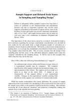
. Figure 5.1 shows a hypothetical set of calibration measurements, with a single A
i
for each C
i
, along with the regression line that best describes these data.

Figure 5.1 A Hypothetical Calibration Curve,
Units are Arbitrary
steqm-5.fm Page 111 Friday, August 8, 2003 8:16 AM
©2004 CRC Press LLC
Regression (see Chapter 4 for a discussion of regression) is the method that is
used to predict the estimated measured concentration from the known standard
concentration (because the standards were prepared to a known concentration). The
result is a prediction equation of the form:
M
i
= β
0
+ β
1
• C
i
+ ε
i
[5.1]
Here M
i
, is the predicted mean of the measured values (the A
i,j
’s) at known
concentration C
i
, β
0
the estimated concentration at C
i

= 0, β
1
is the slope coefficient
that predicts M
i
from C
i
, and ε
i
is the error associated with the prediction of M
i
.
Unfortunately, Equation [5.1] is not quite what we want for our chemical
analysis method because it allows us to predict a measurement from a known
standard concentration. When analyses are actually being performed, we wish to use
the observed measurement to predict the unknown true concentration. To do this, we
must rearrange Equation [5.1] to give:
[5.2]
In Equation [5.2] β
0
and β
1
are the same as those in [5.1], but C
i
is the unknown
concentration of the compound of interest, M
i
is the measurement from sample i, and
ε '
i

is the error associated with the “inverse” prediction of C
i
from M
i
. This procedure
is termed inverse prediction because the original regression model was fit to predict
M
i
from C
i
, but then is rearranged to predict C
i
from M
i
. Note also that the error
terms in [5.1] and [5.2] are different because inverse prediction has larger errors than
simple prediction of y from x in a regular regression model.
Detection Limits
The point of this discussion is that the reported concentration of any chemical in
environmental media is an estimate with some degree of uncertainty. In the
calibration process, chemists typically define some C
n
value that is not significantly
different from zero, and term this quantity the “method detection limit.” That is, if
we used the ε ' distribution from [5.2] to construct a confidence interval for C, C
n
would be the largest concentration whose 95% (or other interval width) confidence
interval includes zero. Values below the limit of detection are said to be censored
because we cannot measure the actual concentration and thus all values less than Cn
are reported as “less than LOD,” “nondetect,” or simply “ND.” While this seems a

rather simple concept the statistical process of defining exactly what the LOD is for
a given analytical procedure is not (Gibbons, 1995).
Quantification Limits
Note that as might be expected from [5.2] all estimated C
i
values, , have an
associated error distribution. That is:
[5.3]
C
i
M
i
β
0
–
β
1

ε ’
i
+=
c
ˆ
i
c
ˆ
i
κ
i
ε

i
+=
steqm-5.fm Page 112 Friday, August 8, 2003 8:16 AM
©2004 CRC Press LLC
where κ
i
is the true but unknown concentration and ε
i
is a random error component.
When is small, it can have a confidence interval that does not include zero (thus
it is not an “ND”) but is still quite wide compared to the concentration being
reported. For example, one might have a dioxin concentration reported as 500 ppb,
but with a 95% confidence interval of 200 to 1,250 ppb. This is quite imprecise and
would likely be reported as below the “limit of quantification” or “less than LOQ.”
However, the fact remains that a value reported as below the limit of quantification
still provides evidence that the substance of interest has been identified.
Moreover, if the measured concentrations are unbiased, it is true that the average
error is zero. That is:
[5.4]
Thus if we have many values below the LOQ it is true that:
[5.5]
and for large samples,
[5.6]
That is, even if all values are less than LOQ, the sum is still expected to equal
the sum of the unknown but true measurements and by extension, the mean of a
group of values below the LOQ, but above the DL, would be expected to equal the
true sample mean.
It is worthwhile to consider the LOQ in the context of the calibration process.
Sometimes an analytic method is calibrated across a rather narrow range of standard
concentrations. If one fits a statistical model to such data, the precision of

predictions can decline rapidly as one moves away from the range of the data used
to fit the model. In this case, one may have artificially high LOQs (and Detection
Limit or DLs as well) as a result of the calibration process itself. Moreover, if one
moves to concentrations above the range of calibration one can also have
unacceptably wide confidence intervals. This leads to the seeming paradox of values
that are too large to be acceptably precise. This general problem is an issue of
considerable discussion among statisticians engaged in the evaluation of chemical
concentration data (see for example: Gilliom and Helsel, 1986; Helsel and Gilliom,
1986; Helsel, 1990a 1990b).
The important point to take away from this discussion is that values less than
LOQ do contain information and, for most purposes, a good course of action is to
simply take the reported values as the actual values (which is our expectation given
unbiased measurements). The measurements are not as precise as we would like, but
are better than values reported as “<LOQ.”
Another point is that sometimes a high LOQ does not reflect any actual
limitation of the analytic method and is in fact due to calibration that was performed
c
ˆ
i
ε
i∑
0=
c
ˆ
i
∑
κ
i∑
ε
i∑

+=
c
ˆ
i
∑
κ
i∑
=
steqm-5.fm Page 113 Friday, August 8, 2003 8:16 AM
©2004 CRC Press LLC
over a limited range of standard concentrations. In this case it may be possible to
improve our understanding of the true precision of the method being used by doing
a new calibration study over a wider range of standard concentrations. This will not
make our existing <LOQ observations any more precise, but may give us a better
idea of how precise such measurements actually are. That is, if we originally had a
calibration data set at 200, 400, and 800 ppm and discovered that many field
measurements are less than LOQ at 50 ppm, we could ask the analytical chemist to
run a new set of calibration standards at say 10, 20, 40, and 80 ppm and see how well
the method actually works in the range of concentrations encountered in the
environment. If the new calibration exercise suggests that concentrations above
15 ppm are measured with adequate precision and are thus “quantified,” we should
have greater faith in the precision of our existing less than LOQ observations.
Censored Data
More often, one encounters data in the form of reports where the original raw
analytical results are not available and no further laboratory work is possible. Here
the data consist of the quantified data that are reported as actual concentrations, the
less than LOQ observations that are reported as less than LOQ, together with the
concentration defining the LOQ and values below the limit of detection, that are
reported as ND, together with concentration defining the limit of detection (LOD). It
is also common to have data reported as “not quantified” together with a

“quantification limit.” Such a limit may reflect the actual LOQ, but may also
represent the LOD, or some other cutoff value. In any case the general result is that
we have only some of the data quantified, while the rest are defined only by a cutoff
value(s). This situation is termed “left censoring” in statistics because observations
below the censoring point are on the left side of the distribution.
The first question that arises is: “How do we want to use the censored data set?”
If our interest is in estimating the mean and standard deviation of the data, and the
number of nonquantified observations (NDs and <LOQs) is low (say 10% of the
sample or less), the easiest approach is to simply assume that nondetects are worth
1/2 the detection limit (DL), and that <LOQ values (LVs) are defined as:
LV = DL + ½ (LOQ − DL) [5.7]
This convention makes the tacit assumption that the distribution of nondetects is
uniformly distributed between the detection limit and zero, and that <LOQ values
are uniformly distributed between the DL and the LOQ. After assigning values to all
nonquantified observations, we can simply calculate the mean and standard
deviation using the usual formulae. This approach is consistent with EPA guidance
regarding censored data (e.g., EPA, 1986).
The situation is even easier if we are satisfied with the median and interquartile
range as measures of central tendency and dispersion. The median is defined for any
data set where more than half of the observations are quantified, while the
interquartile range is defined for any data set where at least 75% of the observations
are quantified.
steqm-5.fm Page 114 Friday, August 8, 2003 8:16 AM
©2004 CRC Press LLC
Estimating the Mean and Standard DevIation Using Linear Regression
As shown in Chapter 2, observations from a normal distribution tend to fall on
a straight line when plotted against their expected normal scores. This is true even
if some of the data are below the limit of detection (see Example 5.1). If one
calculates a linear regression of the form:
C = A + B • Z-Score [5.8]

where C is the measured concentration, A and B are fitted constants, and Z-Score is
the expected normal score based on the rank order of the data, A is an estimate of
the mean, µ, and B is an estimate of the standard deviation, σ (Gilbert, 1987; Helsel,
1990).
Expected Normal Scores
The first problem in obtaining expected normal scores is to convert the ranks of
the data into cumulative percentiles. This is done as follows:
1. The largest value in a sample of N receives rank N, the second largest
receives rank N − 1, the third largest receives rank N − 2 and so on until all
measured values have received a rank. In the event that two or more values
are tied (in practice this should happen very rarely; if you have many tied
values you need to find out why), simply assign one rank K and one rank
K − 1. For example if the five largest values in a sample are unique, and
the next two are tied, assign one rank 6 and one rank 7.
2. Convert each assigned rank, r, to a cumulative percentile, P, using the
formula:
[5.9]
We note that other authors (e.g., Gilliom and Helsel, 1986) have used
different formulae such as P = r/(N + 1). We have found that using P values
calculated using [5.8] provide better approximations to tabled Expected
Normal Scores (Rohlf and Sokol, 1969) and thus will yield more accurate
regression estimates of µ and σ .
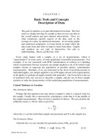
3. Once P values have been calculated for all observations, one can obtain
expected normal or Z scores using the relationship:
Z(P) = ϕ (P) [5.10]
Here Z(P) is the z-score associated with the cumulative probability P, and
ϕ is the standard normal inverse cumulative distribution function. This
function is shown graphically in Figure 5.2.
4. Once we have obtained Z values for each P, we are ready to perform a
regression analysis to obtain estimates of µ and σ .

P
r3/8
–()
N1/4
+()

=
steqm-5.fm Page 115 Friday, August 8, 2003 8:16 AM
©2004 CRC Press LLC
Example 5.1 contains a sample data set with 20 random numbers, sorted
smallest to largest, generated from a standard normal distribution (µ = 0 and σ = 1),
cumulative percentiles calculated from Equation 5.8, and expected normal scores
calculated from these P values. When we look at Example 5.1, we see that the
estimates for µ and σ look quite close to the usual estimates of µ and σ except for the
case where 75% of the data (15 observations) are censored. Note first that even
when we have complete data we do not reproduce the parametric values, µ = 0 and
σ = 1. This is because we started with a 20-observation random sample. For the case
of 75% censoring the estimated value for µ is quite a bit lower than the sample value
of − 0.3029 and the estimated value for σ is also a good bit higher than the sample
value of 1.0601. However, it is worthwhile to consider that if we did not use the
regression method for censored data, we would have to do something else. Let us
assume that our detection limit is really 0.32, and assign half of this value, 0.16, to
each of the 15 “nondetects” in this example and use the usual formulae to calculate
µ and σ . The resulting estimates are µ = 0.3692 and σ = 0.4582. That is, our
estimate for µ is much too large and our estimate for σ is much too small. The moral
here is that regression estimates may not do terribly well if a majority of the data is
censored, but other methods may do even worse.
The sample regression table in Example 5.1 shows where the Statistics
presented for the 4 models (20 observations, 15 observations, 10 observations,
5 observations) come from. The CONSTANT term is the intercept for the regression

equation and provides our estimate of µ, while the ZSCORE term is the slope of the
regression line and provides our estimate of σ . The ANOVA table is included
because the regression procedure in many statistical software packages provides this
as part of the output. Note that the information required to estimate µ and σ is found
Figure 5.2 The Inverse Normal Cumulative Distribution Function
steqm-5.fm Page 116 Friday, August 8, 2003 8:16 AM
©2004 CRC Press LLC
in the regression equation itself, not in the ANOVA table. The plot of the data with
the regression curve includes both the “detects” and the “nondetects.” However,
only the former were used to fit the curve. With real data we would have only the
detect values, but this plot is meant to show why regression on normal scores works
with censored data. That is, if the data are really log-normal, regression on those
data points that we can quantify will really describe all of the data. An important
point concerning using regression to estimate µ and σ is that all of the tools
discussed in our general treatment of regression apply. Thus we can see if factors
like influential observations or nonlinearity are affecting our regression model and
thus have a better idea of how good our estimates of µ and σ really are.
Maximum Likelihood
There is another way of estimating µ and σ from censored data that also does
relatively well when there is considerable left-censoring of the data. This is the
method of maximum likelihood. There are some similarities between this method
and the regression method just discussed. When using regression we use the ranks
of the detected observations to calculate cumulative percentiles and use the standard
normal distribution to calculate expected normal scores for the percentiles. We then
use the normal scores together with the observed data in a regression model that
provides us with estimates of µ and σ . In the maximum likelihood approach we start
by assuming a normal distribution for the log-transformed concentration. We then
make a guess as to the correct values for µ and σ . Once we have made this guess we
can calculate a likelihood for each observed data point, using the guess about µ and
σ and the known percentage, ψ , of the data that is censored. We write this result as

L(x
i
*µ, σ , ψ ). Once we have calculated an L for each uncensored observation, we
can calculate the overall likelihood of the data, L(X
*µ, σ , ψ ) as:
[5.11]
That is the overall likelihood of the data given µ, σ , and ψ , L(X
*µ, σ , ψ ), is the
product of the likelihoods of the individual data points. Such calculations are
usually carried out under logarithmic transformation. Thus most discussions are in
terms of log-likelihood, and the overall log-likelihood is the sum of the log-
likelihoods of the individual observations. Once L(X
*µ, σ , ψ ) is calculated there are
methods for generating another guess at the values for µ and σ , that yields an even
higher log-likelihood. This process continues until we reach values of µ and σ that
result in a maximum value for L(X
*µ, σ , ψ ). Those who want a technical discussion
of a representative approach to the likelihood maximization problem in the context
of censored data should consult Shumway et al. (1989).
The first point about this procedure is that it is complex compared to the
regression method just discussed, and is not easy to implement without special
software (e.g., Millard, 1997). The second point is that if there is only one censoring
value (e.g., detection limit) maximum likelihood and regression almost always give
LXµσψ,,()Lx
i
µσψ,,()
i1=
N
∏
=

steqm-5.fm Page 117 Friday, August 8, 2003 8:16 AM
©2004 CRC Press LLC
essentially identical estimates for µ and σ , and when the answers differ somewhat
there is no clear basis for preferring one method over the other. Thus for reasons of
simplicity we recommend the regression approach.
Multiply Censored Data
There is one situation where maximum likelihood methods offer a distinct
advantage over regression. In some situations we may have multiple “batches” of
data that all have values at which the data is censored. For example, we might have
a very large environmental survey where the samples were split among several labs
that had somewhat different instrumentation and thus different detection and
quantification limits. Alternatively, we might have samples with differing levels of
“interference” for the compound of interest by other compounds and thus differing
limits for detection and quantification. We might even have replicate analyses over
time with declining limits of detection caused by improved analytic techniques. The
cause does not really matter, but the result is always a set of measurements
consisting of several groups, each of which has its own censoring level.
One simple approach to this problem is to declare all values below the highest
censoring point (the largest value reported as not quantified across all groups) as
censored and then apply the regression methods discussed earlier. If this results in
minimal data loss (say, 5% to 10% of quantified observations), it is arguably the
correct course. However, in some cases, especially if one group has a high censoring
level, the loss of quantified data points may be much higher (we have seen situations
where this can exceed 50%). In such a case, one can use maximum likelihood
methods for multiply censored data such as those contained in Millard (1997) to
obtain estimates for µ and σ that utilize all of the available data. However, we
caution that estimation in the case of multiple censoring is a complex issue. For
example, the pattern of censoring can affect how one decides to deal with the data.
When dealing with such complex issues, we strongly recommend that a professional
statistician, one who is familiar with this problem area, be consulted.

Example 5.1
The Data for Regression
Y Data
(Random Normal)
Sorted Smallest to Largest
Cumulative Proportion
from Equation 5.8
Z-Scores from Cumulative
Proportions
− 2.012903
− 1.920049
− 1.878268
− 1.355415
− 0.986497
− 0.955287
− 0.854412
− 0.728491
− 0.508235
− 0.388784
0.030864
0.080247
0.129630
0.179012
0.228395
0.277778
0.327161
0.376543
0.425926
0.475307
− 1.868241

− 1.403411
− 1.128143
− 0.919135
− 0.744142
− 0.589455
− 0.447767
− 0.314572
− 0.186756
− 0.061931
steqm-5.fm Page 118 Friday, August 8, 2003 8:16 AM
©2004 CRC Press LLC
Statistics
• Summary Statistics for the Complete y Data, using the usual estimators:
Mean = − 0.3029 SD = 1.0601
• Summary Statistics for the Complete Data, using regression of the complete
data on Z- Scores:
Mean = − 0.3030 SD = 1.0902 R
2
= 0.982
• Summary Statistics for the 15 largest y observations (y = -0.955287 and
larger), using regression of the data on Z- Scores:
Mean = − 0.3088 SD = 1.1094 R
2
= 0.984
• Summary Statistics for the 10 largest y observations (y = − 0.168521 and
larger), using regression of the data on Z- Scores:
Mean = − 0.2641 SD = 1.0661 R
2
= 0.964
• Summary Statistics for the 5 largest y observations (y = 0.440684 and larger),

using regression of the data on Z- Scores:
Mean = − 0.5754. SD = 1.2966 R
2
= 0.961
The Regression Table and Plot for the 10 Largest Observations
− 0.168521
0.071745
0.084101
0.256237
0.301572
0.440684
0.652699
0.694994
1.352276
1.843618
0.524691
0.574074
0.623457
0.672840
0.722222
0.771605
0.820988
0.870370
0.919753
0.969136
0.061932
0.186756
0.314572
0.447768
0.589456

0.744143
0.919135
1.128143
1.403412
1.868242
Unweighted Least-Squares Linear Regression of Y
Predictor Variables Coefficient Std Error Student’s t P
Constant − 0.264 0.068 − 3.87 0.0048
Z-score 1.066 0.074 14.66 0.0000
The Data for Regression (Cont’d)
Y Data
(Random Normal)
Sorted Smallest to Largest
Cumulative Proportion
from Equation 5.8
Z-Scores from Cumulative
Proportions
steqm-5.fm Page 119 Friday, August 8, 2003 8:16 AM
©2004 CRC Press LLC
R-SQUARED 0.9641
Estimating the Arithmetic Mean and Upper Bounds on the Arithmetic Mean
In Chapter 2, we discussed how one can estimate the arithmetic mean
concentration of a compound in environmental media, and how one might calculate
an upper bound on this arithmetic mean. Our general recommendation was to use
the usual statistical estimator for the arithmetic mean and to use bootstrap
methodology (Chapter 6) to calculate an upper bound on this mean. The question at
hand is how do we develop estimates for the arithmetic mean, and upper bounds for
this mean, when the data are censored?
One approach that is appealing in its simplicity is to use the values of µ and σ ,
estimated by regression on expected normal scores, to assign values to the censored

observations. That is, if we have N observations, k of which are censored, we can
assume that there are no tied values and that the ranks of the censored observations
are 1 through k. We can then use these ranks to calculate P values using
Equation [5.9], and use the estimates P values to calculate expected normal scores
ANOVA Table
Source DF SS MS F P
Regression 1 3.34601 3.34601 214.85 0.0000
Residual 8 0.12459 0.01557
Total 9 3.47060
Figure 5.3 A Regression Plot of the Data Used in Example 5.1
steqm-5.fm Page 120 Friday, August 8, 2003 8:16 AM
©2004 CRC Press LLC
(Equation [5.10]). We then use the regression estimates of µ and σ to calculate
“values” for the censored observations and use an exponential transformation to
calculate observations in original units (usually ppm or ppb). Finally, we use the
“complete” data, which consists of estimated values for the censored observations
and observed values for the uncensored observations, together with the usual
formulae to calculate and s.
Consider Example 5.2. The estimates of µ and σ are essentially identical. What
is perhaps more surprising is the fact that the upper percentiles of the bootstrap
distribution shown Example 5.2 are also virtually identical for the complete and
partially estimated exponentially transformed data. Replacing the censored data
with their exponentially transformed expectations from the regression model and
then calculating and s using the resulting pseudo-complete data is a strategy that has
been recommended by other authors (Helsel, 1990b; Gilliom and Helsel, 1986;
Helsel and Gilliom, 1986). The use of the same data to estimate an upper bound for
is a relatively new idea, but one that flows logically from previous work. That is,
the use of the bootstrap technique to estimate an upper bound on is well established
for the case of uncensored data. As noted earlier (Chapter 2), environmental data is
almost always skewed to the right. That is, the distribution has a long “tail” that

points to the right. Except for cases of extreme censoring, this long tail always
consists of actual observations, and it is this long tail that plays the major role in
determining the bootstrap upper bound on . Our work suggests that the bootstrap is
a useful tool for determining an upper bound on whenever at least 50% of the data
are uncensored (Ginevan and Splitstone, 2002).
Example 5.2
Calculating the Arithmetic Mean and its Bootstrap Upper Bound
Y Data
(Random Normal)
Sorted Smallest to
Largest
Z-Scores from
Cumulative
Proportions
Data Calculated
from Estimates of
µ and σ
Exponential
Transform of
Calculated for
Censored and
Observed for
Uncensored
Censored
− 1.868240
− 1.403411
− 1.128143
− 0.919135
− 0.744142
− 0.589455

− 0.447767
− 0.314572
− 0.186756
− 0.061931
− 2.255831
− 1.760276
− 1.466813
− 1.243989
− 1.057429
− 0.892518
− 0.741464
− 0.599465
− 0.463200
− 0.330124
0.1047864
0.1719973
0.2306594
0.2882319
0.3473474
0.4096230
0.4764157
0.5491052
0.6292664
0.7188341
x
x
x
x
x
steqm-5.fm Page 121 Friday, August 8, 2003 8:16 AM

©2004 CRC Press LLC
Statistics
• Summary statistics for the complete exponentially transformed Y data from
Example 5.1 (column 1), using the usual estimators:
Mean = 1.2475 SD = 1.4881
• Summary statistics for the exponentially transformed Y data from column 4
above:
Mean = 1.2621 SD = 1.4797
• Bootstrap percentiles (2,000 replications) for the exponentially transformed
complete data from Example 5.1 and from column 4 of Example 5.2.
Zero Modified Data
The next topic we consider in our discussion of censored data is the case
referred to as zero modified data. In this case a certain percentage, Ζ %, of the data
are true zeros. That is, if we are interested in pesticide residues on raw agricultural
commodities, it may be that Ζ % of the crop was not treated with pesticide at all and
thus has zero residues. Similarly, if we are sampling groundwater for contamination,
− 0.168521
0.071745
0.084101
0.256237
0.301572
0.440684
0.652699
0.694994
1.352276
1.843618
0.061932
0.186756
0.314572
0.447768

0.589456
0.744143
0.919135
1.128143
1.403412
1.868242
Observed
0.8449135
1.0743813
1.0877387
1.2920589
1.3519825
1.5537696
1.9207179
2.0036971
3.8662150
6.3193604
50% 75% 90% 95%
Example 5.1 1.2283 1.4501 1.6673 1.8217
Example 5.2 1.2446 1.4757 1.7019 1.8399
Calculating the Arithmetic Mean and its Bootstrap Upper Bound (Cont’d)
Y Data
(Random Normal)
Sorted Smallest to
Largest
Z-Scores from
Cumulative
Proportions
Data Calculated
from Estimates of

µ and σ
Exponential
Transform of
Calculated for
Censored and
Observed for
Uncensored
steqm-5.fm Page 122 Friday, August 8, 2003 8:16 AM
©2004 CRC Press LLC
it may be that Ζ % of the samples represent uncontaminated wells and are thus true
zeros. In many cases, we have information on what Ζ % might be. That is, we might
know that approximately 40% of the crop was untreated or that 30% of the wells are
uncontaminated.
In such a case the expected proportion of samples with any residues θ (both
above and below the censoring limit(s)) is:
θ = 1 - (Ζ %/100) [5.12]
That is, if we have N samples, we would expect about L = N
• θ samples (L is
rounded to the nearest whole number) to have residues.
One simple, and reasonable, way to deal with true zeros is to assume a value for
Ζ %, calculate the number, L, of observations that we expect to have residues, and
then use L and O, the number of observations that have observed residues to
calculate regression estimates for µ and σ . That is, we assume that we have a sample
of size L, with O samples with observed residues. We then calculate percentiles and
expected normal scores assuming a sample of size L and proceed as in Example 5.1.
In this simple paradigm we could also estimate the L-zero values with undetected
residues using the approach shown in Example 5.2 by assigning regression estimated
values to these observations. We could then exponentially transform the values for
“contaminated” samples to get concentrations in original units, assign the value zero
to the N-L uncontaminated samples and use the usual estimator to calculate mean

contamination and the bootstrap to calculate an upper bound on the mean.
If we have a quite good idea of Ζ % and a fairly large sample (say, an L value of
30 or more with at least 15 samples with measured residues), this simple approach is
probably all we need, but in some cases we have an idea that Ζ % is not zero, but are
not really sure how large it is. Here one possibility is to use maximum likelihood
methods to estimate µ, σ, and Ζ %. Likewise we could also assume a distribution
reflecting our uncertainty about Ζ % (e.g., say we assume that Ζ % is uniformly
distributed between 10 and 50) and use Monte Carlo simulation methods to calculate
an uncertainty distribution for the mean. In practice, such approaches may be useful,
but both are beyond the scope of this discussion. We have again reached the point at
which a subject matter expert should be consulted.
Completely Censored Data
Sometimes we have a large number of observations with no detected
concentrations. Here it is common to assign a value of 1/2 the LOD to all
observations. This can cause problems because the purpose of risk assessment one
often calculates a hazard index (HI). The Hazard Index (HI) for N chemicals is
calculated as (EPA, 1986):
[5.13]HI
RfD
i
E
i

i1=
N
∑
1–
=
steqm-5.fm Page 123 Friday, August 8, 2003 8:16 AM
©2004 CRC Press LLC

where the RfD
i
is the reference dose, or level below which no adverse effect is
expected for the ith chemical compound, and E
i
is the exposure expected from that
chemical. A site with an HI of greater than one is assumed to present undue risks to
human health. If the number of chemicals is large and/or the LODs for the chemicals
are high, one can have a situation where the HI is above 1 for a site where no
hazardous chemicals have been detected!
The solution to this dilemma is to remember (Chapter 2) that if we have N
observations, we can calculate the median cumulative probability for the largest
sample observation, P(max), as:
[5.14]
For the specific case of a log-normal distribution, S
P
, the number of logarithmic
standard deviation error (σ ) units that are between the cumulative probability,
P(max) of the distribution, and the mean of the parent distribution, is found as the
Normal Inverse, Z
I
, of P(max), that is:
[5.15]
To get an estimate of the logarithmic mean, µ, of the log-normal distribution the
X
P
value, together with the LSE estimate and the natural logarithm of the LOD,
LN(LOD), are used:
[5.16]
The geometric mean, GM, is given by:

[5.17]
Note that quantity of interest for health risk calculations is often the arithmetic mean,
M, which can be calculated as:
[5.18]
(see Gilbert, 1987).
We can easily obtain P(max), but how can we estimate σ ? In general,
environmental contaminants are chemicals dissolved in a matrix (water, soil, peanut
butter). To the extent that the same forces operate to vary concentrations, the
variations tend to be multiplicative (e.g., if the volume of solvent doubles, the
concentrations of all solutes are halved). On a log scale this means that, in the same
matrix, high-concentration compounds should have an LSE that is similar to the LSE
Pmax() 0.5()
1N/
=
S
P
Z
I
Pmax()[]–
that standard normal deviate
corresponding to the cumulative
probability, P(max)





=
µ Ln LOD()S
P

σ–=
GM e
µ
=
Me
µ
σ
2
2

+


=
steqm-5.fm Page 124 Friday, August 8, 2003 8:16 AM
©2004 CRC Press LLC
of low-concentration compounds, because both have been subjected to a similar
series of multiplicative concentration changes. Thus we can estimate σ by assuming
it is similar to the observed σ values of other compounds with large numbers of
detected values. Of course, when deriving an LSE in this manner, one should restrict
consideration to chemically similar pairs of compounds (e.g., metal oxides;
polycyclic aromatic hydrocarbons). Nonetheless, the σ value of calcium in
groundwater might be a useful approximation for the σ of cadmium in groundwater.
This approach, together with defensibly conservative assumptions, could be used to
estimate a σ for almost any pollutant or food contaminant. Moreover, we need not
restrict ourselves to a single σ estimate; we could try a range of values to evaluate the
sensitivity of our estimate for M. The procedure discussed here is presented in more
detail in Ginevan (1993). An example calculation is shown in Example 5.3.
Note also that if one can calculate a lower bound for P(max). That is, if one wants
a 90% lower bound for P(max) one uses 0.10 instead of 0.50 in Equation [5.14];

similarly, if one wants a 95% lower bound one uses 0.05. More generally, if one
wants a 1 −α lower bound on P(max), one uses α instead of 0.5. This approach may
be useful because using a lower bound on P(max) will give an upper bound on µ,
which may be used to ensure a “conservative” (higher) estimate for the GM.
Example 5.3
Bounding the mean when all observations are below the LOD:
1. Assume we have a σ value of 1 (experience suggests that many environ-
mental contaminants have σ between 0.7 and 1.7) and a sample size, N, of
200. Also assume that the LOD is 1 part per billion (1 ppb).
2. To estimate a median value for the geometric mean we use the relationship:
Thus, P(max) = 0.99654.
3. We now determine from [5.15] that S
P
= Z
I
(0.99654) = 2.7007.
4. The estimate for the logarithmic mean, µ, is given by [5.16] and is:
5. Using [5.17] the estimate for the geometric mean, GM, is:
Pmax() 0.5
1200/
=
µ Ln LOD()S
P
σ•–=
µ Ln 1()– 2.7007 1•()–
µ 2.7007–=
GM e
µ
=
steqm-5.fm Page 125 Friday, August 8, 2003 8:16 AM

©2004 CRC Press LLC
6. We can also get an estimate for the arithmetic mean from [5.18] as:
Note that even the estimated arithmetic mean is almost 5-fold less than the default
estimate of 1/2 the LOD or 0.5.
When All Else Fails
Compliance testing presents yet another set of problems in dealing with
censored data. In many respects this is a simpler problem in that a numerical
estimate of average concentration is not necessarily required. However, this
problem is perhaps a much more common dilemma than the assessment of exposure
risk. Ultimately all one needs to do is demonstrate compliance with some standard
of performance within some statistical certainty.
The New Process Refining Company has just updated its facility in Gosh
Knows Where, Ohio. As a part of this facility upgrade, New Process has installed a
new Solid Waste Management Unit (SWMU), which will receive some still bottom
sludge. The monitoring of quality of groundwater around this unit is required under
their permit to operate.
Seven monitoring wells have been appropriately installed in the area of the
SWMU. Two of these wells are thought to be up gradient and the remaining five
down gradient of the SWMU. These wells have been sampled quarterly for the first
year after installation to establish site-specific “background” groundwater quality.
Among the principal analytes for which monitoring is required is Xylene. The
contract-specified MDL for the analyte is 10 microgram per liter (µg/L). All of the
analytical results for Xylene are reported as below the MDL. Thus, one is faced with
characterizing the background concentrations of Xylene in a statistically meaningful
way with all 28 observations reported as <10 µg/L.
One possibility is to estimate the true proportion of “background” Xylene
measurements that can be expected to be above the MDL. This proportion must be
somewhere within interval 0.0, and 1.0. Here 0.0 indicates that Xylene will NEVER
be observed above the MDL and 1.0 indicates that Xylene will ALWAYS be
observed above the MDL. The latter is obviously not correct based upon the existing

evidence. While the former is a possibility, it is unlikely that a Xylene concentration
will never be reported above the MDL with continued monitoring of background
water quality.
GM e
2.7007–
=
GM 0.06716=
Me
µ
σ
2
2

+


=
Me
2.7002– 12⁄+
=
M0.1107=
steqm-5.fm Page 126 Friday, August 8, 2003 8:16 AM
©2004 CRC Press LLC
There are several reasons why we should consider the likelihood of a future
background groundwater Xylene concentration reported above the MDL. Some of
these are related to random fluctuations in the analytical and sampling techniques
employed. A major reason for expecting a future detected Xylene concentration is
that the New Process Refining Company facility lies on top of a known petroleum-
bearing formation. Xylenes occur naturally in such formations (Waples, 1985).
Fiducial Limits

Thus, the true proportion of Xylene observations possibly above the MDL is not
well characterized by the point estimate, 0.0, derived from the available evidence.
This proportion is more logically something greater than 0.0, but certainly not 1.0.
We may bound this true proportion by answering the question: “What are possible
values of the true proportion, p, of Xylene observations greater than the MDL which
would likely have generated the available evidence?”
First, we need to define “likely” and then find a relationship between this
definition and p. We can define a “likely” interval for p as those values of p that
could have generated the current evidence with 95 percent confidence (i.e., a
probability of 0.95). Since there are only two alternatives, either a concentration
value is above, or it is below, the MDL, the binomial density model introduced in
Equation [2.23] provides a useful link between p and the degree of confidence.
The lowest possible value of p is 0.0. As discussed in the preceding paragraphs,
if the probability of observing a value greater than the MDL is 0.0, then the sample
results would occur with certainty. The upper bound, p
u
, of our set of possible values
for p will be the value that will produce the evidence with a probability of 0.05. In
other words we are 95 percent confident that p is less than this value. Using
Equation [2.23], this is formalized as follows:
Solving for p
u
,[5.13]
The interval 0.0 ≤ p ≤ 0.10 not only contains the “true” value of p with 95 percent
confidence, it is also a “fiducial interval.” Wang (2000) provides a nice discussion of
fiducial intervals including something of their history. Fiducial intervals for the
binomial parameter p were proposed by Clopper and Pearson in 1934.
The construction of a fiducial interval for the probability of getting an observed
concentration greater than the MDL is rather easy when all of the available
observations are below the MDL. However, suppose one of our 28 “background”

groundwater quality observations is above the MDL. Obviously, this eliminates 0.0
as a possible value for the lower bound.
We may still find a fiducial interval, p
L
≤ p ≤ p
U
, by finding the bounding values
that satisfy the following relations:
fx=0()
28
0



P
u
0
1p
u
–()
28
= 0.05≥
p
u
1.0 0.05()
128/
– 0.10==
steqm-5.fm Page 127 Friday, August 8, 2003 8:16 AM
©2004 CRC Press LLC
[5.14]

Here (1 −α ) designates the desired degree of confidence, X represents the observed
number of values exceeding the MDL. Slightly rewriting [5.14] as follows, we may
use the identity connecting the beta distribution and the binomial distribution to
obtain values for p
L
and p
U
(see Guttman, 1970):
[5.15]
In the hypothetical case of one out of 28 observations reported as above the MDL,
p
L
= 0.0087 and p
U
= 0.1835. Therefore the 95 percent fiducial, or confidence,
interval (0.0087, 0.1835) for p.
The Next Monitoring Event
Returning to the example provided by New Process Refining Company, we
have now bounded the probability that a Xylene concentration above the MDL will
be observed. The fiducial interval for this probability based upon the background
monitoring event is (0.0, 0.10). One now needs to address the question of when there
should be concern that groundwater quality has drifted from background. If on the
next monitoring event composed of a single sample from each of the seven wells,
one Xylene concentration was reported as above the MDL would that be cause for
concern? What about two above the MDL? Or perhaps three?
Christman (1991) presents a simple statistical test procedure to determine whether
or not one needs to be concerned about observations greater than the MDL. This
procedure determines the minimum number of currently observed monitoring results
reported as above the MDL that will result in concluding there is a potential problem,
while controlling the magnitude of the Type I and Type II decision errors.

The minimum number of currently observed monitoring results reported as
above the MDL will be referred to as the “critical count” for brevity. We will
represent the critical count by “K.” The Type I error is simply the probability of
observing K or more monitoring results above the MDL on the next round of
groundwater monitoring given the true value of p is within the fiducial interval:
[5.16]
where
Prob x X p
L
<()α2⁄=
Prob x X p
U
>()α2⁄=
Prob x X p
L
<()α2⁄=
Prob x X p
U
≤()α2⁄=
Prob Type I Error K()1.0
7
k



p
k
1.0 p–()
7k–
k0=

K1–
∑
–=
0.0p0.1≤≤()
steqm-5.fm Page 128 Friday, August 8, 2003 8:16 AM
©2004 CRC Press LLC
This relationship is illustrated in Figure 5.4.
If one were to decide that a possible groundwater problem exists based upon one
exceedance of the MDL in the next monitoring event, i.e., a critical count of 1, the
risk of falsely reaching such a conclusion dramatically increases to nearly 50 percent
as the true value of p approaches 0.10, the upper limit of the fiducial interval. If we
choose a critical count of 3, the risk of falsely concluding a problem exists remains
at less than 0.05 (5 percent).
Fixing the Type I error is only part of the equation in choosing an appropriate
critical count. Consistent with Steps 5, 6, and 7 of the Data Quality Objects Process
(USEPA, 1994), one needs to consider the risk of falsely concluding that no
groundwater problem exists when in fact p has exceeded the upper fiducial limit.
This is the risk of making a decision error of Type II. The probability of a Type II
error is easily determined via Equation [5.17]:
[5.17]
where
Figure 5.4 Probability of Type I Error
for Various Critical Counts
Prob Type II Error K()1.0
7
k



p

k
1.0 p–()
7k–
k0=
K1–
∑
–=
0.1 p<()
steqm-5.fm Page 129 Friday, August 8, 2003 8:16 AM
©2004 CRC Press LLC
Note that the risk of making a Type II error is near 90 percent for a critical count
of 3, Prob(Type II Error|K = 3) >
0.90, when p is near 0.10 and remains greater than
20 percent for values of p near 0.5. Therefore, while a critical count of 3 minimizes
the operator’s risk of a falsely concluding a problem may exist (Type I error) the risk
of falsely concluding no problem exists (Type II error) remains quite large.
Suppose that a critical count of two seems reasonable, what are the implications
for the groundwater quality decision making? New Process Refining Company must
be willing to run a greater than 5 percent chance of a false allegation of groundwater
quality degradation if the true p is between 0.05 and 0.10. Conversely, the other
stakeholders must take a greater than 20 percent chance that no degradation of
quality will be found when the true p is between 0.10 and 0.37. This interval of
0.05 ≤ p ≤ 0.37 is often referred to as the “gray of region” (USEPA, 1994, pp. 34–36).
This is a time for compromise and negotiation.
Epilogue
There is no universal tool to use in dealing with censored data. The tool one chooses
to use depends upon the decision one is attempting to make and the consequences
associated with making an incorrect decision. Even then there may be several tools that
Figure 5.5 Probability of Type II Errors
for Various Critical Counts

steqm-5.fm Page 130 Friday, August 8, 2003 8:16 AM
©2004 CRC Press LLC
can accomplish the same task. The choice among them depends largely on the
assumptions one is willing to make. As with all statistical tools, the choice of the best
tool for the job depends upon the appropriateness of the underlying assumptions and the
recognition and balancing of the risks of making an incorrect decision.
steqm-5.fm Page 131 Friday, August 8, 2003 8:16 AM
©2004 CRC Press LLC
References
Christman, J. D., 1991, “Monitoring Groundwater Below Limits of Detection,”
Pollution Engineering, January.
Clopper, C. J. and Pearson, E. S., 1934, “The Use of Confidence or Fiducial Limits
Illustrated in the Case of the Binomial,” Biometrika, 26, 404–413.
Environmental Protection Agency (EPA), 1986, Guidelines for the Health Risk
Assessment of Chemical Mixtures, 51 FR 34014-34025.
Gibbons, R. D., 1995, “Some Statistical and Conceptual Issues in the Detection of
Low Level Environmental Pollutants,” Environmental and Ecological Statistics
2: 125–144.
Gilbert, R. O., 1987, Statistical Methods for Environmental Pollution Monitoring,
Van Nostrand Reinhold, New York.
Gilliom, R. J. and Helsel, D. R., 1986, “Estimation of Distributional Parameters for
Censored Trace Level Water Quality Data 1: Estimation Techniques,” Water
Resources Research, 22: 135–146.
Ginevan, M. E., 1993, “Bounding the Mean Concentration for Environmental
Contaminants When all Observations are below the Limit of Detection,”
American Statistical Association, 1993, Proceedings of the Section on Statistics
and the Environment, pp. 123–128.
Ginevan, M. E. and Splitstone, D. E., 2001, “Bootstrap Upper Bounds for the
Arithmetic Mean of Right-Skewed Data, and the Use of Censored Data,”
Environmetrics (in press).

Guttman, I., 1970, Statistical Tolerance Regions: Classical and Bayesian, Hafner
Publishing Co., Darien, CT.
Helsel, D. R. and Gilliom, R. J., 1986, “Estimation of Distributional Parameters for
Censored Trace Level Water Quality Data 2: Verification and Applications,”
Water Resources Research, 22: 147–155.
Helsel, D. R., 1990a, “Statistical Analysis of Data Below the Detection Limit: What
Have We Learned?, Environmental Monitoring, Restoration, and Assessment:
What Have We Learned?”, Twenty-Eighth Hanford Symposium on Health and
the Environment, October 16–19, 1989, ed. R.H. Gray, Battelle Press,
Columbus, OH.
Helsel, D. R., 1990b, “Less Than Obvious: Statistical Treatment of Data below the
Detection Limit,” Environmental Science and Technology, 24: 1766–1774.
Millard, S. P., 1997, Environmental Stats for S-Plus. Probability, Statistics and
Information, Seattle, WA.
Rohlf, F. J. and Sokol, R. R., 1969, Statistical Tables, Table AA, W. H. Freeman,
San Francisco.
Shumway, R. H., Azari, A. S., and Johnson, P., 1989, “Estimating Mean
Concentrations Under Transformation for Environmental Data with Detection
Limits,” Technometrics, 31: 347–356.
USEPA, 1994, Guidance for the Data Quality Objectives Process, EPA QA/G-4.
steqm-5.fm Page 132 Friday, August 8, 2003 8:16 AM
©2004 CRC Press LLC
Wang, Y. H., 2000, “Fiducial Intervals: What Are They?,” The American
Statistician, 52(2): 105–111.
Waples, D. W., 1985, Geochemistry in Petroleum Exploration, Reidl Publishing,
Holland.
steqm-5.fm Page 133 Friday, August 8, 2003 8:16 AM
©2004 CRC Press LLC