báo cáo khoa học: " Transcript and metabolite analysis in Trincadeira cultivar reveals novel information regarding the dynamics of grape ripening" potx
Bạn đang xem bản rút gọn của tài liệu. Xem và tải ngay bản đầy đủ của tài liệu tại đây (3.35 MB, 9 trang )
METH O D O LOG Y AR T I C LE Open Access
Multiallelic epistatic model for an out-bred cross
and mapping algorithm of interactive
quantitative trait loci
Chunfa Tong
1,2
, Bo Zhang
1
, Zhong Wang
2,3
, Meng Xu
1
, Xiaoming Pang
3
, Jingna Si
3
, Minren Huang
1
and
Rongling Wu
3,2*
Abstract
Background: Genetic mapping has proven to be powerful for studying the genetic architecture of complex traits
by characterizing a network of the underlying interacting quantitative trait loci (QTLs). Current statistical models for
genetic mapping were mostly founded on the biallelic epistasis of QTLs, incapable of analyzing multiallelic QTLs
and their interactions that are widespread in an outcrossing population.
Results: Here we have formulated a general framework to model and define the epistasis between multiallelic
QTLs. Based on this framework, we have derived a statistical algorithm for the estimation and test of multiallelic
epistasis between different QTLs in a full-sib family of outcrossing species. We used this algorithm to genomewide
scan for the distribution of mul-tiallelic epistasis for a rooting ability trait in an outbred cross derived from two
heterozygous poplar trees. The results from simulation studies indicate that the positions and effects of multiallelic
QTLs can well be estimated with a modest sample and heritability.
Conclusions: The model and algorithm developed provide a useful tool for better characterizing the genetic
control of complex traits in a heterozy gous family derived from outcrossing species, such as forest trees, and thus
fill a gap that occurs in genetic mapping of this group of important but underrepresented species.
Background
Approaches for quantitative trait locus (QTL) mapping
were developed originally for experimental crosses, such
as the backcross, double haploid, RILs or F
2
, derived
from inbred lines [1-3]. Because of the homoz ygosity of
inbred lines, the Mendelian (co)segregation of all mar-
kers each with two alternative alleles in such crosses can
be observed directly. In practice, there is also a group of
species of great economical and environmental impor-
tance - out-crossing species, such as forest trees, in
which traditional QTL mapping approaches cannot be
appropriately used. For these species, it is difficult or
impossible to generate inbred lines due to long genera-
tion intervals and high heterozygosity [4], although
experimental hybrids have been commercially used in
practical breeding programs.
For a given outbred line, some markers may be het-
erozy gous, whereas others may be homozygous over the
genome. All markers may, or may not, have t he same
allele system between any two outbred lines used for a
cross. Also, for a pair of heterozygous loci, their allelic
configuration along two homologous chromosomes (i.e.,
linkage phase) cannot be observed from the segregation
pattern of genotypes in the cross [5,6]. Unfortunately, a
consistent number of alleles across different markers
and their known linkage phases are the prerequisites fo r
statistical mapping approaches described for the back-
cross or F
2
. Grattap aglia and Sederoff [7] proposed a so-
called pseudo-test backcross strategy for linkage map-
ping in a controlled cross between two outbred parents.
This strategy is powerful for the linkage analysis of
those testcross markers that are heterozygous in one
parent and null in the other, although it fails to consider
many other marker cross types, such as intercross
* Correspondence:
3
Center for Computational Biology, National Engineering Laboratory for Tree
Breeding, Key Laboratory of Genetics and Breeding in Forest Trees and
Ornamental Plants, Beijing Forestry University, Beijing 100083, China
Full list of author information is available at the end of the article
Tong et al. BMC Plant Biology 2011, 11:148
/>© 2011 Tong et al; licensee BioMed Central Ltd. This is an Open Access article distributed under the terms of the Creative Common s
Attribution License (http://creativecomm ons.org/licenses/by/2.0), which permits unrestricted use, distribution, and reproductio n in
any medium, provided the original work is prop erly cited.
markers and dominant markers, that occur f or an
outbred cross. Maliepaard et al. [8] derived numerous
formulas for estimating the linkage between different
types of m arkers by co rrectly determining the linkage
phase of markers. A general model has been d eveloped
for simultaneous estimation of the linkage and linkage
phase for any marker cross type in outcrossing popula-
tions [9,10]. Stam [11] wrote powerful software for inte-
grating genetic linkage maps using different types of
markers.
Statistical methods for QTL mapping in a full-sib
family of outcrossing species have not receive d adequate
attention. Lin et al. [12] developed a model that takes
into account uncertainties about the number of alleles
across the genome. Wu et al. [13] used this model to
reanalyze a full-sib family data for poplar trees [14],
leading to the detection of new QTLs for biomass traits
which were not discovered by traditional approaches.
With increasing recognition of the role of epistasis in
controlling and maintaining quantitative variation [15],
it is crucial to extend Lin et al.’smodeltomaptheepi-
static of QTLs by which to elucidate a detailed and
comprehensive perspective on the genetic architecture
of a quantitative trait. However, the well-established the-
ory and model for epistasis are mostly based o n biallelic
genes [ 16] and their estima tion and test are made for a
pedigree derived from inbred lines [17]. Until now, no
models and algorithms have been available for charac-
terizing the epistasis of multiallelic QTLs in an outcross-
ing population.
In this article, we will extend the theory for biallelic
epistasis to model the epistasis between different QTLs
each with multiple alleles. The multiallelic epistatic the-
ory is then implemented into a statistical model for
QTL mapping based on a mixturemodel.Wehave
derived a closed form for the estimation of the main
and interactive e ffects of multialle lic QTLs within the
EM framework. Our model allows geneticists to test the
effects of individual genetic components on trait varia-
tion. The estimating model has been investigated
through simulation studies and validated by an example
of QTL mapping for poplar trees [18]. The algorithm
has b een packed t o a newly developed package of soft-
ware, 3FunMap, derived to map QTLs in a full-sib
family [19].
Quantitative Genetic Model
Additive-dominance Model
Randomly select two heterozygous lines as parents P
1
and P
2
to produce a full-sib family, in which a QTL will
form four genotypes if the two lines have complet ely dif-
ferent allele systems. Let μ
uv
be the value of a QTL geno-
type inheriting allele u (u=1,2) from parent P
1
and allele
v (v =3,4)fromparentP
2
. Based on quan titative genetic
theory, this genotypic value can be partitioned into the
additive and dominant effects as follows:
μ
uv
= μ + α
u
+ β
v
+
γ
uv
,
(1)
where μ is the overall mean, a
u
and b
v
are the allelic
(additive) effects of allele u and v, respectively, and g
uv
is
the interaction (dominant) effect at the QTL. Consider-
ing all possible alleles and allele combinations between
the t wo parent, there are a total of four additive effects
( a
1
and a
2
from parent P
1
and b
3
and b
4
from parent
P
2
and four dominant effects (g
13
, g
14
, g
23
and g
34
). But
these additive and dominant effects are not inde pendent
and, therefore, are not estimable. After parameterization,
there are two independent additive effects, a = a
1
=-a
2
and b
3
= b
3
=-b
4
, and one dominant effect, g = g
13
=
-g
14
=-g
23
= g
24
, to be estimated.
Let u =(μ
uv
)
4×1
and a =(μ, a, b, g)
T
, which can be
connected by a design matrix D. We have
u
= Da
,
where
D =
⎡
⎢
⎢
⎣
1111
11−1 −1
1 −11−1
1 −1 −11
⎤
⎥
⎥
⎦
.
The expression of a can be ob tai ned from the expres-
sion of u by
a
= D
−
1
u.
(2)
Additive-dominance-epistatic Model
If there are two segregating QTL in the full-sib family,
the epistatic effects due to their n onallelic interactions
should be considered. The theory for epistasis in an
inbred family [16] can be readily extended to specify dif-
ferent epistatic components for outbred crosses. Con-
sider two epistatic multiallelic QTL, each of which has
four different genotypes, 13, 14, 23, and 24, in the
outbred progeny. Let
μ
u
1
v
1
/
u
2
v
2
be the genotypic value
for QTL genotype u
1
v
1
/u
2
v
2
for u
1
,u
2
=1,2andv
1
,v
2
=
3,4 and
u
=(μ
u
1
v
1
/
u
2
v
2
)
be the corresponding mean vec-
tor. The two-QTL genotypic value is partitioned into
different components as follows:
μ
u
1
v
1
/u
2
v
2
= μ + α
1
+ β
1
+ γ
1
+ α
2
+ β
2
+ γ
2
+ I
αα
+ I
α
β
+ I
β
α
+ I
ββ
+ J
α
γ
+ J
βγ
+ K
γ
α
+ K
γβ
+ L
γγ
(3)
where
(1) μ is the overall mean;
Tong et al. BMC Plant Biology 2011, 11:148
/>Page 2 of 9
(2) a
1
is the additive effect due to the substitution
from allele 1 to 2 at the first QTL;
(3) b
1
is the additive effect due to the substitution
from allele 3 to 4 at the first QTL;
(4) g
1
is the dominant effect due to the interaction
between alleles from different parents;
(5) a
2
is the additive effect due to the substitution
from allele 1 to 2 at the second QTL;
(6) b
2
is the additive effect due to the substitution
from allele 3 to 4 at the second QTL;
(7) g
2
is the dominant effect due to the interaction
between alleles from different parents;
(8) I
aa
is the additive × additive epistatic effect due
to the interaction between the substitutions from
allele 1 to 2 at the first and second QTLs;
(9) I
ab
is the additive × additive epistat ic effect due
to the interaction between the substitutions from
allele 1 to 2 at the first QTL and from allele 3 to 4
at the second QTL;
(10) I
ba
is the additive × additive epistat ic effect due
to the interaction between the sub-stitutio ns from
allele 3 to 4 at the first QTL and from allele 1 to 2
at the second QTL;
(11) I
ab
is the additive × additive epistat ic effect due
to the interaction between the sub-stitutio ns from
allele 3 to 4 at the first and second QTLs;
(12) J
ag
is the additive × dominant epistatic effect
due to the interaction between the substitutions
from allele 1 to 2 at the first QTL and the dominant
effect at the second QTL;
(13) J
bg
is the additive × dominant epistatic effect
due to the interaction between the substitutions
from allele 3 to 4 at the first QTL and the dominant
effect at the second QTL;
(14) K
ga
is the dominant × additive epistatic effect
due to the interaction between the domin ant effect
atthefirstQTLandthesubstitutions from allele 1
to 2 at the second QTL;
(15) K
gb
is the dominant × additive epistatic effect
due to the interaction between the domin ant effect
atthefirstQTLandthesubstitutions from allele 3
to 4 at the second QTL;
(16) L
gg
is the dominant × dominant epistatic effect
due to the interaction between the dominant effects
at the first and second QTLs.
Genetic effect parameters for two interacting QTL are
arrayed in a =(μ, a
1
, b
1
, g
1
, a
2
, b
2
, g
2
, I
aa
, I
ab
, I
ba
, I
bb
,
J
ag
, J
bg
, K
ga
, K
gb
, L
gg
)
T
.Werelatethegenotypicvalue
vector and genetic effect vector by
u = Da
,
where design matrix
D =
⎡
⎢
⎢
⎢
⎢
⎢
⎢
⎢
⎢
⎢
⎢
⎢
⎢
⎢
⎢
⎢
⎢
⎢
⎢
⎢
⎢
⎢
⎢
⎢
⎢
⎢
⎢
⎣
1111111111111111
11111−1 −11−11−1 −1 −11−1 −1
1111−11−1 −11−11−1 −1 −11−1
1111−1 −11−1 −1 −1 −111−1 −11
11−1 −111111−1 −11−1 −1 −1 −1
11−1 −11−1 −11−1 −11−11−111
11−1 −1 −11−1 −111−1 −111−11
11−1 −1 −1 −11−1 −111
1−111−1
1 −11−1111−1 −111−11−1 −1 −1
1 −11−11−1 −1 −111−11−1 −111
1 −11−1 −11−11−1 −111−11−11
1 −11−1 −1 −1111−1 −1 −1111−1
1 −1 −11111−1 −1 −1 −1 −1 −11
11
1 −1 −111−1 −1 −11−11111−1 −1
1 −1 −11−11−11−11−111−11−1
1 −1 −11−1 −111111−1 −1 −1 −11
⎤
⎥
⎥
⎥
⎥
⎥
⎥
⎥
⎥
⎥
⎥
⎥
⎥
⎥
⎥
⎥
⎥
⎥
⎥
⎥
⎥
⎥
⎥
⎥
⎥
⎥
⎥
⎦
.
Thus, the ge netic effect vector can be expressed, in
terms of the genotypic value vector, as
a
= D
−1
1
u.
(4)
Ifwehavealleles1=3and2=4foranoutbred
family, Equations 1 and 3 will be reduced to traditional
biallelic additive-do minant and biallelic additive-domi-
nant-epistatic genetic models, respectively [20].
Statistical Model
Likelihood
Suppose there is a full-sib family of size n derived from
two outbred lines. Consider two interacting QTLs for a
quantitative trait. Let u
1
v
1
and u
2
v
2
denote a general
genotype at QTL 1 and 2, respectively, wher e u
1
and u
2
(u
1
,u
2
= 1,2) are the alleles inherited from parent P
1
and
v
1
and v
2
(v
1
,v
2
= 3,4) are the alleles inherited from par-
ent P
2
. The linear model of the trait value (y
i
) for indivi-
dual i affected by the two QTLs is written as
y
i
=
2
u
1
=1
4
v
1
=3
2
u
2
=1
4
v
2
=3
ξ
iu
1
v
1
/u
2
v
2
μ
u
1
v
1
/u
2
v
2
+ ei
,
(5)
where
ξ
iu
1
v
1
/
u
2
v
2
is the indicator variable for QTL geno-
types defined as 1 if a particular genotype u
1
v
1
/u
2
v
2
is
considered for individual i and 0 otherwise, and e
i
is th e
residual error normally distributed with mean 0 and var-
iance s
2
. The probability with which individual i car ries
QTL genotype u
1
v
1
/u
2
v
2
can be inferred from its marker
genotype, with this conditional probability expressed as
ω
u
1
v
1
/
u
2
v
2
|
i
[20].
The log-likelihood of the putative QTLs given the trait
value (y) and marker information (M) is given by
L(|y, M)=
n
i=1
2
u
1
=1
4
v
1
=3
2
u
2
=1
4
v
2
=3
ω
u
1
v
1
/u
2
v
2
|i
f
u
1
v
1
/u
2
v
2
(y
i
)
,
(6)
Tong et al. BMC Plant Biology 2011, 11:148
/>Page 3 of 9
where Θ is the v ector for unknown parameters that
include the QTL position expressed by the conditional
probabilities
ω
u
1
v
1
/u
2
v
2
|i
,QTLgenotypicvalues
μ
u
1
v
1
/u
2
v
2
and the residual variance (s
2
). The first para-
meters, denoted by Θ
p
, are contained in the mixture
proportions of the above model, whereas the second
two, denoted by Θ
q
, are quantitative genetic parameters.
Normal distribution density
fu
1
v
1
/u
2
v
2
(
y
i
)
has mean
μ
u
1
v
1
/
u
2
v
2
and variance s
2
.
EM Algorithm
The standard EM algorithm is developed to obtain the
estimates of the unknown vector. By differentiating the
log-likelihood of equation (6) with respect to two groups
of unknown parameters (Θ
p
, Θ
q
), we have
∂
∂
log L(|y, M)
=
n
i=1
2
u
1
=1
4
v
1
=3
2
u
2
=1
4
v
2
=3
f
u
1
v
1
/u
2
v
2
(yi)
∂
∂
p
ω
u
1
v
1
/u
2
v
2
|i
+ ω
u
1
v
1
/u
2
v
2
|i
∂
∂
q
f
u
1
v
1
u
2
v
2
(yi)
2
u
1
=1
4
v
1
=3
2
u
2
=1
4
v
2
=3
ωu
1
v
1
/u
2
v
2
|ifu
1
v
1
/u
2
v
2
(y
i
)
=
n
i=1
2
u
1
=1
4
v
1
=3
2
u
2
=1
4
v2=3
⎡
⎢
⎢
⎣
ωu
1
v
1
/u
2
v
2
|if u
1
v
1
/u
2
v
2
(yi)
1
ωu
1
v
1
/u
2
v
2
|i
∂
∂
p
ω
uv
|i
2
u
1
=1
4
v
1
=3
2
u
2
=1
4
v
2
=3
ω
u
1
v
1
/u
2
v
2
|i
f
u
1
v
1
/u
2
v
2
(yi)
+
ω
u
1
v
1
/u
2
v
2
|i
f
u
1
v
1
/u
2
v
2
(yi)
∂
∂
q
log f
u
1
v
1
/u
2
v
2
(yi)
2
u
1
=1
4
v
1
=3
2
u
2
=1
4
v
2
=3
ω
u
1
v
1
/u
2
v
2
|i
f
u
1
v
1/
u
2
v
2
(y
i
)
⎤
⎥
⎥
⎦
=
n
i=1
2
u
1
=1
4
v
1
=3
2
u
2
=1
4
v
2
=3
u
1
v
1
/u
2
v
2
|i
1
ω
u
1
v
1
/u
2
v
2
|i
∂
∂
p
ω
u
1
v
1
/u
2
v
2
|i
+
∂
∂
q
log f
u
1
v
1
/u
2
v
2
(y
i
)
,
where we define
u
1
v
1
/u
2
v
2
|i
=
ω
u
1
v
1
/u
2
v
2
|i
f
u
1
v
1
/u
2
v
2
(yi)
2
u
1
=1
4
v
1
=3
2
u
2
=1
4
v
2
=3
ω
u
1
v
1
/u
2
v
2
|i
f
u
1
v
1
/
u
2
v
2
(y
i
)
(7)
which could be thought of as a posterior probabilit y
that individual i has a QTL genotype u
1
v
1
/u
2
v
2
.
In the E step, calculate the posterior probabilities of
QTL genotypes given the marker genotype of individual
i by equation (7). In the M step, estimate the maximum
likel ihood estimates (MLEs) of the unknown parameters
by solving
∂
∂
log L( |y, M)=0
.
. The closed forms for
estimating the genotypic values and residual variance
are derived as
ˆμ
u
1
v
1
/u
2
v
2
=
2
u
1
=1
4
v
1
=3
2
u
2
=1
4
v
2
=3
u
1
v
1
/u
2
v
2
|i
y
i
2
u
1
=1
4
v
1
=3
2
u
2
=1
4
v
2
=3
u
1
v
1
/u
2
v
2
|i
ˆσ
2
=
1
n
n
i=1
2
u
1
=1
4
v
1
=3
2
u
2
=1
4
v
2
=3
y
i
ˆμ
u
1
v
1
/u
2
v
2
2
u
1
v
1
/u
2
v
2
|i
·
(8)
By giving initial values for the parameters, the E and
M steps are iterated until the estimates are stable. The
stable values are the M LEs of the unknown parameters.
Note that the QTL position within a marker interval
can be estimated by treating the position is fixed . Using
a grid search, we can obtain the MLE of t he QTL posi-
tion from the peak of the profile of the log-likelihood
ratio test statistics across a chromosome.
Hypothesis Tests
After the parameters are estimated, a number of hypoth-
esis tests can be made. The existence of a QTL can be
tested by formulating the null hypothesis expressed as
H
0
: μ
u
1
v
1
/u
2
v
2
≡ μ,foru
1
, v
1
=1,2andu
2
, v
2
=3,4
H
1
: at least one of the e
q
ualities above does not hold
.
(9)
The likelihoods under the reduced (H
0
) and full model
(H
1
) are calculated and their log-likelihood ratio (LR) is
then estimated by
LR = −2In
L
0
(
˜
p
,
˜
q
|y)
L
0
(
ˆ
p
,
ˆ
q
|y, M)
,
(10)
where the tilde s and hats are the MLEs under the H
0
and H
1
, respectively. The critical threshold for declaring
the existence of a QTL can be empirically determined
from permutation tests [21].
Hypothesis tests for different genetic effects including
the add itive (a
1
, b
1
, a
2
, b
2
), dominant (g
1
, g
2
) and addi-
tive × a dditive (I
aa
, I
ab
, I
ba
, I
bb
), additive × dominant
(J
ag
, J
bg
), dominant × additive (K
ga
, K
gb
) and dominant ×
dominant (L
gg
) epistatic effects can be formulated, with
the respective null hypotheses:
Under each null hypothesis, the genotypic values
should be constrained by
μ
13/13
+ μ
13/14
+ μ
13/23
+ μ
13/24
+ μ
14/13
+ μ
14/14
+ μ
14/23
+ μ
14/2
4
= μ
23
/
13
+ μ
23
/
14
+ μ
23
/
23
+ μ
23
/
24
+ μ
24
/
13
+ μ
24
/
14
+ μ
24
/
23
+ μ
24
/
2
4
(11)
for H
0
: a
1
=0,
μ
13/13
+ μ
13/14
+ μ
13/23
+ μ
13/24
+ μ
23/13
+ μ
23/14
+ μ
23/23
+ μ
23/2
4
= μ
14
/
13
+ μ
14
/
14
+ μ
14
/
23
+ μ
14
/
24
+ μ
24
/
13
+ μ
24
/
14
+ μ
24
/
23
+ μ
24
/
2
4
(12)
for H
0
: b
1
=0,
μ
13/13
+
μ
13/14
+
μ
14/13
+
μ
14/14
+
μ
23/13
+
μ
23/14
+
μ
24/13
+
μ
24/1
4
= μ
13
/
23
+ μ
13
/
24
+ μ
14
/
23
+ μ
14
/
24
+ μ
23
/
23
+ μ
23
/
24
+ μ
24
/
23
+ μ
24
/
2
4
(13)
for H
0
: a
2
=0,
μ
13/13
+
μ
13/23
+
μ
14/13
+
μ
14/23
+
μ
23/13
+
μ
23/23
+
μ
24/13
+
μ
24/23
= μ
13
/
14
+ μ
13
/
24
+ μ
14
/
14
+ μ
14
/
24
+ μ
23
/
14
+ μ
23
/
24
+ μ
24
/
14
+ μ
24
/
24
,
(14)
for H
0
: b
2
=0,
μ
13/13
+ μ
13/14
+ μ
13/23
+ μ
13/24
+ μ
24/13
+ μ
24/14
+ μ
24/23
+ μ
24/24
= μ
14
/
13
+ μ
14
/
14
+ μ
14
/
23
+ μ
14
/
24
+ μ
23
/
13
+ μ
23
/
14
+ μ
23
/
23
+ μ
23
/
24
,
(15)
for H
0
: g
1
=0,
μ
13/13
+
μ
13/24
+
μ
14/13
+
μ
14/24
+
μ
23/13
+
μ
23/24
+
μ
24/13
+
μ
24/24
= μ
13
/
14
+ μ
13
/
23
+ μ
14
/
14
+ μ
14
/
23
+ μ
23
/
14
+ μ
23
/
23
+ μ
24
/
14
+ μ
24
/
23
,
(16)
Tong et al. BMC Plant Biology 2011, 11:148
/>Page 4 of 9
for H
0
: g
2
=0,
μ
13/13
+ μ
13/14
+ μ
14/13
+ μ
14/14
+ μ
23/23
+ μ
23/24
+ μ
24/23
+ μ
24/24
= μ
13
/
23
+ μ
13
/
24
+ μ
14
/
23
+ μ
14
/
24
+ μ
23
/
13
+ μ
23
/
14
+ μ
24
/
13
+ μ
24
/
14
,
(17)
for H
0
: I
aa
=0,
μ
13/13
+ μ
13/23
+ μ
14/13
+ μ
14/23
+ μ
23/14
+ μ
23/24
+ μ
24/14
+ μ
24/24
= μ
13
/
14
+ μ
13
/
24
+ μ
14
/
14
+ μ
14
/
24
+ μ
23
/
13
+ μ
23
/
23
+ μ
24
/
13
+ μ
24
/
23
,
(18)
for H
0
: I
ab
=0,
μ
13/13
+
μ
13/14
+
μ
14/23
+
μ
14/24
+
μ
23/13
+
μ
23/14
+
μ
24/23
+
μ
24/24
= μ
13
/
23
+ μ
13
/
24
+ μ
14
/
13
+ μ
14
/
14
+ μ
23
/
23
+ μ
23
/
24
+ μ
24
/
13
+ μ
24
/
14
,
(19)
for H
0
: I
ba
=0,
μ
13/13
+ μ
13/23
+ μ
14/14
+ μ
14/24
+ μ
23/13
+ μ
23/23
+ μ
24/14
+ μ
24/24
= μ
13
/
14
+ μ
13
/
24
+ μ
14
/
13
+ μ
14
/
23
+ μ
23
/
14
+ μ
23
/
24
+ μ
24
/
13
+ μ
24
/
23
,
(20)
for H
0
: I
bb
=0,
μ
13/13
+
μ
13/24
+
μ
14/13
+
μ
14/24
+
μ
23/14
+
μ
23/23
+
μ
24/14
+
μ
24/23
= μ
13
/
14
+ μ
13
/
23
+ μ
14
/
14
+ μ
14
/
23
+ μ
23
/
13
+ μ
23
/
24
+ μ
24
/
13
+ μ
24
/
24
,
(21)
for H
0
: J
ag
=0,
μ
13/13
+ μ
13/24
+ μ
14/14
+ μ
14/23
+ μ
23/13
+ μ
23/24
+ μ
24/14
+ μ
24/23
= μ
13
/
14
+ μ
13
/
23
+ μ
14
/
13
+ μ
14
/
24
+ μ
23
/
14
+ μ
23
/
13
+ μ
24
/
13
+ μ
24
/
24
,
(22)
for H
0
: J
bg
=0,
μ
13/13
+ μ
13/14
+ μ
14/23
+ μ
14/24
+ μ
23/23
+ μ
23/24
+ μ
24/13
+ μ
24/14
= μ
13
/
23
+ μ
13
/
24
+ μ
14
/
13
+ μ
14
/
14
+ μ
23
/
13
+ μ
23
/
14
+ μ
24
/
23
+ μ
24
/
24
,
(23)
for H
0
: K
ga
=0,
μ
13/13
+ μ
13/23
+ μ
14/14
+ μ
14/24
+ μ
23/14
+ μ
13/24
+ μ
24/13
+ μ
24/23
= μ
13
/
14
+ μ
13
/
24
+ μ
14
/
13
+ μ
14
/
23
+ μ
23
/
13
+ μ
23
/
23
+ μ
24
/
14
+ μ
24
/
24
,
(24)
for H
0
: K
gb
= 0, and
μ
13/13
+ μ
13/24
+ μ
14/14
+ μ
14/23
+ μ
23/14
+ μ
23/23
+ μ
24/13
+ μ
24/24
= μ
13
/
14
+ μ
13
/
23
+ μ
14
/
13
+ μ
14
/
24
+ μ
23
/
13
+ μ
23
/
24
+ μ
24
/
14
+ μ
24
/
23
,
(25)
for H
0
: L
gg
= 0, respectively. Each of these constraints
is implemented with the EM algorithm as described
above, which will lead to the MLEs of the genotypic
values that satisfies equations (11) - (25), respectively.
The critical thresholds for each of the tests (11) - (25)
can be determined from simulation studies.
Results
A Worked Example
We use a real example of a forest tree to illustrate our
multiallelic epistiatic QTL mapping method in an
outbred population. The material was an interspecific F
1
hybrid population between Populus deltoides (P
1
) and P.
euramericana (P
2
). A total of 86 individuals were
selected for QTL mapping. A genetic linkage map was
constructed by using 74 SSR markers of segregating
genotypes12×34,whichcovers822.35cMofthe
whole genome and contains 14 linkage groups. The
total n umber of roots per cutting (TNR) was measured
and showed large variation in the hybrid population
during the later development stage of adventiti ous root-
ing in water culture.
Through a systematic search over these linkage
groups, the multiallelic espistatic model identifies six
significant pairs of QTLs from different groups for
TNR at the 5% significance level (Figure 1). The
group × group-wide LR thres hold for asserting that a
pairofinteractingQTLsexistwasdeterminedfrom
1000 permutation tests. Linkage group 2 has multiple
regions that contain QTLs, which are loc ated between
markers L2_G_3592 and L2_O_10, markers L2_P_422
and L2_P_667, markers L2_P_667 and L2_G_876, and
markers L2_O_286 and L2_O_222. These QTLs form
five epistatic combinations by interacting with each
other or with those on linkage groups 4, 7, 12 and 14
(Table 1). The sixth pair comes from linkage groups 6
and 12.
Table 1 gives the estimates of genetic effect para-
meters for the six pairs of interacting QTLs. At QTLs
on linkage group 2, parent P. euramericana tends to
contribute unfavorable alleles to root number, as seen
by many negative b values, although this parent shows a
better rooting capacity than parent P. deltoides. At these
QTLs, parent P. deltoides generally cont rib utes a small-
effect allele to root number, as seen by small a values.
At the QTL on linkage group 6, this parent triggers a
large positive additive effect. It is interesting to find that
there are pronounced interaction s between alleles from
these two parents, as seen by large g values, suggesting
the importance of dominance in rooting capacity. In
many cases, additive × additive epistatic effects are
important, as indicated by many large I values. Our
model can further discern which kind of additive ×
additive epistasis contribute. For example, the additive ×
additive epistasis between QTLs from linkage group 2 is
due to the interaction between alleles from parent P.
euramericana, while for QTL pair from linkage groups
2 and 14 this is due to the interaction between alleles
from parent P. deltoides . The pattern of how the QTLs
interact with each other in terms of add itive × domi-
nant, dominant × additive, and dominant × dominant
epistasis can also be identified (Table 1).
Monte Carlo Simulation
We performed simulation studies to investigate the sta-
tistical properties of the multiallelic epistatic model. We
simulated a full-sib family of sample size 400, 800 and
2000 derived from two outcrossing parents. Two QTLs
were assumed at different locations of a 100 cM-long
linkage group with 6 even-spa ced markers. Phenotypic
values of a quantitative trait for each individual were
simulated as the genotypic values at these QTLs plus
normally distributed errors (scaled to have different her-
itabilities, 0.1 and 0.4). Genotypic values are expressed
Tong et al. BMC Plant Biology 2011, 11:148
/>Page 5 of 9
A
B
CD
EF
Figure 1 The landscapes of log-likelihood ratio (LR) values testing the existence of two interacting QTLs controlling the total number
of roots per cutting over different linkage groups. A. one QTL from linkage group 2 interacting with the second QTL from linkage group 2.
B. one QTL from linkage group 2 interacting with the second QTL from linkage group 4. C. one QTL from linkage group 2 interacting with the
second QTL from linkage group 7. D. one QTL from linkage group 2 interacting with the second QTL from linkage group 12. E. one QTL from
linkage group 2 interacting with the second QTL from linkage group 14. F. one QTL from linkage group 6 interacting with the second QTL from
linkage group 12. In each case, the peak of the LR landscape (shown by an arrow) beyond the threshold surface (indicated in grey) shows the
positions of two epistatic QTLs. The names and positions of markers at each group are indicated.
Tong et al. BMC Plant Biology 2011, 11:148
/>Page 6 of 9
in terms of genetic actions and interactions with true
values tabulated in Table 2.
It was found that the QTL positions can well be esti-
mated using our model (Table 2). The additive effects at
individual QTLs and a dditive × additive epistatic effects
can be reasonably estimated even when a modest sample
size is used for a modest heritability. The other genetic
effect parameters, especially dominant × dominant epi-
static effects, need a large sample size to be reasonably
estimated especially when the heritability is low. Because
of a large number of paramet ers involved, the outcro ss-
ing design re quires much larger sample sizes than back-
cross or F
2
designs.
Discussion
The past two decades have seen a tremendous interest
in developing statistical models for QTL mapping of
complex traits inspired by Lander and Botestin’s ( 1989)
pioneered interval mapping [2,3,17,22-25]. However,
model development for QTL mapping in outbred popu-
lations, a group of species of great environmental and
economical importance [26], has not received adequate
attention. Only a few publications are available to QTL
mapping in outcrossing species [12,13]. In this article,
we present a quantitative genetic model for studying the
epis tasis of multiallelic QTLs and a computational algo-
rithm for estimating and testing epistatic interactions.
The central issue of QTL mapping for outcrossing
populations is how to model genetic actions and interac-
tions between multiple alleles at different QTLs. Tradi-
tional quantitative genetic models have b een developed
for biallelic genetic effects [16] and their extension to
multiallelic cases have not been clearly explored. This
study gives a first attempt to characterize epistatic inter-
actions between multiallelic QTLs that pervade out-
crossing populations. We partition additive effects at
each QTL into two subcomponents based on different
parental origins of alleles. Similarly, we partition the
additive × additive epistasis into four different subcom-
ponents, the additive × dominant epistasis into two sub-
components, and the dominant × additive epistasis into
two subcomponents based on the interactions of alleles
of different parental origins. These subcomponents have
unique biological meanings because they are derived
from distinct parents. In practice, hybridization is made
between two genetically distant parents, thus an under-
standing of each of these subcomponent helps to study
the genetic basis of heterosis.
We tested the new multiallelic epistasis model through
simulation studies. In general, because of a number of
Table 1 Parameter estimates of interacting QTLs for root numbers in a full-sib family of poplars
Parameter Estimate
L2 G 3592 L2 P 422 L2 P 667 L2 O 286 L2 P 422 L6 P 2235
QTL 1 Position | | | | | |
L2 O 10 L2 P 667 L2 G 876 L2 O 222 L2 P 667 L6 G 1809
L2 P 422 L4 P 2696 L7 G 3269 L12 P 2786 L14 P 2786 L12 P 2786
QTL 2 Position | | | | | |
L2 P 667 L4 G 1589 L7 G 1629 L12 O 149 L14 O 149 L12 O 149
μ 2.0536 2.0578 2.0306 2.088 2.0438 2.0715
a
1
-0.0081 0.0382 0.0113 -0.0462 0.0457 0.1275
b
1
-0.1126 -0.1637 -0.2318 -0.181 -0.2119 0.0394
g
1
0.0452 0.1798 0.0907 0.1888 0.1785 0.1662
a
2
0.0584 -0.0607 -0.0344 -0.1208 -0.0281 -0.0667
b
2
-0.1898 -0.0096 -0.1207 0.0073 0.0758 0.0067
g
2
0.1276 -0.1329 0.1373 0.1029 0.1241 0.0435
I
aa
-0.0638 -0.1602 -0.0113 -0.1002 0.1761 -0.0693
I
ab
0.0329 -0.1755 0.0945 -0.1029 -0.0044 0.1519
I
ba
0.0535 -0.0064 0.0306 -0.2074 -0.0799 -0.1880
I
bb
0.1380 0.0480 -0.1335 -0.3300 0.0738 -0.1594
J
ag
-0.0498 0.0886 -0.0412 -0.0422 0.0613 0.0721
J
bg
0.0592 0.0309 0.0317 0.1105 -0.1096 0.0716
K
ga
-0.0006 0.1228 0.054 -0.018 0.0165 0.2394
K
gb
-0.0928 -0.0063 -0.1124 -0.0905 -0.0433 -0.1011
L
gg
-0.0979 0.0886 -0.04 -0.1476 -0.0011 0.1952
s
2
0.187 0.1481 0.1809 0.0763 0.1549 0.0808
LR 40.9709 51.6811 46.4261 50.3592 47.6986 52.4637
LR
0.05
39.6061 46.4006 42.7068 45.3719 42.5698 48.0733
Tong et al. BMC Plant Biology 2011, 11:148
/>Page 7 of 9
parameters involved, a larger sample size is required to
obtain reasonably precise estimation for QTL mapping
in outcrossing populations. According to our experience,
the increased heritability of traits by precise phenotyping
can improve parameter estimation and model power
than augmented experiment scales. We recommend that
more efforts are given to field management that can
improve the quality of phenotype measurements than
experimental size. By analyzing a real data set from a
poplar genetic study, the new model has been well vali-
dated. It is interesting to find that interactions between
all eles from different poplar species contribute substan-
tially to rooting capacity fro m cuttings, larger than
genetic effects of alleles that operate alone. This result
may h elp to understand the role of dominance in med-
iating heterosis.
Conclusions
We have developed a statistical model for mapping
interactive QTLs in a full-sib family o f outcrossing spe-
cies. By capitalizing on traditional quantitative genetic
theory, we define epistatic components due to interac-
tions between two outcrossing multiallelic QTLs. An
algorithmic procedure was derived to estimate all types
of outcrossing epistasis and test their significance in
controlling a quantitative trait. Our mod el provides a
useful tool for studying the genetic architecture of com-
plex traits for outcrossing species, such as forest trees,
andfillagapthatoccursingeneticmappingofthis
group of important but underrepresented species.
Acknowledgements
This work is partially supported by NSF/IOS-0923975, Changjiang Scholars
Award, and “Thousand-person Plan” Award.
Author details
1
The Key Laboratory of Forest Genetics and Gene Engineering, Nanjing
Forestry University, Nanjing, Jiangsu 210037, China.
2
Center for Statistical
Genetics, The Pennsylvania State University, Hershey, PA 17033, USA.
3
Center
for Computational Biology, National Engineering Laboratory for Tree
Breeding, Key Laboratory of Genetics and Breeding in Forest Trees and
Ornamental Plants, Beijing Forestry University, Beijing 100083, China.
Authors’ contributions
CT derived the model and performed computer simulation and data
analysis. BZ and MX collected the data from poplar hybrids. ZW and JS
participated in simulation studies. XP participated in model design and result
interpretation. MH conceived of the experiment. RW developed the model
and algorithm, coordinated simulation and data analysis, and wrote the
paper. All authors have read and approved the final manuscript.
Received: 18 May 2011 Accepted: 31 October 2011
Published: 31 October 2011
References
1. Lander ES, Botstein D: Mapping Mendelian factors underlying
quantitative traits using RFLP linkage maps. Genetics 1989, 121:185-199.
Table 2 Parameter estimates and their standard errors of the multiallelic epistatic model for an outbred cross based
on 1000 repeat simulations
H
2
= 0.l H
2
= 0.4
Parameter True Value N = 400 N = 800 N = 2000 N = 400 N = 800 N = 2000
QTL 1 Position 30 29.64 (5.66) 29.90 (4.27) 29.86 (2.51) 30.00 (3.27) 30.04 (2.14) 29.99 (1.32)
QTL 2 Position 70 70.26 (5.73) 70.13(4.16) 70.04 (2.37) 70.07 (3.06) 70.03 (2.04) 69.96 (1.28)
μ 50.0 50.12 (3.02) 50.15 (2.08) 49.98 (1.25) 50.15 (1.26) 50.04 (0.82) 50.04 (0.51)
a
1
2.0 2.03 (3.27) 1.95 (2.20) 2.02 (1.37) 2.11 (1.35) 2.07 (0.85) 2.03 (0.55)
b
1
3.0 2.90 (3.33) 2.95 (2.21) 2.99 (1.39) 3.08 (1.33) 2.99 (0.90) 3.01 (0.54)
g
1
4.0 3.72 (3.61) 4.08 (2.52) 3.95 (1.50) 3.89 (1.47) 3.99 (0.98) 3.98 (0.58)
a
2
-3.0 -3.11 (3.37) -2.92 (2.11) -2.99 (1.37) -3.14 (1.34) -3.04 (0.89) -3.02 (0.53)
b
2
1.0 1.06 (3.26) 1.02 (2.13) 0.96 (1.36) 1.01 (1.36) 0.98 (0.88) 1.01 (0.53)
g
2
-2.5 -2.62 (3.69) -2.39 (2.44) -2.57 (1.52) -2.59 (1.42) -2.48 (0.99) -2.53 (0.60)
I
aa
-2.0 -2.22 (3.62) -2.30 (2.57) -2.04 (1.58) -2.15 (1.49) -2.11 (0.95) -2.02 (0.61)
I
ab
2.5 2.67 (3.64) 2.43 (2.44) 2.53 (1.52) 2.61 (1.47) 2.50 (0.94) 2.53 (0.59)
I
ba
-3.0 -2.64 (3.61) -3.10 (2.44) -2.95 (1.53) -2.94 (1.49) -3.02 (0.95) -2.98 (0.61)
I
bb
3.5 3.11 (3.48) 3.30 (2.47) 3.43 (1.51) 3.32 (1.47) 3.43 (0.95) 3.46 (0.60)
J
ag
-4.0 -3.82 (4.00) -3.90 (2.77) -3.91 (1.70) -3.99 (1.56) -3.97 (1.07) -3.99 (0.67)
J
bg
-4.5 -4.07 (4.03) -4.36 (2.66) -4.47 (1.67) -4.37 (1.50) -4.41 (1.01) -4.48 (0.65)
K
ga
-2.0 -1.93 (4.10) -2.02 (2.74) -2.06 (1.67) -2.12 (1.51) -2.05 (1.06) -2.01 (0.67)
K
gb
2.5 2.32 (4.12) 2.41 (2.68) 2.46 (1.68) 2.39 (1.46) 2.40 (1.02) 2.48 (0.64)
L
gg
-5.0 -4.42 (4.16) -4.68 (3.07) -4.88 (1.90) -4.84 (1.69) -4.90 (1.11) -4.98 (0.73)
s
2
1334.3 1242.64 (99.80) 1286.12 (71.09) 1314.93 (43.50)
s
2
222.4 206.83 (17.44) 214.62 (11.88) 219.40 (7.45)
Two QTLs are set at 30 cM and 70 cM in a chromosome of 100cM with 6 markers evenly spaced and the true parameters are set as in the second column.
Tong et al. BMC Plant Biology 2011, 11:148
/>Page 8 of 9
2. Zeng ZB: Precision mapping of quantitative trait loci. Genetics 1994,
136:1457-1468.
3. Lynch M, Walsh B: Genetics and Analysis of Quantitative Traits Sinauer
Associates, Sunderland, MA; 1998.
4. Wu RL, Zeng ZB, McKend SE, O’Malley DM: The case for molecular
mapping in forest tree breeding. Plant Breed Rev 2000, 19:41-68.
5. Ritter E, Gebhardt C, Salamini F: Estimation of recombination frequencies
and construction of RFLP linkage maps in plants from crosses between
heterozy gous parents. Genetics 1999, 125:645-654.
6. Ritter E, Salamini F: The calculation of recombination frequencies in
crosses of allogamous plant species with applications to linkage
mapping. Genet Res 1996, 67:55-65.
7. Grattapaglia D, Sederoff RR: Genetic linkage maps of Eucalyptus grandis
and Eucalyptus urophylla using a pseudo-testcross: mapping strategy
and RAPD markers. Genetics 1994, 137:1121-1137.
8. Maliepaard C, Jansen J, van Ooijen JW: Linkage analysis in a fullsib family
of an outbreeding plant species: overview and consequences for
applications. Genet Res 1997, 70:237-250.
9. Wu RL, Ma CX, Painter I, Zeng ZB: Simultaneous maximum likelihood
estimation of linkage and linkage phases in outcrossing species. Theor
Pop Biol 2002, 61:349-363.
10. Lu Q, Cui YH, Wu RL: A multilocus likelihood approach to joint modeling
of linkage, parental diplotype and gene order in a full-sib family. BMC
Genet 2004, 5:20.
11. Stam P: Construction of integrated genetic linkage maps by means of a
new computer package: JoinMap. Plant J 1993, 3:739-744.
12. Lin M, Lou XY, Chang M, Wu RL: A general statistical framework for
mapping quantitative trait loci in non-model systems: Issue for
characterizing linkage phases. Genetics 2002, 165:901-913.
13. Wu S, Yang J, Huang YJ, Li Y, Yin T, Wullschleger SD, Tuskan GA, Wu RL: An
improved approach for mapping quantitative trait loci in a pseudo-
testcross design: Revisiting a poplar genome study. Bioinformat Biol
Insights 2010, 4:1-8.
14. Wullschleger SD, Yin TM, DiFazio SP, Tschaplinski TJ, Gunter LE, Davis MF,
Tuskan GA: Phenotypic variation in growth and biomass distribution for
two advanced-generation pedigrees of hybrid poplar (Populus spp.). Can
J For Res 2005, 5:1779-1789.
15. Whitlock MC, Phillips PC, Moore FBG, Tonsor SJ: Multiple fitness peaks and
epistasis. Ann Rev Ecol Syst 1995, 26:601-629.
16. Mather K, Jinks JL: Biometrical Genetics. Chapman & Hall London;, 3 1982.
17. Kao CH, Zeng ZB: Modeling epistasis of quantitative trait loci using
Cocker-ham’s model. Genetics 2002, 160:1243-1261.
18. Zhang B, Tong CF, Yin TM, Zhang XY, Zhuge Q, Huang MR, Wang MX,
Wu RL: Detection of quantitative trait loci influencing growth trajectories
of adventitious roots in Populus using functional mapping. Tree Genet
Genom 2009, 5:539-552.
19. Tong CF, Wang Z, Zhang B, Shi JS, Wu RL: 3FunMap: Full-sib family
functional mapping of dynamic traits. Bioinformatics .
20. Wu RL, Ma CX, Casella G: Statistical Genetics of Quantitative Traits: Linkage
Maps and QTL Springer-Verlag, New York; 2007.
21. Churchill GA, Doerge RW: Empirical threshold values for quantitative trait
mapping. Genetics 1994, 138:963-971.
22. Yi NJ, Xu SZ, Allison DB: Bayesian model choice and search strategies for
mapping interacting quantitative trait loci. Genetics 2003, 165:867-883.
23. Broman KW: Mapping quantitative trait loci in the case of a spike in the
phenotype distribution. Genetics 2003, 163:1169-1175.
24. Zou F, Nie L, Wright FA, Sen PK: A robust QTL mapping procedure. J Stat
Plan Infer 2009, 139:978-989.
25. Cheng JY, Tzeng SJ: Parametric and semiparametric methods for
mapping quantitative trait loci. Computat Stat Data Analy 2009,
53:1843-1849.
26. Bradshaw HD, Stettler RF: Molecular genetics of growth and development
in Populus. IV. Mapping QTLs with large effects on growth, form, and
phenology traits in a forest tree. Genetics 1995, 139:963-973.
doi:10.1186/1471-2229-11-148
Cite this article as: Tong et al.: Multiallelic epistatic model for an out-
bred cross and mapping algorithm of interactive quantitative trait loci.
BMC Plant Biology 2011 11:148.
Submit your next manuscript to BioMed Central
and take full advantage of:
• Convenient online submission
• Thorough peer review
• No space constraints or color figure charges
• Immediate publication on acceptance
• Inclusion in PubMed, CAS, Scopus and Google Scholar
• Research which is freely available for redistribution
Submit your manuscript at
www.biomedcentral.com/submit
Tong et al. BMC Plant Biology 2011, 11:148
/>Page 9 of 9