báo cáo khoa học: " Functional mapping of reaction norms to multiple environmental signals through nonparametric covariance estimation" ppsx

METH O D O LOG Y AR T I C LE Open Access
Functional mapping of reaction norms to
multiple environmental signals through
nonparametric covariance estimation
John S Yap
1
, Yao Li
2
, Kiranmoy Das
3
, Jiahan Li
3
, Rongling Wu
4,3*
Abstract
Background: The identification of genes or quantitative trait loci that are expressed in response to different
environmental factors such as temperature and light, through function al mapping, critically relies on precise
modeling of the covariance structure. Previous work used separable parametric covariance structures, such as a
Kronecker product of autoregressive one [AR(1)] matrices, that do not account for interaction effects of different
environmental factors.
Results: We implement a more robust nonparametric covariance estimator to model these interactions within the
framework of functional mapping of reaction norms to two signals. Our results from Monte Carlo simulations show
that this estimator can be useful in modeling interactions that exist between two environmental signals. The
interactions are simulated using nonseparable covariance models with spatio-temporal structural forms that mimic
interaction effects.
Conclusions: The nonparametric covariance estimator has an advantage over separable parametric covariance
estimators in the detection of QTL location, thus extending the breadth of use of functional mapping in practical
settings.
Background
The phenotype of a quantitative t rait exhibits plasticity
if the trait differs in phenotypes with changing environ-

ment [1-7]. Such environment-dependent changes, also
called reaction norms, are ubiquitous in biology. For
example, thermal reaction norms show how perfor-
mance, such as caterpillar growth rate [8] or growth
rate and body size in ectotherms [9], varies continuously
with temperature [10]. Another example is the flowering
time of Arabidopsis thaliana with respect to changing
light intensity [11]. However, QTL mapping o f reaction
norms is difficult to model because of the inherent com-
plexity in the interplay of a multitude of f actors
involved. An added difficulty is in their being “infinite-
dimensional” as they require an infinite number of mea-
surementstobecompletelydescribed[12].Wuetal.
[13] proposed a functional mapping-based model which
addresses the latter difficulty by using a biologically rele-
vant mathematical function to model reaction norms.
The authors considered a parametric m odel of photo-
synthetic rate as a function of light irradiance and tem-
perature and studied the genetic mechanism of such
process. They showed through simulations that in a
backcross population with one or two-QTLs, their
method accurately and precisely estimated the QTL
location(s) and the parameters of the mean model for
photosynthesis ra te. For a backcross population with
one QTL, the mean model consists of two surf aces that
describe the photosynthetic rate of two genotypes. How-
ever, in their model, they assumed the covariance matrix
to be a Kronecker product of two AR(1) structures, each
modeling a reaction norm due to one environmental
factor. This type of covariance model is said to be separ-

able. Although computationally efficien t because of the
minimal number of parameters to be estimated, this
model o nly captures separate reaction norm effects but
fails to incorporate interactions. A more general
approach is therefore needed.
* Correspondence:
4
Center for Computational Biology, Beijing Forestry University, Beijing
100083, PR China
Full list of author information is available at the end of the article
Yap et al. BMC Plant Biology 2011, 11:23
/>© 2011 Yap et al; licensee BioMed Central Ltd. This is an Open Access article distributed under the terms of the Creative Commons
Attribution License (http://creative commons.org/licenses/by/2.0), which permits unrestricted use, distribution, and reproduction in
any medium, provided the original work is properly cited.
In the context of longitudinal data, Yap et al. [14] pro-
posed a nonparametric covariance estimator in func-
tional mapping. It was nonparametric in the sense that
the covar iance matrix has an unc onstrained set of para-
meters to be estimated and not the usual distribution-
free sense in nonparametric statistics. This estimator
can be obtained by emplo ying a modified Cholesky
decomposition of the covariance matrix which yields
component matrices whose elements can be interpreted
and modeled as terms in a re gression [15]. A penalized
likelihood procedure is used to solve the regression with
either an L
1
or L
2
penalty [16]. Penalized likelihood in

regression is a technique used to obtain minimum mean
square d error (MSE) of estimated regression coefficients
by balancing bias and variance. L
1
or L
2
penalties, which
are functions of the regression covariates, are included
in a regression model in order to shrink coefficients
towards estimates with minimum MSE. In the case of
the L
1
penalty, some of the coefficients are actually
shrunk to zero. Thus, with the L
1
penalty, a more parsi-
monious regression model is obtained . The use of pena-
lized likelihood with L
1
or L
2
penalties is particularly
useful when there is multi-collinearity among t he cov-
ariates in the regression i.e. when there are near linear
dependenci es or high correlat ions among the regressors
or predictor variables. An iterative procedure is imple-
mented by using the ECM algorithm [17] to obtain the
final estimator. Through Monte Carlo simulations, this
nonparametric estimator is found to provide more accu-
rate and precise mean parameters and QTL location

estimate s than the parametric AR(1) form for the covar-
iance m odel, especially when the underlying covariance
structure of the data is significantly different from the
assumed model.
The questi on of how to incorporate interaction effects
in a model with multiple factors has not, to our knowl-
edge, been thoroughly explored in the biology literature,
especially in the context of genetic mapping that incor-
porates interactions of function-valued traits. The spa-
tio-temporal literature, however, has a wealth of
publications that developed more general models such
as nonseparable covarian ce structures which ar e used to
model the underlying interactions of random processes
in the space and time domains (see [18,19]). A nonse-
parable covariance cannot be e xpressed as a Kronecker
product of t wo matrices like separable structures can.
The random processes being modeled may be the con-
centration of pollutants in the atmosphere, groundwater
contaminants, wind speed, or even disposable household
incomes. The ma in significance of the covariance in this
context is in providing a better characterization of the
random process to obtain optimal kriging or prediction
of unobserved portions of it. It therefore seems natural
to consider the utilization of nonseparable structures in
the simulation and modeling of reaction norms that
react to two environ mental factors. More concretely, we
consider the photosynthetic rate as a random process,
and the irradiance and temperature as the spatial (one
dimension) and temporal domains, respectively.
The remaining part of this paper is organized as follows:

We first describe the functional mapping model proposed
by Wu et al. [13] for reaction norms. Then, we formulate
separable and nonseparable models used in spatio-
temporal analyses and present a simulation study using
some nonseparable structures. Lastly, the new model and
its implications for genetic mapping are discussed. From
hereon, the terms covariance matrix, covariance structure
or covariance function are used interchangeably.
Functional Mapping of Reaction Norms
Reaction Norms: An Example
Wolf [20] described a reaction norm as a surface land-
scape deter mined by genetic and environmental factors.
The surface is characterized by a phenotypic trait as a
function of differ ent environmental factors such as tem-
perature, light intensi ty, humidity, etc., and corresponds
to a specific genetic effect such as additive, dominant or
epistatic [21]. At least in three dimensions, the features
of the surface such as “slope”, “curvature”, “peak valley”,
and “ridge”, can be described graphi cally to help visua-
lize and elucidate how the underlying f actors affect the
phenotype.
An exampl e of re action norms that illustrate a surface
landscape is photosynthesis [13], the process by which
light energy is converted to chemical energy by plants
and other living organisms. It is an important y et com-
plex process because it involves several factors such as
theageofaleaf(wherephotosynthesistakesplacein
most plants), the concent ration of carbon dioxide in the
environment, temperature, light irradiance, available
nutrients and water in the so il. A mathematical expres-

sion for the rate of single-leaf photosynthesis, P, without
photorespiration [22] is
P
IP
bIP
m
m
=
+
−
−




2
4
2
2
(1)
where b =(aI + P
m
, θ Î (0,1) is a dimensionless para-
meter, a is the photochemical efficiency, I is the irradi-
ance, and P
m
is the asymptotic photosynthetic rate at a
satura ting irradiance. P
m
is a linear function of the tem-

perature, T
P
PPTTT
TT
m
m
=
≥
<
⎧
⎨
⎪
⎩
⎪
()() *
,
*
20
0
(2)
Yap et al. BMC Plant Biology 2011, 11:23
/>Page 2 of 13
where
PT
TT
T
()
*
*
=

−
−20
, P
m
(20) is the value of P
m
at
the reference temperature of 20°C and T* is the t em-
perature at which photosynthesis stops. T*ischosen
over a range of temperatures, such as 5°C-25°C, to pro-
vide a good fit to observed data.
Wu et al. [13] studied the reaction norm of photosyn-
thetic rate, defined by Eqs. (1) and (2), as a function of
irradiance (I) and temperature (T). That is, the authors
considered P = P(I, T). We assume that T*=5sothat
the reaction norm model parameters are (a, P
m
(20), θ).
The surface landscape that describes the reaction norm
of P (I,T), with parameters (a,P
m
(20), θ ) = (0.02, 1, 0.9),
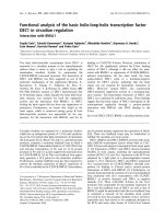
is shown in Figure 1. As stated earlier, each reaction
norm surface corresponds to a specific genetic effect.
Thus, if a QTL is at work, the genetic effects produce
different surfaces defined by distinct sets of model para-
meters corresponding to different genotypes.
Likelihood
We consider a backcross design with o ne QTL. Exten-
sions to more complicated designs and the two-QTL

case, as in [13], are straightforward. Assume a backcross
plant population of size n with a single QTL affecting
the phenotypic trait of photosynthetic rate. The photo-
synthetic rate for each progeny i (i =1, ,n)ismea-
sured at different irradiance ( s = 1, , S)and
temperature (t = 1, , T ) levels. This choice of variables
is adopted for consistency in later discussions as we will
be working with spatio-temporal covariance models.
The set of phenotype measurements or observations can
be written in vector form as
y
ii i
i
yyT
yS
= [ ( , ), , ( , ),
,[ ( , ),
11 1
1
irradiance 1

, ( , ) ,yST
i
’
irradiance S
 
(3)
0
100
200

300
15
20
25
30
0
0.5
1.0
1.5
2.0
Irradiance (I)
Temperature (T)
Photosynthetic Rate (P)
Figure 1 Reaction norm surface of photosynthetic rate as a function of irradiance and temperature. Model is based on equations (1) and
(2) with parameters (a, P
m
(20), θ) = (0.02, 1, 0.9). Adapted from [13].
Yap et al. BMC Plant Biology 2011, 11:23
/>Page 3 of 13
The proge ny are genotyped for molecular markers to
construct a genetic linkage map for the segregating QTL
in the population. This means that the genotypes of the
markers are observed and will be used, along with the
phenotype measurements, to predict the QTL. With a
backcross design, the QTL has two possible genotypes
(as do the markers) which shall be indexed by k =1,2.
The likelihood function based on the phenotype and
marker data can be formulated as
Lpf
ki

k
ki
i
n
() ( | )
|
ΩΩ=
⎡
⎣
⎢
⎢
⎤
⎦
⎥
⎥
=
=
∑
∏
1
2
1
y
(4)
where p
k|i
is the conditional probability of a QTL gen-
otype given the genotype o f a marker interval for pro-
geny i. We ass ume a multivariate normal density for the
phenotype vector y

i
with genotype-specific means
 

kk k
k
T
S
= [ ( , ), , ( , ),
,[ ( , ),
11 1
1
irradiance 1
 
, ( , )’,

k
ST
irradiance S

(5)
and covariance matrix Σ = cov(y
i
).
Mean and Covariance Models
The mean vector for photosynthetic rate in (5) can be
modeled using equations (1) and (2) as






k
kmk
k
kkkmk
k
st
sP
bsP
(, )=
+
−
−
2
4
2
2
(6)
Where b
k
= a
k
s + P
mk
,
Pt
PPttT
tT
mk

mk
()
()() *
*
=
≥
<
⎧
⎨
⎪
⎩
⎪
20
0
(7)
Pt
tT
T
()
*
*
=
−
−20
and k =1,2.
Wu et al. [13] used a separable structure (Mitchell
et al., 2005) for the ST × ST covariance matrix Σ as
ΣΣΣ
AR()112
=⊗

(8)
where Σ
1
and Σ
2
are the (S×S)and(T×T)covariance
matrices among different irradiance and temperature
levels, respectively, and ⊗ is the Kronecker product
operator. Note that Σ
1
and Σ
2
areuniqueonlyupto
multiples of a constant be cause for some |c| > 0, cΣ
1
⊗
(1/c)Σ
2
= Σ
1
⊗ Σ
2
. Each of Σ
1
and Σ
2
is modeled using
an AR(1) structure with a common error variance, s
2
,

and correlation parameters r
k
(k = 1, 2):
Σ
k
kk
S
kk
S
k
S
k
S
=
⎡
⎣
⎢
⎢
⎢
⎢
⎢
⎤
⎦
⎥
⎥
⎥
⎥
⎥
−
−

−−




2
1
2
12
1
1
1




(9)
Separable covariance structures, however, cannot
model interaction effects of each reaction norm to tem-
perature and irradiance. Thus, there is a need for a
more general model for this purpose.
Yap et al. [14] proposed to use a data-driven nonpara-
metric covariance estimator in functional mapping. The
authors showed that using such estimator provides bet-
ter estimates for QTL location and mean model para-
meters when compared t o AR(1). Huang et al. [16]
showed that the nonparametric estimator works well for
large matrices. Functional mapping of reaction norms
when there are two environmental signals necessitates
the use of large covariance matrices tha t result from

Kronecker products of smaller matrices. Here, we are
interested in determining whether the nonparametric
covariance estimator of Yap et al. [14] will still work
well in this reaction norm setting.
It shoul d be noted that unlike parametric models, e.g.
AR(1), there are no parameters being estimated in the
nonparametric covariance estimator. The entries of the
matrix are determined based on the data. This is differ-
ent from a model-dependent covariance matrix model
with one parameter for each of its elements. Due to
over-parametrization, such a model may not lead to
convergence to yield reliable results.
Note that with (6)-( 9), Ω = Ω
1
∪ Ω
2
in (4), where Ω
1
={a
1
, P
m1
(20), θ
1
, s
2
, r
1
}andΩ
1

={a
2
, P
m2
(20), θ
2
, s
2
,
r
2
}. These model parameters may be estimated using
the ECM algorithm [17], but closed form solutions at
the CM-step are be very complicated. A more efficient
method is to use the Nelder-Mead simplex algorithm
[23] which can be easily implemented using softwares
such as Matlab.
Hypothesis Tests
The features of the surface landscape are important
because they can be used as a basis in formulating
hypothesis tests. Let H
0
and H
1
denote the null and
alternative hypotheses, respectively. Then the existence
of a QTL that determines the reaction norm curves can
be formulated as
HPP
mm01 21 1 2

20 20: , () (), ,
 
===
versus
Yap et al. BMC Plant Biology 2011, 11:23
/>Page 4 of 13
H
1
: at least one of the equalities
above does not hold
This means that if the reaction norm curves are di s-
tinct (in terms of their respective estimated parameters ),
then a QTL possibly exists. The estimated location of
the QTL is at the point at which the log-likelihood ratio
obtained using the null and alternative hypotheses is
maximal. Of course a slight difference in parameter esti-
mates does not automatically mean a QTL exists. The
significanc e of the results can be determi ned by p ermu-
tation tests [24] which involves a repeated application of
the functional mapping model on the data where the
phe notype and marker associations are broken to simu-
late the null hypothesis of no QTL. A significance level
is then obtained based on the maximal log-likelihood
ratio at each application to infer the presence or absence
of a QTL (see ref. [25 ] for more details). A procedure
describedinref.[26]canbeusedtotesttheadditive
effects of a QTL. Other hypotheses can be formulated
and tested such as the genetic control of the reaction
norm to each environmental factor, interaction effects
between environmental fa ctors on the phenotype, and

the marginal slope of the reaction norm with respect to
each environmental factor or the gradient of the reac-
tion norm itself. The reader is referred to Wu et al. [13]
for more details.
Spatio-Temporal Covariances
We investigate the use of parametric and nonseparabl e
spatio-temporal covariance structures in functional map-
ping of photosynthetic rate as a reaction norm to the
environmental factors irradiance and temperature. As
stated earlier, the main idea is to model irradiance as a
one-dimensional spatial variable and temperature as a
temporal variable. The choice of which environmental
signal is modeled as temporal or spatial is arbitrary. For
more about spatio-temporal modeling, we refer the
reader to [27,19].
Basic Ideas, Notation, and Assumptions
We consider a real-valued spatio-temporal random pro-
cess given by
Yst st d
d
(, ),(, ) ,∈× ∈
+
 
(10)
where observations are collected at coordinates
( , ),( , ), ,( , )st st s t
NN11 2 2
to characterize unobserved portions of the process.
This collection of coordinates are not necessarily
ordered fixed levels of each trait. We will only be

concerned with the case d = 1. Aside from those men-
tioned earlier, Y may also represent ozone levels, disease
incidence, ocean current patterns or water temperatures.
In our setting, Y represents photosynthetic rate.
If var (Y(s, t)) < ∞ for all (s, t) Î ℛ × ℛ,thenthe
covariance, cov (Y(s, t), Y(s + u, t + v)), where u and v
are spatial and temporal lags, respectively, exists. We
assume that the covariance is stationary in space and
time so that for some function C,
cov ( ( , ), ( , )) ( , ).Yst Ys ut v Cuv++=
(11)
This means that the covariance function C depends
only on the lags and not on the values of the coordi-
nates themselves. Stationarity is often assumed to allow
estimation of the covariance function from the data
[18]. We also assume that the covariance function is iso-
tropic which means that it depends only o n the absolute
lags and not in the direction or orientation of the coor-
dinates to each other. The covariances considered in
this paper are positive (semi-) definite as they satisfy the
following condition: for any (s
1
, t
1
), , (s
k
, t
k
) Î ℛ ×
ℛ, any real coefficients a

1
, . , a
k
, and any positive inte-
ger k,
aaC s s t t
i
j
k
i
k
ji ji j
==
∑∑
−−≥
11
0(,)
(12)
Note that C(u,0)andC(0, v)correspondtopurely
spatial and purely temporal covariance functions,
respectively.
In spatio-temporal analysis, the ultimate goal is opti-
mal prediction (or kriging) of an un-observed part of
the random process Y(s, t) using an appropriate covar-
iance function model. We utilize a covariance model to
calculate the mixture likelihood associated with func-
tional mapping.
Separable and Nonseparable Covariance Structures
Separable Covariance Structures
A covariance function C(u, v|θ) of a spatio-temporal

process is separable if it can be expressed as
Cu v C u C v(, | ) ( | ) (| )

=
1122
(13)
where C
1
(u|θ
1
)andC
2
(v|θ
2
) are purely spatial and
purely temporal covariance functions, respectively, and θ
=(θ
1
, θ
2
)’. This representation implies that the observed
joint process ca n be see n as a product of two indepen-
dent spatial and temporal processes.
A more general definition for separability is as a Kro-
necker product (equation (8)). From equation (8), it can be
shown that
ΣΣΣ
AR()1
1
1

1
2
1−−−
=⊗
and
||||||
()
ΣΣΣ
AR
dd
11 2
21
=
,
Yap et al. BMC Plant Biology 2011, 11:23
/>Page 5 of 13
where |·| denotes the determinant of a matrix; d
1
and d
2
are the dimensions of Σ
1
and Σ
2
, respectively. This illus-
trates the computational advantage of using separable
models in likelihood estimation where the inverse and
determinant of the covariance matrix are calculated. For a
large covariance matrix of dimension UV, its inverse can
be calculated from the inverses of its Kronecker compo-

nent matrices, Σ
1
and Σ
2
, with dimensions U and V,
respectively. Thus, the inversion of a 100 × 100 matrix, for
example, may only require the inversion of two 10 × 10
matrices. A similar argument can be used for the determi-
nant. Σ
AR(1)
can be put in the form (13) as
Cu v
uv
uv
(, | , , )
,
  

2
12
2
1
2
2
4
12
=
=
.
(14)

where u =1, ,U , v =1, ,V. Note that this model
assumes e quidistant o r regularly spaced coordinates.
Thus, two con secutive or closest neighbor coordinates
will have th e same correlation structure as another even
if their respective distances are different. A more appro-
priate model might be
Cu v ab
ua vb
(, | , , , , )
//
 
2
12
4
12
=
(15)
where a and b are scale parameters. In this model, the
scale paramete rs correct for the uneven distance s
between coordinates.
Nonseparable Covariance Structures
Here, we present some nonseparable covariance models
that were deriv ed in two differen t ways. The details of
the derivation are omitted as they are rather compli-
cated and lengthy.
The following nonseparable covariance models were
derivedbyCressieandHuang[18]usingtheFourier
transform of the spectral density and by utilizing Boch-
ner’s Theorem [28]:
Cu v

av
bu
av
(, )
()
exp ,
=
+
×−
+
⎛
⎝
⎜
⎜
⎞
⎠
⎟
⎟

2
22
22
22
1
1
(16)
Cu v
av
av b u
(, )

(| | )
(| | ) | |
=
+
++

2
222
1
1
(17)
Cu v a v b u
cv u
( , ) exp( | | | | )
exp( | || | ),
=−−
×−

222
2
(18)
where a, b ≥ 0 are scaling parameters of time and
space, respectively; c ≥ 0 is an interaction parameter of
time and space, and s
2
= C(0, 0) ≥ 0. Note that when c
= 0, (18) reduces to a separable model.
Gneiting [27] developed an approach that can produce
nonseparable covariance models without relying on
Fourier transform pairs. One such model is

Cu v
av
bu
av
(, )
(| | )
exp
||
(| | )
,
=
+
×−
+
⎛
⎝
⎜
⎜
⎞
⎠
⎟
⎟




2
2
2
2

1
1
(19)
with (u, v) Î ℛ × ℛ and where a, b > 0 are s caling
param eters of space and time, respectively; a, b Î (0, 1]
are smoothness parameters of space and time, respec-
tively; g 0[1]; τ ≥ 1/2; and s
2
≥ 0. g is a space-time inter-
action parameter which implies a separable structure
when 0 and a nonseparable st ructure otherwise. Increas-
ing values of g indicates strengthening spatio-temporal
interaction.
Computer Simulation
We investigated the performances of the following non-
separable covariances structures that were presented in
the preceding section
Cuv
av
bu
av
1
2
22
22
22
1
1
(, )
()

exp ,
=
+
×−
+
⎛
⎝
⎜
⎜
⎞
⎠
⎟
⎟

(20)
Cuv
av
av b u
2
2
222
1
1
(, )
(| | )
(| | ) | |
,=
+
++


(21)
Cuv
av
bu
av
3
2
2
1
1
(, )
(| | )
exp
||
(| | )
,
/
=
+
×−
+
⎛
⎝
⎜
⎜
⎞
⎠
⎟
⎟



(22)
where a, b ≥ 0; g Î 0[1] and s
2
>0.C
1
and C
2
corre-
spond to (16) and (17), respectively, and C
3
is a special
case of (19) with a = 1/2, b = 1/2 and τ =1.
We generated photosynthetic rate data using these
nonseparable covariances to simulate interaction effects
between the two environmenta l signals in functional
mapping of a reaction norm. The generated data was
analyzed using the nonpa rametric estimator Σ
NP
pro-
posed by Yap et al. [14] using an L
2
penalty, and Σ
AR(1)
(equation (8)). Note that the underlying covariance
structures were very different from the assumed model,
Σ
AR(1)
, and we therefore expected to get biased esti-
mates. The issue we wanted to address was the extent

Yap et al. BMC Plant Biology 2011, 11:23
/>Page 6 of 13
to which the bias cannot be ignored and an alternative
estimator such as Σ
NP
may be more appropriate.
Covariance fit was assessed using entropy (L
E
)and
quadratic (L
Q
) losses:
Lm
E
(,) ( ) logΣΣ ΣΣ ΣΣ=− −
−−
tr
11
and
LI
Q
(,) ( )ΣΣ Σ Σ=−
−
tr
12
where
ˆ
Σ
is the estimate of the true underlying covar-
iance Σ [14,16,29-31]. Each loss function is 0 when

ˆ
ΣΣ=
and large values suggest significant bias.
Using a backcross design for t he QTL mapping popu-
lation, we rand omly generated 6 markers equally spaced
on a chromosome 100 cM long. One QTL was simu-
lated bet ween the fourth and fifth markers, 12 cM from
the fourth marker (or 72 cM from the leftmost marker
of the chromosome). The QTL had two possible geno-
types which determined two distinct mean photosyn-
thetic ra te reaction norm surfaces define d by equations
(1) and (2) (see also Figure 1 ). The surface parameters
for each genotype were ( a
1
, P
m1
(20), θ
1
) = (0.02, 2, 0.9)
and (a
2
, P
m2
(20), θ
2
) = (0.01, 1.5, 0.9). Phenotype obser-
vations were obtained by sampling from a multivariate
normal distribution with mean surface based on irradi-
ance and temperature levels of {0, 50, 100, 200, 300}
and {15, 20, 25, 30}, respectively, and covariance matrix

C
l
( u, v), l = 1, 2, 3 with a = 0.50, b =0.01forC
1
, a =
1.00, b =0.01forC
2
, a =1.00,b =0.01,c =0.60forC
3
and s
2
= 1.00 for all three covariances.
Figure 2 shows the reaction norm surfaces of photo-
synthetic rate as functions of irradiance and temperature
that were used in the simulation. Within the considered
domain of values for ir radiance and temperature, one
surface lies above the other. These surfaces differ only
in terms of the a
2
and P
m1
(20) parameters.
The functional mapping model was applied to the
marker and phenotype data with n = 200, 400 samples.
The surface defined by equations (1) and (2) was used
as mean model with Σ
NP
and Σ
AR(1)
as cova riance mod-

els to analyze the data generated using C
l
(u, v). 100
simulation runs were carried out and the averages on all
runs of the estimated QTL location, mean parameter
estimates, entropy and quadratic losses, including the
respective Monte carlo standard errors (SE), were
recorded. Tables 1 and 2 present the results of these
simulat ions. The results show that using Σ
NP
yields rea-
sonably accurate and precise parameter estimates. The
results for Σ
AR(1)
are similar to Σ
NP
except that the aver-
age losses, given by L
E
and L
Q
,areinflatedforC
1
and
C
2
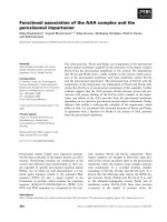
. Figure 3 shows box plots of the log-likelihood values
under the alternative model. These plots reveal biased
estimates of C
1

and C
2
by Σ
AR(1)
and the degrees of bias
are consistent with the average losses. The results for
the log-likelihood values under the null model are very
similar but are not shown. We also provided the covar-
iance and correspond ing contour plots of C
l
(u, v), l =1,
2, 3 and the Σ
AR(1)
estimates of these in Figure 4 a nd 5.
We only provided plots for C
l
(u, v), l =1,2,3andΣ
AR
(1)
to illustrate the behavior of these parametric models.
We did not include plots for the estimated Σ
NP
becaus e
there are no parametric estimates for this model and we
did not record all elements of the estimated Σ
NP
in the
simulation runs.
We conducted further simulations using C
1

as the
underlying covariance structure of the data with n =
400. This was the case where Σ
AR(1)
performed the
worst. We considered two scenarios: increased variance
parameter, s
2
, or increased irradiance and temperature
levels (finer grid). That is,
1. s
2
= 2, 4 with irradiance and temperature levels of
{0, 50, 100, 200, 300} and {15, 20, 25, 30},
respectively.
2. s
2
= 1, 2 with irradiance and temperature levels of
{0, 50, 100, 150, 200, 250, 300} and {15, 18, 21, 24,
27, 30}, respectively.
We included an analysis of the simulated data using
C
1
as the covariance model to ensure the results are not
false-positives. The results of the simulation are shown
in Tables 3 and 4. The tables include columns for the
log- likelihood values under the null (H
0
) and alternative
(H

1
) hypotheses as well as the maximum of the log-like-
lihood ratio (maxLR). MaxLR is used in permutation
tests to assess significance of QTL existence (see Section
2.3). Under scenarios (1) or (2), i.e. increased variance
parameter s
2
or increased irradiance and temperature
levels, using Σ
NP
yields significantly more accurate and
precise estimates of the QTL location compared to Σ
AR
(1)
:InTable3,whens
2
= 4, the estimates of the true
QTL location of 72 we re 71.64 and 74.20 for NP and
Σ
AR(1)
, respectively; In Table 4, when s
2
=2,theesti-
mates were 72.13 and 78.44. Although for Σ
AR(1)
, maxLR
appears to be more accurate, the log- likelihood ratios
are s till significantly different from the estimates given
by C
1

. Again, this is reflected in the inflated average
losses. Note that the maxLR estimates are larger for Σ
AR
(1)
when compared to those f or Σ
NP
. We do not expect
this to be always the case. In other instances, the maxLR
estimates for Σ
AR(1)
may be smaller than those for Σ
NP
.
However, in those instances, we expect the maxLR esti-
mates for Σ
NP
to still be more accurate and precise than
Yap et al. BMC Plant Biology 2011, 11:23
/>Page 7 of 13
0
100
200
300
10
20
30
0
1
2
3

4
0
100
200
300
10
20
30
0
1
2
3
4
0
200
400
15
20
25
30
0
1
2
3
4
0
100
200
300
10

20
30
0
1
2
3
4
Figure 2 Reaction norm surfaces of photosynthetic rate as functions of irradiance and temperature. Models are based on equa tions (1)
and (2) with parameters (a
1
, P
m1
(20), θ
1
) = (0.02, 2, 0.9) and (a
2
, P
m2
(20), θ
2
) = (0.01, 1.5, 0.9) as used in the simulation.
Table 1 Averaged QTL position, mean curve parameters, entropy and quadratic losses and their standard errors (given
in parentheses) for two QTL genotypes in a backcross population under different sample sizes (n) based on 100
simulation replicates (Σ
NP
)
QTL QTL genotype 1 QTL genotype 2
Covariance n Location
ˆ


1
ˆ
()P
m1
20
ˆ

1
ˆ

2
ˆ
()P
m2
20
ˆ

2
L
E
L
Q
C
1
200 71.68 0.02 2.02 0.90 0.01 1.52 0.88 1.04 2.03
(0.28) (0.00) (0.01) (0.00) (0.00) (0.02) (0.01) (0.01) (0.02)
400 72.16 0.02 2.00 0.90 0.01 1.52 0.88 0.53 1.06
(0.23) (0.00) (0.01) (0.00) (0.00) (0.01) (0.01) (0.00) (0.01)
C
2

200 71.88 0.02 2.00 0.90 0.01 1.53 0.88 1.00 1.96
(0.29) (0.00) (0.01) (0.00) (0.00) (0.01) (0.01) (0.01) (0.02)
400 71.92 0.02 2.00 0.90 0.01 1.52 0.89 0.52 1.02
(0.17) (0.00) (0.01) (0.00) (0.00) (0.01) (0.01) (0.00) (0.01)
C
3
200 72.12 0.02 2.01 0.89 0.01 1.54 0.87 0.88 1.70
(0.37) (0.00) (0.01) (0.01) (0.00) (0.02) (0.01) (0.01) (0.02)
400 72.08 0.02 2.01 0.90 0.01 1.52 0.89 0.48 0.94
(0.20) (0.00) (0.01) (0.00) (0.00) (0.01) (0.01) (0.00) (0.01)
True: 72.00 0.02 2.00 0.90 0.01 1.50 0.90
Yap et al. BMC Plant Biology 2011, 11:23
/>Page 8 of 13
Table 2 Averaged QTL position, mean curve parameters, entropy and quadratic losses and their standard errors (given
in parentheses) for two QTL genotypes in a backcross population under different sample sizes (n) based on 100
simulation replicates (Σ
AR(1)
)
QTL QTL genotype 1 QTL genotype 2
Covariance n Location
ˆ

1
ˆ
()P
m1
20
ˆ

1

ˆ

2
ˆ
()P
m2
20
ˆ

2
L
E
L
Q
C
1
200 72.32 0.02 2.03 0.90 0.01 1.53 0.87 19.43 681.78
(0.45) (0.00) (0.01) (0.01) (0.00) (0.02) (0.01) (0.07) (6.16)
400 71.72 0.02 2.03 0.90 0.01 1.51 0.89 19.45 684.11
(0.27) (0.00) (0.01) (0.00) (0.00) (0.01) (0.01) (0.05) (4.40)
C
2
200 71.96 0.02 2.01 0.90 0.01 1.55 0.87 4.83 58.60
(0.34) (0.00) (0.01) (0.00) (0.00) (0.02) (0.01) (0.02) (1.01)
400 71.84 0.02 2.01 0.90 0.01 1.52 0.89 4.83 58.61
(0.20) (0.00) (0.01) (0.00) (0.00) (0.01) (0.01) (0.02) (0.77)
C
3
200 72.00 0.02 2.01 0.89 0.01 1.54 0.87 0.60 1.51
(0.35) (0.00) (0.01) (0.01) (0.00) (0.02) (0.01) (0.00) (0.10)

400 71.96 0.02 2.01 0.89 0.01 1.52 0.89 0.60 1.43
(0.22) (0.00) (0.01) (0.00) (0.00) (0.01) (0.01) (0.00) (0.08)
True: 72.00 0.02 2.00 0.90 0.01 1.50 0.90
−1500
−1100
−700
−300
n=200
log−likelihood, H
1

−3000
−2000
−1000
n=400
log−likelihood, H
1
−1300
−950
−600
log−likelihood, H
1
−2500
−2100
−1700
−1300
log−likelihood, H
1
−1700
−1400

−1100
log−likelihood, H
1
−3300
−2950
−2600
log−likelihood, H
1
NP
C
1

AR(1)
NP
C
1

NP
C
2

NP
C
2

NP
C
3

NP

C
3

AR(1)
AR(1)
AR(1)
AR(1) AR(1)
Figure 3 Boxplots of the values of the log-likelihood under the alternative model, H
1
. Significantly biased estimates by Σ
AR(1)
are apparent
for C
1
.
Yap et al. BMC Plant Biology 2011, 11:23
/>Page 9 of 13
those for Σ
AR(1)
, unless the true underlying covariance
structure is Σ
AR(1)
, which is not likely.
Discussion
In this paper, we studied the covariance model in func-
tional mapping of photosynthetic rate as a reaction
norm to irra diance and temperature as environmental
signals. In the presence of interaction between the two
signal s simulated by nonseparable covariance structures,
our analysis showed that Σ

NP
is a more reliable estima-
tor than Σ
AR(1)
particularly in QTL location estimation.
The advantage of Σ
NP
over Σ
AR(1)
is greater when the
variance of the reaction norm process and the number
of signal levels increase.
Σ
NP
was developed in the context of a one dimen-
sional (longitudinal) vector which has an ordering of
variables. The p henotype vector we considere d here
consists of observations based on two levels of irradi-
ance and temperature measurements, i.e.,
y
ii i
i
yyT
yS
= [ ( , ), , ( , ),
,[ ( , ),
11 1
1
irradiance 1


, ( , )’,yST
i
irradiance S
 
(23)
This vector has no natural ordering like in longitudi-
nal data. However, our simulation results still suggest
that Σ
NP
can be directly applied to observations that
have no variable ordering such as (23). The process by
which Σ
NP
was obtained in Yap et al. [14] was based on
non-mixture type of longitudinal covariance estimators.
This process is flexible and can p otentially accommo-
date other estimators that can handle unordered data or
are invariant to variable permutations. See for example
0
100
200
300
0
5
10
15
0
0.5
1
|u|

TRUE NONSEPARABLE COVARIANCE
|v|
C
1
(u,v)
0
1
2
3
0
1
2
3
0
0.5
1
AR(1)
0
100
200
300
0
5
10
15
0
0.5
1
|u|
|v|

C
2
(u,v)
0
1
2
3
0
1
2
3
0
0.5
1
0
100
200
300
0
5
10
15
0
0.5
1
|u|
|v|
C
3
(u,v)

0
1
2
3
0
1
2
3
0
0.5
1
Figure 4 Covariance plots. Plots of C
l
, l = 1, 2, 3 versus irradiance (|u|) and temperature (|v|) lags are on the left column. On the right column
are the estimates of C
l
by ∑
AR(1)
.
Yap et al. BMC Plant Biology 2011, 11:23
/>Page 10 of 13
the sparse permutation invariant covariance estimator
(SPICE) proposed by Rothman et al. [32].
In the presence of interactions, nonseparable covar-
iances can possibly be used in place of Σ
NP
,butthey
should closel y reflect the structure of the data. Unfortu-
nately, as with any parametric model, this is not often
the case. In fact, it is not even known whether the data

exhibits interactions or not. Before deciding on what
model to use, one might utilize tests for separability
[33,34]. If separable models a re appropriate, then there
are many options. Otherwise, it is difficult to choose
from a number of complex nonsep arable covari ances
because there are no a vailabl e general guidelines as yet
that can help one decide which model to use. The cov-
ariance C
3
that was used in the simulations had an easy
to interpret interaction parameter g Î 0[1]. However,
despite an interaction “strength ” of g = 0.6, the separable
model, Σ
AR(1)
, estimated the da ta generated by C
3
quite
well. Thus, the trade-o between using a nonseparable
model instead of a separable one may not be worth it.
Another option is to use separable approximations to
nonseparable covariances [35]. The nonseparable covar -
iances that we considered were assumed to be stationary
and isotropic. These two assumptions may not always
hold for real data. Although not specifically addressed
here, using Σ
NP
may work f or data that do not satisfy
these assumptions.
Fina lly, we only consid ered two environmental signal s
with interactions: irradiance and temperature. However,

the reaction norm of photosynthetic rate is a very com-
plex process because there are really more environmen-
tal signals at play other than these two. Theoretically,
the spatial domain of spatio-temporal nonseparable cov-
ariance models can be extended to more than one
0 100 200 300
0
5
10
15
|u|
|v|
TRUE NONSEPARABLE COVARIANCE
0 1 2 3
0
1
2
3
AR(1)
0 100 200 300
0
5
10
15
|u|
|v|
0 1 2 3
0
1
2

3
0 100 200 300
0
5
10
15
|u|
|v|
0 1 2 3
0
1
2
3
C
1
(u,v)
C
2
(u,v)
C
3
(u,v)
Figure 5 Contour plots. Contour plots of C
l
, l = 1, 2, 3 on the left column. On the right column are the contour plots of the estimates of C
l
by
Σ
AR(1)
.

Yap et al. BMC Plant Biology 2011, 11:23
/>Page 11 of 13
dimensions i.e., d > 1 in (10). For example, a two
dimensional spatial domain models an area on a flat
surface while a three dimensional domain models space.
There are spatio-temporal models for these. However,
this extension cannot be used to increase the number of
signals in a reac tion norm unless the signals have the
same unit of measurement or one assumes separability
or no interaction among the signals. For example, car-
bon dioxide concentration cannot be a dded as a signal,
in addition to irradian ce and temperature, when model-
ing p hotosynthet ic rate as a reaction norm in the func-
tional mapping setting because it does not have the
same unit as i rradiance or temperature. Thus, it is diffi-
cult to simulate data from more than two signals with
interactions. However, Σ
NP
can theoretically handle cov-
ariance s associated with more than two signals that may
involve interactions. The computer code for the model
will be available from .
Table 3 Averaged QTL position, mean curve parameters, log-likelihood values, maximum log-likelihood ratios (maxLR),
entropy and quadratic losses and their standard errors (given in parentheses) for two QTL genotypes in a backcross
population based on 100 simulation replicates (C
1
with n = 400 and s
2
=2,4)
QTL QTL genotype 1 QTL genotype 2 log-likelihood

Covariance s
2
Location
ˆ

1
ˆ
()P
m1
20
ˆ

1
ˆ

2
ˆ
()P
m2
20
ˆ

2
H
0
H
1
maxLR L
E
L

Q
Σ
AR(1)
2 72.40 0.02 2.05 0.89 0.01 1.52 0.87 -5437 -5373 128.51 19.45 684.37
(0.44) (0.00) (0.01) (0.01) (0.00) (0.02) (0.01) (7.36) (7.31) (2.45) (0.05) (4.44)
4 74.20 0.02 2.11 0.88 0.01 1.52 0.84 -8175 -8141 65.55 19.44 683.82
(0.69) (0.00) (0.02) (0.01) (0.00) (0.03) (0.02) (7.32) (7.31) (1.80) (0.05) (4.46)
C
1
2 71.96 0.02 2.01 0.90 0.01 1.54 0.88 -4088 -4021 133.41 0.01 0.13
(0.29) (0.00) (0.01) (0.00) (0.00) (0.02) (0.01) (7.17) (7.16) (2.15) (0.00) (0.02)
4 71.96 0.02 2.03 0.89 0.01 1.57 0.86 -6822 -6788 69.07 0.01 0.13
(0.44) (0.00) (0.01) (0.01) (0.00) (0.03) (0.02) (7.16) (7.16) (1.57) (0.00) (0.02)
NP 2 72.16 0.02 2.01 0.89 0.01 1.54 0.87 -3967 -3912 109.79 0.53 1.05
(0.29) (0.00) (0.01) (0.00) (0.00) (0.02) (0.01) (6.87) (6.89) (1.66) (0.00) (0.01)
4 71.64 0.02 2.01 0.89 0.01 1.57 0.84 -6713 -6684 59.92 0.53 1.04
(0.49) (0.00) (0.01) (0.01) (0.00) (0.03) (0.02) (6.89) (6.93) (1.27) (0.00) (0.01)
True: 72.00 0.02 2.00 0.90 0.01 1.50 0.90
Table 4 Averaged QTL position, mean curve parameters, log-likelihood values, maximum log-likelihood ratios (maxLR),
entropy and quadratic losses and their standard errors (given in parentheses) for two QTL genotypes in a backcross
population based on 100 simulation replicates (C
1
with n = 400, increased irradiance and temperature levels, and
s
2
=1,2)
QTL QTL genotype 1 QTL genotype 2 log-likelihood
Covariance s
2
Location

ˆ

1
ˆ
()P
m1
20
ˆ

1
ˆ

2
ˆ
()P
m2
20
ˆ

2
H
0
H
1
maxLR L
E
L
Q
Σ
AR(1)

1 72.16 0.02 2.04 0.90 0.01 1.48 0.88 -1278 -1063 430.01 223 64090
(0.36) (0.00) (0.01) (0.00) (0.00) (0.01) (0.01) (14.01) (14.15) (4.78) (0.45) (261.88)
2 78.44 0.02 2.15 0.91 0.01 1.48 0.86 -6992 -6876 231.86 222 63923
(0.84) (0.00) (0.02) (0.00) (0.00) (0.02) (0.01) (14.08) (14.16) (3.62) (0.44) (257.89)
C
1
1 71.76 0.02 2.01 0.90 0.01 1.51 0.89 4913 5068 309.86 0.01 0.31
(0.18) (0.00) (0.00) (0.00) (0.00) (0.01) (0.00) (11.04) (11.10) (3.17) (0.00) (0.04)
2 71.76 0.02 2.01 0.90 0.01 1.52 0.88 -821.08 -743.76 154.64 0.01 0.31
(0.24) (0.00) (0.01) (0.00) (0.00) (0.01) (0.01) (11.10) (11.12) (2.22) (0.00) (0.04)
NP 1 71.73 0.02 2.01 0.90 0.01 1.51 0.89 5431 5537 212.64 2.34 4.55
(0.18) (0.00) (0.01) (0.00) (0.00) (0.01) (0.00) (11.22) (11.11) (2.20) (0.01) (0.03)
2 72.13 0.02 2.01 0.90 0.01 1.49 0.89 -336 -273 127.37 2.37 4.53
(0.34) (0.00) (0.01) (0.00) (0.00) (0.01) (0.01) (10.44) (10.42) (1.72) (0.01) (0.03)
True: 72.00 0.02 2.00 0.90 0.01 1.50 0.90
Yap et al. BMC Plant Biology 2011, 11:23
/>Page 12 of 13
Acknowledgements
This work is partially supported by NSF grant IOS-0923975, the Changjiang
Scholarship Award and “One-thousand Person Plan” Award at Beijing
Forestry University.
Author details
1
Department of Statistics, University of Florida, Gainesville, FL 32611 USA.
2
Department of Statistics, West Virginia University, Morgantown, WV 26506,
USA.
3
Center for Statistical Genetics, Pennsylvania State University, Hershey,
PA 17033, USA.

4
Center for Computational Biology, Beijing Forestry
University, Beijing 100083, PR China.
Authors’ contributions
JY participated in the design of the study, performed the statistical analysis,
and wrote the manuscript. YL, KD and JL participated in the statistical
analysis. RW conceived of the study, participated in its design and
coordination, and wrote the manuscript. All authors read and approved the
final manuscript.
Received: 21 November 2009 Accepted: 26 January 2011
Published: 26 January 2011
References
1. Via S, Gomulkievicz R, de Jong G, Scheiner SM, et al: Adaptive phenotypic
plasticity: Consensus and controversy. Trends in Ecology and Evolution
1995, 10:212-217.
2. Scheiner SM: Genetics and evolution of phenotypic plasticity. Annual
Reviews of Ecology and Systematics 1993, 24:35-68.
3. Schlichting CD, Smith H: Phenotypic plasticity: Linking molecular
mechanisms with evolutionary outcomes. Evolutionary Ecology 2002,
16:189-201.
4. West-Eberhard MJ: Developmental Plasticity: An Evolution Oxford University
Press, New York; 2003.
5. Wu RL: The detection of plasticity genes in heterogeneous
environments. Evolution 1998, 52:967-977.
6. Wu RL, Grissom JE, McKeand SE, O’Malley DM: Phenotypic plasticity of fine
root growth increases plant productivity in pine seedlings. BMC Ecology
2004, 4:14.
7. de Jong G: Evolution of phenotypic plasticity: Patterns of plasticity and
the emergence of ecotypes. New Phytologist 2005, 166:101-117.
8. Kingsolver JG, Izem R, Ragland GJ: Plasticity of size and growth in

fluctuating thermal environments: comparing reaction norms and
performance curves. Integrative and Comparative Biology 2004, 44:450-460.
9. Angilletta MJ Jr, Sears MW: Evolution of thermal reaction norms for
growth rate and body size in ectotherms: an introduction to the
symposium. Integrative and Comparative Biology 2004, 44:401-402.
10. Yap JS, Wang CG, Wu RL: A simulation approach for functional mapping
of quantitative trait loci that regulate thermal performance curves. PLoS
ONE 2007, 2(6):e554.
11. Stratton D: Reaction norm functions and QTL-environment interactions
for flowering time in Arabidopsis thaliana. Heredity 1998, 81:144-155.
12. Kirkpatrick M, Heckman N: A quantitative genetic model for growth,
shape, reaction norms, and other infinite-dimensional characters. Journal
of Mathematical Biology 1989, 27:429-450.
13. Wu J, Zeng Y, Huang J, Hou W, Zhu J, Wu RL: Functional mapping of
reaction norms to multiple environmental signals. Genetical Research
2007, 89:27-38.
14. Yap JS, Fan J, Wu RL: Nonparametric covariance estimation in functional
map-ping of quantitative trait loci. Biometrics 2009, 65
:1068-1077.
15. Pourahmadi M: Joint mean-covariance models with applications to
longitudinal data: Unconstrained parameterisation. Biometrika 1999,
86(3):677-690.
16. Huang J, Liu N, Pourahmadi M, Liu L: Covariance selection and estimation
via penalised normal likelihood. Biometrika 2006, 93:85-98.
17. Meng X-L, Rubin D: Maximum likelihood estimation via the ECM
algorithm: A general framework. Biometrika 1993, 80:267-278.
18. Cressie N, Huang H-C: Classes of nonseparable, spatio-temporal
stationary covariance functions. Journal of the American Statistical
Association 1999, 94:1330-1340.
19. Gneiting T, Genton M, Guttorp P: Geostatistical space-time models,

stationary, separability and full symmetry. In Statistical Methods for Spatio-
temporal Systems (Monographs on Statistics and Applied Probability). Edited
by: Finkenstadt B, Held L, Isham V. Chapman 2006:.
20. Wolf JB: The geometry of phenotypic evolution in developmental
hyperspace. Proceedings of the National Academy of Sciences of the USA
2002, 99:15849-15851.
21. Wu RL, Ma C-X, Casella G: Statistical Genetics of Quantitative Traits: Linkage,
Maps, and QTL Springer-Verlag, New York; 2007.
22. Thornley JHM, Johnson IR: Plant and Crop Modelling: A Mathematical
Approach to Plant and Crop Physiology Clarendon Press, Oxford; 1990.
23. Nelder J, Mead R: A simplex method for function minimization. Computer
Journal 1965, 7:308-313.
24. Doerge RW, Churchill GA: Permutation tests for multiple loci affecting a
quantitative character. Genetics 1996, 142:285-294.
25. Ma C, Casella G, Wu RL: Functional mapping of quantitative trait loci
underlying the character process: A theoretical framework. Genetics 2002,
161:1751-1762.
26. Wu RL, Ma C-X, Lin M, Casella G: A general framework for analyzing the
genetic architecture of developmental characteristics. Genetics 2004,
166:1541-1551.
27. Gneiting T: Nonseparable, stationary covarience functions for space-time
data. Journal of the American Statistical Association 2002, 97:590-600.
28. Bochner S: Harmonic Analysis and the Theory of Probability University of
California Press, Berkley and Los Angeles; 1955.
29. Wu WB, Pourahmadi M: Nonparametric estimation of large covariance
matrices of longitudinal data. Biometrika 2003, 90:831-844.
30. Huang J, Liu L, Liu N: Estimation of large covariance matrices of
longitudinal data with basis function approximations. Journal of
Computational and Graphical Statistics 2007, 16:189-209.
31. Levina E, Rothman A, Zhu J: Sparse estimation of large covariance

matrices via a nested lasso penalty. Annals of Applied Statistics 2008,
2:245-263.
32. Rothman A, Bickel P, Levina E, Zhu J: Sparse permutation invariant
covariance estimation. Electronic Journal of Statistics 2008, 2:494-515.
33. Mitchell MW, Genton MG, Gumpertz ML: Testing for separability of space-
time covariences. Envirometrics 2005, 16:819-831.
34. Fuentes M: Testing separability of spatial-temporal covariance functions.
Journal of Statistical Planning and Inference 2005, 136:447-466.
35. Genton M: Separable approximations of space-time covariance matrices.
Envirometrics 2007, 18:681-695.
doi:10.1186/1471-2229-11-23
Cite this article as: Yap et al.: Functional mapping of reaction norms to
multiple environmental signals through nonparametric covariance
estimation. BMC Plant Biology 2011 11:23.
Submit your next manuscript to BioMed Central
and take full advantage of:
• Convenient online submission
• Thorough peer review
• No space constraints or color figure charges
• Immediate publication on acceptance
• Inclusion in PubMed, CAS, Scopus and Google Scholar
• Research which is freely available for redistribution
Submit your manuscript at
www.biomedcentral.com/submit
Yap et al. BMC Plant Biology 2011, 11:23
/>Page 13 of 13