COASTAL AQUIFER MANAGEMENT: monitoring, modeling, and case studies - Chapter 3 ppsx

CHAPTER 3
MODFLOW-Based Tools for Simulation of
Variable-Density Groundwater Flow
C.D. Langevin, G.H.P. Oude Essink, S. Panday, M. Bakker,
H. Prommer, E.D. Swain, W. Jones, M. Beach, M. Barcelo
1. INTRODUCTION
Most scientists and engineers refer to MODFLOW [McDonald and
Harbaugh, 1988; Harbaugh and McDonald, 1996; Harbaugh et al., 2000] as
the computer program most widely used for constant-density groundwater
flow problems. The success of MODFLOW is largely attributed to its
thorough documentation, modular structure, which makes the program easy
to modify and enhance, and the public availability of the software and source
code. MODFLOW has been referred to as a “community model,” because of
the large number of packages and utilities developed for the program [Hill et
al., 2003]. In recent years, the MODFLOW code has been adapted to
simulate variable-density groundwater flow. Because MODFLOW is so
widely used, these variable-density versions of the code are rapidly gaining
acceptance by the modeling community.
To represent variable-density flow in MODFLOW, the flow equation
is formulated in terms of equivalent freshwater head. With this approach, the
finite-difference representation is rewritten so that fluid density is isolated
into mathematical terms that are identical in form to source and sink terms.
These “pseudo-sources” can then be easily incorporated into the matrix
equations solved by MODFLOW. Weiss [1982] was one of the first to recast
the groundwater flow equation in terms of equivalent freshwater head and
introduce the concept of a pseudo-source. Lebbe [1983] used a similar
approach to develop a variable-density version of the MOC code [Konikow
and Bredehoeft, 1978]. Maas and Emke [1988] were among the first to
incorporate variable-density flow into MODFLOW. The approach was

improved by Olsthoorn [1996] to account for inclined model layers. These
initial studies allowed for fluid density to vary in space, but not in time.
Recently, solute transport codes have been linked directly with MODFLOW
to represent the transient effects of an advecting and dispersing solute
© 2004 by CRC Press LLC
Coastal Aquifer Management
50
concentration field on variable-density groundwater flow patterns. These
MODFLOW-based codes are being applied to numerous hydrologic
problems involving variable-density groundwater flow.
Descriptions and applications of four of the commonly used
MODFLOW-based computer codes are presented in this chapter. The four
codes (SEAWAT, MOCDENS3D, MODHMS, and the Sea Water Intrusion
Package for MODFLOW-2000) have been applied to case studies and have
been documented and tested with variable-density benchmark problems. The
first three programs represent advective and dispersive solute transport. The
fourth program uses a non-dispersive, continuity of flow approach to
simulate movement of multiple density isosurfaces.
2. SEAWAT
C.D. Langevin, H. Prommer, E.D. Swain
The SEAWAT computer program is designed to simulate a wide
range of hydrogeologic problems involving variable-density groundwater
flow and solute transport. The SEAWAT code has been applied worldwide
to evaluate such problems as saltwater intrusion, submarine groundwater
discharge, aquifer storage and recovery, brine migration, and coastal wetland
hydrology. The source code, documentation, and executable computer
program are available to the public at the USGS web page.
1

This section provides a brief description of the SEAWAT program

and presents applications of SEAWAT to geochemical modeling and
integrated surface water and groundwater modeling. Additional information,
including the SEAWAT documentation, is available on the accompanying
CD.
2.1 Program Description
SEAWAT was designed by combining MODFLOW-88 and
MT3DMS into a single program that solves the coupled variable-density
groundwater flow and solute-transport equations [Guo and Bennett, 1998;
Guo and Langevin, 2002]. The flow and transport equations are coupled in
two ways. First, the fluid velocities that result from solving the flow
equation are used in the advective term of the solute-transport equation.
Second, the solute-transport equation is solved, and an equation of state is
used to calculate fluid densities from the updated solute concentrations.
These fluid densities are then used directly in the next solution to the
variable-density groundwater flow equation.


1

© 2004 by CRC Press LLC
MODFLOW-Based Tools
51
The variable-density groundwater flow equation solved by
SEAWAT is formulated using equivalent freshwater head as the principal
dependent variable. In this form, the equation is similar to the constant-
density groundwater flow equation solved by MODFLOW. Thus, with
minor modifications, MODFLOW routines are used to represent variable
density groundwater flow. Modifications include conservation of fluid mass,
rather than fluid volume, and the addition of relative density difference
terms, or pseudo-sources. The procedure for solving the variable-density

flow equation is identical to the procedure implemented in MODFLOW.
Matrix equations are formulated for each iteration, and a solver approximates
the solution. Modifications are not required for the MT3DMS routines that
solve the transport equation.
Like MT3DMS, SEAWAT divides simulations into stress periods,
flow timesteps, and transport timesteps. The lengths for stress periods and
flow timesteps are specified by the user; however, the time lengths for
transport timesteps are calculated by the program based on stability criteria
for an accurate solution to the transport equation. Because flow and
transport are coupled in SEAWAT, either explicitly or implicitly, the flow
and transport equations are solved for each transport timestep. This
requirement does not apply for simulations with standard MODFLOW and
MT3DMS because, in those cases, concentrations do not affect the flow
field.
Output from SEAWAT consists of equivalent freshwater heads, cell-
by-cell fluid fluxes, solute concentrations, and mass balance information.
This output is in standard MODFLOW and MT3DMS format, and most
publicly and commercially available software can be used to process
simulation results. For example, animations of velocity vectors and solute
concentrations can be prepared using the U.S. Geological Survey’s Model
Viewer program [Hsieh and Winston, 2002], and post-processing programs
such as MODPATH [Pollock, 1994] can be used to perform particle tracking
using SEAWAT output.
The U.S. Geological Survey actively supports the SEAWAT
program. As new packages, processes, and utilities are added to the
MODFLOW and MT3DMS programs, these improvements are incorporated
into SEAWAT. For example, a new version of SEAWAT, which is based on
MODFLOW-2000, was recently developed.
2.2 Reactive Transport Modeling with PHREEQC and SEAWAT
Two disciplines, namely, reactive transport modeling and variable-

density flow modeling, have received significant attention over the past two
decades. Well-known representatives of the former class of models are, for
example, MIN3P [Mayer et al., 2002], GIMRT/CRUNCH [Steefel, 2001],
© 2004 by CRC Press LLC
Coastal Aquifer Management
52
PHREEQC [Parkhurst and Appelo, 1999], PHAST [Parkhurst et al., 1995],
HydroBioGeoChem [Yeh et al., 1998], and some MODFLOW/MT3DMS-
based models such as RT3D [Clement, 1997] and PHT3D [Prommer et al.,
2003].
In most cases the separation of the two disciplines is well justified,
because (i) density gradients are small enough to be of negligible influence
on the reactive transport of multiple solutes or (ii) reactions, in particular
water-sediment interactions such as mineral dissolution/precipitation and/or
sorption, have a minor effect on the density of the aqueous phase. However,
specific cases exist where transport phenomena can only be accurately
described by considering simultaneously both variable density and reactive
processes. For example, Zhang et al. [1998] were only able to explain the
differential downward movement of a lithium (Li
+
) and a bromide (Br
−
)
plume at Cape Cod through multi-species transport simulations that
considered the variable density of the plume(s) and lithium sorption.
Furthermore, Christensen et al. [2001, 2002] demonstrated the interactions
between reactive processes and density variations for (i) a controlled
seawater intrusion experiment, where seawater was forced inland by
pumping, thereby undergoing reactions such as Na/Ca exchange, calcite
dissolution-precipitation, sulfate-reduction, and FeS precipitation, and (ii) for

a landfill leachate plume, where the density influences the distribution of the
redox-species and buffering reactions by Fe and Mn hydroxides. The
ongoing project to combine SEAWAT with the geochemical model
PHREEQC-2 was initially motivated by the desire to simulate and quantify
reactive changes that occur as a result of tidally induced, variable density
flow near the aquifer/ocean interface.
The governing equation for both transport and reactions of the i
th

(mobile) aqueous species/component, solved by the coupled model, is:
()
,
ii
ireaci
CC
DvCr
tx x x
αβ α
αβα
∂∂
∂∂
=−+
∂∂ ∂ ∂




(1)
where
α

ν
is the pore-water velocity in direction
x
α
, D
αβ
is the hydrodynamic
dispersion coefficient tensor, and
r
reac,i
is a source/sink rate due to the
chemical reactions that involve the
i
th
aqueous component. C
i
is the total
aqueous component concentration [Yeh and Tripathi, 1989], defined as:
1,
s
s
ii jj
jn
Cc Ys
=
=+
∑
, (2)

© 2004 by CRC Press LLC

MODFLOW-Based Tools
53

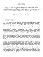
Figure 1: Simulated coastal point source pollution by an aerobically
degrading organic contaminant.
where
c
i
is the molar concentration of the (uncomplexed) aqueous
component,
n
s
is the number of species in dissolved form that have
complexed with the aqueous component,
s
j
Y
is the stoichiometric coefficient
of the aqueous component in the
j
th
complexed species, and s
j
is the molar
concentration of the
j
th
complexed species. As in PHT3D, the (local) redox-
state, pe, is modeled by transporting chemicals/components in different
redox states separately, while the pH is modeled from the (local) charge

balance.
Coupling of PHREEQC-2 with SEAWAT is achieved through a
sequential operator splitting technique [Yeh and Tripathi, 1989; Barry
et al.,
2002], similar to the technique used for the PHT3D model, which couples
PHREEQC-2 with MT3DMS. The splitting scheme used to solve the
advection-dispersion-reaction equation (Eq. (1)) for a user-defined time step
length consists of two steps. In the first step the advection and dispersion
term of mobile species/components is solved with SEAWAT for the time
step length
t∆ . In the subsequent step the reaction term r
reac
in Eq. (1) is
solved through grid-cell wise batch-type PHREEQC-2 reaction calculations.
This step accounts for the concentration changes that have occurred during
t∆ as a result of reactive processes. The reaction term r
reac
in Eq. (1)
corresponds to the computed concentration differences from before
(PHREEQC-2 input concentrations) and after the reaction step (PHREEQC-2
output concentrations).
Figure 1 illustrates the results from one of the initial (simple) multi-
species test simulations of coastal point-source pollution by an organic
contaminant. The plume is degraded aerobically, i.e., the degradation
reaction creates an oxygen-depleted zone in an aquifer containing
groundwater of variable density.
© 2004 by CRC Press LLC
Coastal Aquifer Management
54
2.3 Integrated Surface-Water and Groundwater Modeling with

SWIFT2D and SEAWAT
2.3.1 Code Description
To simulate the coastal hydrology of the southern Everglades of
Florida, which is characterized by shallow overland flow and subsurface
groundwater flow, SEAWAT was coupled with the hydrodynamic estuary
model, SWIFT2D (Surface-Water Integrated Flow and Transport in 2-
Dimensions) [Langevin
et al, 2002; Langevin et al., 2003; Swain et al.,
2003]. SWIFT2D solves the full dynamic wave equations, including density
effects, and can also represent transport of multiple constituents, such as the
dissolved species in seawater. The SWIFT2D code was originally developed
in the Netherlands [Leendertse, 1987], and was later modified by the U.S.
Geological Survey to represent overland flow in wetlands by including
spatially varying rainfall, evapotranspiration, and wind sheltering
coefficients [Swain
et al., 2003].
The coupling of SWIFT2D and SEAWAT is accomplished by
including the programs as subroutines of a main program called FTLOADDS
(Flow and Transport in a Linked Overland-Aquifer Density Dependent
System). FTLOADDS uses a mass conservative approach to couple the
surface water and groundwater systems, and computes leakage between the
wetland and the aquifer using a variable-density form of Darcy’s Law written
in terms of equivalent freshwater head. The leakage representation also
includes associated solute transfer, based on leakage rates, flow direction,
and solute concentrations in the wetland and aquifer.
Coupling between SWIFT2D and SEAWAT occurs at intervals
equal to the stress period length in the groundwater model. For each stress
period, which is one day in the current Everglades application, SWIFT2D is
called first, using short timesteps, such as 15 minutes, to complete the entire
groundwater model stress period. Within the SWIFT2D subroutine, leakage

is calculated as a function of the surface water stage and the groundwater
head from the end of the previous stress period. The total leakage volumes
(for each cell) are summed for the stress period by accumulating the product
of the leakage rate and the length of the surface water timestep. After
SWIFT2D completes the stress period, the total leakage volumes are applied
on a cell-by-cell basis to SEAWAT as it runs for the same stress period to
calculate groundwater heads and solute concentrations.
FTLOADDS also accounts for the net solute flux between surface
water and groundwater. When the leakage volume is computed for a surface-
water timestep, the solute flux is computed based on flow direction. If the
flow is upward from the aquifer into the wetland, the solute flux is calculated

© 2004 by CRC Press LLC
MODFLOW-Based Tools
55

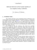
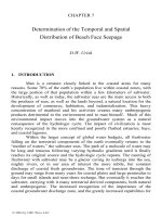
Figure 2: Map of southern Florida showing SICS model domain and
simulated values of average daily leakage between surface water and
groundwater.
by multiplying leakage volume and groundwater salinity. The calculated
solute mass is then added to the surface-water cell in the SWIFT2D transport
subroutine. If flow is downward from the wetland into the aquifer, the solute
mass flux is calculated as the product of leakage volume and surface-water
salinity. The total solute mass flux is summed for the surface-water timesteps
and divided by the total leakage volume. This gives an equivalent salinity
concentration for the total leakage over the stress period. Whichever
direction of the leakage, the computed equivalent salinity is used in
SEAWAT as the concentration of the water added or removed from the
aquifer as leakage.
2.3.2 Application to the Southern Everglades of Florida

As part of the Comprehensive Everglades Restoration Plan, the U.S.
Geological Survey has applied the FTLOADDS model to the Taylor Slough
area in the southern Everglades of Florida (Figure 2) [Langevin
et al., 2002].
© 2004 by CRC Press LLC
Coastal Aquifer Management
56
The finite-difference grid consists of 148 columns and 98 rows. Each cell is
square with 304.8 m per side. The three-dimensional grid has 10 layers
(each 3.2 m thick) and extends from land surface to a depth of 32 m. The
integrated model simulates flow and transport from 1995 through 1999.
The integrated surface water and groundwater model was calibrated
by adjusting model input parameters until simulated values of stage, salinity,
and flow matched with observed values at the wetland and Florida Bay
monitoring sites. Daily leakage rates between surface water and groundwater
are produced as part of the model output for each cell. These daily leakage
rates were averaged over the 5-year simulation period to illustrate the spatial
variability in surface water/groundwater interaction (Figure 2). These
leakage rates do not include recharge or evapotranspiration directly to or
from the water table. The model suggests an alternating pattern of
downward and upward leakage from north to south (Figure 2). To the north,
most leakage is downward into the aquifer, except near the Royal Palm
Ranger station where upward flow occurs near Old Ingraham Highway.
Further south, a large area of upward leakage exists. This area of upward
leakage roughly corresponds with the location of the freshwater/saltwater
interface in the aquifer. In this area, groundwater flowing toward the south
moves upward where it meets groundwater with higher salinity. To the
south, leakage is downward into the aquifer. The Buttonwood Embankment,
which is a narrow ridge along the Florida Bay coastline, separates the inland
wetlands from Florida Bay. The embankment impedes surface water flowing

south and increases wetland stage levels to elevations slightly higher than
stage levels in Florida Bay. South of the Buttonwood Embankment,
groundwater discharges upward into the coastal embayments of Florida Bay.
This upward leakage in the model is caused by the higher water levels on the
north side of the embankment. These model results suggest that surface
water and groundwater interactions are an important component of the water
budget for the Taylor Slough area.
3. MOCDENS3D
G.H.P. Oude Essink
3.1 Program Description
The computer code MOCDENS3D [Oude Essink, 1998, 2001] can
simulate groundwater flow and coupled solute transport in porous media.
The code is based on the United States Geological Survey public domain
three-dimensional finite difference computer code MOC3D [Konikow
et al.,
1996]. Density differences in groundwater are taken into account in the
mathematical formulation. So-called freshwater heads and buoyancy term are
© 2004 by CRC Press LLC
MODFLOW-Based Tools
57
introduced. As a result, it is possible to simulate non-stationary flow of fresh,
brackish, and saline groundwater in coastal aquifers. More detail of the code
is described in Oude Essink [1999]. Note that MOCDENS3D is similar to
SEAWAT: the first uses MOC3D for solute transport, whereas the latter
applies MT3DMS [Zheng and Wang, 1999].
3.2 Effect of Sea Level Rise and Land Subsidence in a Dutch Coastal
Aquifer
3.2.1 Introduction to the Dutch Situation
Saltwater intrusion is threatening coastal groundwater systems in the
Netherlands. At the root of the problem are both natural processes and

anthropogenic activities that have been going on for centuries. Autonomous
events, land subsidence, and sea level rise all influence the distribution of
fresh, brackish, and saline groundwater in Dutch coastal aquifers.
The greatest land subsidence is occurring in the peaty and clayey
regions in the west and north of the Netherlands and emanates from two,
human-driven processes. The first—soil drainage—is a slow and continuous
process that started about a thousand years ago when the Dutch began to
drain their swampy land. The second—land reclamation—causes a relatively
abrupt change in the surface level. In particular, it was the reclamation of the
deep lakes during the past centuries that caused the strong flow of saline
groundwater from the sea to the coastal aquifers. These so-called
deep
polders
are currently experiencing upward seepage flow.
An example of a Dutch coastal aquifer will show that on the long
term, the effects of sea level rise and land subsidence—in terms of the
amount of seepage, average salt content, and salt load—can be considerable
[Oude Essink and Schaars, 2003].
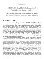
3.2.2 Model of the Groundwater System of Rijnland Water Board
The Rijnland Water Board has a surface area of about 1,100 km
2

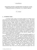
(Figure 3a) and accommodates some 1.3 million people. Since the 12th
century, the water board manages water quantity and water quality aspects in
the area. Sand dunes are present at the western side of the water board
(Figure 3b). Three major drinking water companies are active in the dunes:
DZH (Drinking Water Company Zuid-Holland), GWA (Amsterdam
Waterworks), and PWN (Water Company Noord-Holland).
Phreatic water levels in the dune areas can go up to more than 7
meters above mean sea level. At the inland side of the dune area, some large

low-lying polder areas with controlled water levels occur (Figure 4a). The
lowest phreatic water levels in the water board itself can be found northwest
of the city Gouda (down to nearly −7 m N.A.P.) and in the Haarlemmermeer

© 2004 by CRC Press LLC
Coastal Aquifer Management
58

Figure 3: (a) Map of The Netherlands: position of the Rijnland Water Board
and ground surface of the Netherlands; (b) Map of the Rijnland Water Board:
position of some polder areas and the sand-dune areas of the drinking water
companies DZH, GWA, and PWN. The Haarlemmermeer polder is also a
part of the water board.
polder, where the airport Schiphol is located, with levels as low as −6.5 m
N.A.P. Before the middle of the 19th century, a lake covered the
Haarlemmermeer polder area. Due to flooding threats in the neighboring
cities, this lake was reclaimed during the years 1840–1852 which caused a
relative abrupt change in heads. Subsequently, a completely different
groundwater flow regime was created regionally. In addition, the polder
Groot-Mijdrecht, situated outside the water board, is also mentioned here.
Though the surface area of this polder is not large, the phreatic water level is
low (less than −6.5 m N.A.P.) and the Holocene aquitard on top of the
groundwater system is very thin. Seepage in this area is very large (more
than 5 mm/day) and groundwater from a large region around it is flowing to
the polder at a rapid pace. Some large groundwater extractions from the
lower aquifer system are taking place, up to 20 million m
3
/yr at Hoogovens
near IJmuiden.
The groundwater system consists of a three-dimensional grid of

52.25 km by 60.25 km (~3,150 km
2
) by 190 m depth and is divided into a
large number of elements. Each element is 250 m by 250 m in horizontal
plane. In vertical direction the thickness of the elements varies from 5 m for
the 10 upper layers to 10 m for the deepest 14 layers (Figure 4b). The grid

© 2004 by CRC Press LLC
MODFLOW-Based Tools
59


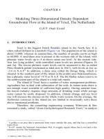
Figure 4: (a) Phreatic water levels or polder levels in the area (note that in
the sand-dune areas, no polder levels are given); (b) Simplified subsoil
composition of the bottom of the water board of Rijnland and hydraulic
conductivity values.
contains 1,208,856 active elements:
n
x
= 209, n
y
= 241, n
z
= 24, where n
i

denotes the number of elements in the
i direction. Each element contains
initially eight particles, which gives in total 9.6 million particles to solve the
advection term of the solute transport equation. The flow time step ∆

t to
recalculate the groundwater flow equation is 1 year. The convergence
criterion for the groundwater flow equation (freshwater head) is equal to 10
−4

m.
Data has been retrieved from NAGROM (The National Groundwater
Model of The Netherlands). Figure 4b shows the composition of the
groundwater system into three permeable aquifers, intersected by an aquitard
in the upper part of the system and an aquitard of clayey and peat composite
between −70 and −80 m N.A.P. For each subsystem, the interval of the
horizontal hydraulic conductivity
k
h
is given in the figure. The anisotropy
ratio
k
z
/k
x
is assumed to be 0.1 for all layers. The effective porosity n
e
is a bit
© 2004 by CRC Press LLC
Coastal Aquifer Management
60
low: 25%. The longitudinal dispersivity
α
L
is set equal to 1 m, while the ratio

of transversal to longitudinal dispersivity is 0.1.
The bottom of the system is a no-flow boundary. Hydrostatic
conditions occur at the four sides of the model. At the top of the system, the
natural groundwater recharge in the sand-dune area varies from 0.94 to 1.14
mm/day. The water level at the sea is set to 0.0 m N.A.P. for the year 2000
AD. The general head boundary levels in the polder area are equal to the
phreatic water level in the considered polder units, varying from +2.0 m near
IJmuiden to −7.0 m N.A.P. northwest of Gouda.
At the initial situation (2000 AD), the hydrogeologic system contains
saline, brackish as well as fresh groundwater. On the average, the salinity
increases with depth, whereas freshwater lenses exist at the sand-dune areas
at the western part of the water board, up to −90 m N.A.P. Freshwater from
the sand dunes flows both to the sea and to the adjacent low-lying polder
areas. The chloride concentration of the upper layers is already quite high in
some low-lying polder areas such as the Haarlemmermeer polder and the
polder Groot-Mijdrecht. The volumetric concentration expansion gradient
β
C

is 1.34x10
−6
l/mg Cl
-
. Saline groundwater in the lower layers does not
exceed 18,630 mg Cl
-
/l. The corresponding density of that saline
groundwater equals 1,025 kg/m
3
.

Calibration was focused on freshwater heads in the hydrogeologic
system, and to some extent on seepage and salt load values in the
Haarlemmermeer polder and the polder Groot-Mijdrecht. Calibration data
has been derived from the water board itself, the NAGROM database, ICW
(1976), and the DINO database of Netherlands Institute of Applied
Geosciences (TNO-NITG). The model was calibrated by comparing 1632
measured and computed freshwater heads, and for seepage and salt load
values of some polders. Note that the measured heads are corrected for
density differences. The mean error between measured and computed
freshwater heads is −0.16 m, the mean absolute error 0.61 m, and the
standard deviation 0.79 m.
3.2.3 Sea Level Rise and Land Subsidence
It is expected that climate change causes a rise in mean sea level and
a change in natural groundwater recharge. As exact figures are not known
yet, an average impact scenario is considered here by taking into account the
most likely future developments in this area:
• According to the Intergovernmental Panel of Climate Change [IPCC,
2001], a sea level rise of 0.48 m is to be expected for the year 2100
(relative to 1990), with an uncertainty range from 0.09 to 0.88 m.
Based on these figures, a sea level rise of 50 cm per century will be
© 2004 by CRC Press LLC
MODFLOW-Based Tools
61
implemented at the North Sea, in steps of 0.005 m per time step of 1
year, from 2000 AD on.
• An instantaneous increase of natural groundwater recharge of 3% at all
sand-dune areas in 2000 AD.
• Oxidation of peat, compaction and shrinkage of clay, and groundwater
recovery are causing land subsidence, especially in the peat areas of
the water board. The following values are inserted: a land subsidence

of –0.010 m per year for the peat areas; no subsidence for the sand-
dune areas; and –0.003 m per year for the rest of the land surface
(respectively 25, 9, and 66% of the land surface in the entire modeled
area).
• A reduction of groundwater extraction in the sand-dune areas GWA
(–1.3 million m
3
/yr) and PWN (–4.5 million m
3
/yr).
The total simulation time is 200 years.
3.2.4 Discussion of Results
The overall picture is that the groundwater system will contain more
saline groundwater these coming centuries. The numerical model supports
the theory that the present situation is not in equilibrium from a salinity point
of view. Figure 5 shows the chloride distribution at –2.5 and –7.5 m N.A.P.
for the years 2000 and 2200 AD. Salinization is going on, especially in the
areas close to the coastline. Though the differences look small due to the fact
that groundwater flow and subsequently solute transport are slow processes,
changes in seepage and salt load at the top aquifer system are pretty
significant (Figure 6). The combination of autonomous development
(reclamation of the deep lakes in the past), sea level rise, and land subsidence
will intensify the salinization process: partly due to an increase of seepage
values (+6% in 2050 and +12% in 2200, relative to now) but mainly due to
the increase in salinity of the top aquifer system. As a result, the overall salt
load in the water board is estimated to increase +38% in 2050 and even
+79% in 2200, relative to now. The more rapid increase in salt load is caused
by an increased salinization of the upper aquifers.
3.2.5 Conclusions
A model of the variable density groundwater flow system of the

Rijnland Water Board is constructed to quantify the effect of past
anthropogenic activities, climate change (rise in sea level and an increase in
natural groundwater recharge in the sand-dune areas), and land subsidence in
large parts of the area. The code MOCDENS3D is used to simulate density
dependent groundwater flow under influence of the above mentioned
stresses. Numerical computations indicate that a serious saltwater intrusion

© 2004 by CRC Press LLC
Coastal Aquifer Management
62


Figure 5: Chloride concentration at –2.5 and –47.5 m N.A.P. for the years
2000 and 2200 AD. Sea level rise and land subsidence is considered.
can be expected during the coming decennia, mainly because a large part of
the Rijnland Water Board is lying below mean sea level. The combined
effect for 2050 AD will be: a 6% increase of seepage and a 38% increase of
salt load in the Rijnland Water Board. The increase especially in salt load
will definitely affect surface water management aspects at the water board.

© 2004 by CRC Press LLC
MODFLOW-Based Tools
63

Figure 6: Seepage (in m
3
/day) and salt load (in ton Cl
-
/year) through the
second model layer at –10 m N.A.P., summarized for the entire Rijnland

Water Board, as a function of 200 years.
4. MODHMS
S. Panday, W. Jones, M. Beach, M. Barcelo
4.1 Program Description
4.1.1 Description
MODHMS [HydroGeoLogic, 2002] is a comprehensive hydrologic
modeling system that extends MODFLOW to include the unsaturated zone,
the overland flow domain, and channel/surface-water features. Contaminant
transport routines are also incorporated for fate and transport calculations in
single or dual porosity systems. Density coupling of the flow-field with
concentrations of some or all species provides comprehensive analysis
capabilities for complex coastal issues.
4.1.2 Physical Concepts and Model Features
MODFLOW's capabilities are expanded by MODHMS to solve the
Richards equation for three-dimensional saturated-unsaturated subsurface
flow, coupled with the diffusive wave equations for two-dimensional
overland and one-dimensional channel flow (including effects of scale, pond
storage, routing, and hydraulic structures). The primitive form of the
transport equation for single or multiple species is also solved, with optional
dual porosity considerations for the subsurface. Nonlinear adsorption and
linear decay processes are incorporated, with provisions to accommodate
user-supplied, complex reaction modules. Multi-phase transport occurs with
equilibrium partitioning considerations and diffusion/storage/decay in the
inactive (air) phase. Non-isothermal conditions may be simulated by
allocating the temperature variable as the first species of solution. Density
© 2004 by CRC Press LLC
Coastal Aquifer Management
64
coupling (in surface and subsurface regimes) of flow with transport of some
or all contaminant species is achieved via a linear density relationship with

concentration (adjustment of viscosity and density for the conductance term
may also be optionally applied). Fluid pressure is therefore affected by
species concentration, and the advection and dispersion terms are affected by
the resultant volumetric fluid fluxes. Various combinations of the above
simulation capabilities may be used for optimal solution to a given problem.
In addition to MODFLOW’s stress packages, MODHMS includes
fracture-wells to handle multi-layer pumping and prevent overpumping; an
unconfined recharge seepage-face package (for subsurface simulations only)
for ponding and hill slope seepage issues; and a comprehensive
evapotranspiration (ET) package that accounts for climatic conditions.
Transport boundaries include mass fluxes at inflow nodes and prescribed
concentrations anywhere in the domain. For density-dependent cases, the
flow condition is optionally checked at every iteration or time-step at a
constant head node, before applying a prescribed concentration condition.
4.1.3 Computational Aspects
The three-dimensional finite-difference grid of MODFLOW is used
for subsurface discretization, with a corresponding two-dimensional grid for
the overland domain, and a finite-volume discretization for the
channel/surface-water body domain. Alternatively, an orthogonal curvilinear
grid may be used for the overland and subsurface regimes.
Surface/subsurface interactions are expressed fully implicitly, or via
iterative/linked options. Newton-Raphson linearization may be used for the
unsaturated or unconfined flow equations, and pseudo-soil functions (that are
more robust for wetting/drying situations) may be used for unconfined
systems where unsaturated effects are neglected. The transport equations are
solved using mass conserved schemes with Total Variation Diminishing
(TVD), upstream or midpoint spatial weighting, and implicit or Crank-
Nicolson temporal weighting options. For density-dependent simulations, the
flow equation is solved in terms of equivalent freshwater heads, and the
density correction is applied via Picard iteration between the flow and

transport equations. Adaptive time-stepping and under-relaxation formulas
are based on all system non-linearities, for optimal speed and robustness.
Solution options are provided for various combinations of transient and
steady-state flow and transport analysis.
© 2004 by CRC Press LLC
MODFLOW-Based Tools
65
#
Y
#
Y
#
Y
#
Y
#
Y
Tampa
Clearwater
St. Petersburg
MANATEE
HILLSBOROUGH
SARASOTA
CHARLOTTE
PINELLAS
Gulf of Mexic o
T
a
m
p

a

B
a
y
0
.
1
0
.
9
0
.
5
0.1
0.5
0.5
0.1
0.5
0.5
0
.
0
5
Bradenton
Saraso ta
Surface Drainage
County Boundary
Legend
Model Domain Inactive Area

Relative Chloride Concentration Contour
0.05
1.0 = 19,000 mg/l
05
Miles
N
Locator Map

Figure 7: Location of study area and simulated chloride concentrations.
4.2 Case History
4.2.1 Site Location and Project Objectives
The study area lies in the southern portion of the Southwest Florida
Water Management District (SWFWMD). The model domain includes all or
portions of Pinellas, Hillsborough, Manatee, and Sarasota Counties and
extends into the Gulf of Mexico covering approximately 60 miles by 100
miles (Figure 7). Management of saltwater intrusion due to significantly
increased groundwater withdrawals was investigated using a density-
dependent MODHMS model. Boundary conditions and model parameters
were derived from a larger, regional MODFLOW model developed by the
SWFWMD and referred to as the Southern District (SD) model. The local
© 2004 by CRC Press LLC
Coastal Aquifer Management
66
model was calibrated to available chloride and water level information from
pre-development to current conditions. A steady-state pre-development
calibration provided assumed hydrostatic equilibrium behavior of the
flow/transport system under long-term average recharge conditions, and was
followed by a post-development transient simulation using pumping
estimates throughout the study area, from 1900 to 2000. The calibrated
model was used to predict the impact of several potential water management

scenarios from current conditions to 2050. Results of this analysis assisted in
the development of a water level index that will aid in long-term
management of groundwater resources. The CD accompanying this book
contains the detailed report of this study [HydroGeoLogic, 2002].
4.2.2 Climate and Hydrogeologic Setting
The site location is humid and subtropical, characterized by warm
wet summers and mild dry winters. Long-term rainfall averages 52 in/yr, and
mean evapotranspiration is 39 in/yr. The underlying aquifers include the
Surficial Aquifer System (SAS), the Intermediate Aquifer System (IAS), and
the Floridan Aquifer System (FAS), each of which consists of permeable
layers separated by lower permeability semi-confining units. The FAS is
subdivided into major units comprising the Upper Floridan Aquifer (UFA),
the Middle Confining Unit (MCU), and the Lower Floridan Aquifer (LFA),
which is highly saline in this region and not a source of potable water. The
UFA is the principal source of water in the region and is further subdivided
into the Suwannee Limestone, the Ocala Limestone, and the Avon Park
Formation, which consists of a main water-bearing zone overlying relatively
lower-conductivity units. The MCU contains evaporites that are of extremely
low conductivity and forms the bottom of the modeled system.
4.2.3 Conceptual Model and Calibration
The density-dependent saltwater intrusion model was developed
from the SD model using telescoping mesh refinement, thereby maintaining
the hydrostratigraphy, hydrogeologic properties, and imposed stresses of the
regional model. Hydrogeologic units were further sub-divided vertically in
the numerical grid of the local model to provide resolution for saltwater
intrusion considerations. Only the FAS was considered for this study,
therefore, recharge/discharge from the overlying IAS was obtained from
regional flow model results and applied as a general head boundary across
the overlying confining unit. The saltwater model domain included the
Suwannee Limestone underlain by the Ocala limestone, the Avon Park

Formation and the low conductivity Evaporite Zone of the MCU. Chloride
and head conditions were prescribed underneath, for provision of upward

© 2004 by CRC Press LLC
MODFLOW-Based Tools
67
Chloride Concentration (mg/L)
Elevation (ft)
0 5000 10000 15000
-1400
-1200
-1000
-800
-600
-400
-200
0
Simulated Chl or i de Concentrations
Observed Chloride Concentrations from
ROMP Well TR 8-1

Figure 8: Comparison of observed and simulated chloride concentrations.
movement and upconing effects from deeper regions. Hydraulic conductivity
values of the various formations were derived from the SD model
transmissivity and leakance fields, and landward boundary conditions for
each model run were obtained from parallel simulations using the SD model.
Vertical anisotropies, dispersivities, and saltwater boundaries were obtained
from field estimates or treated as calibration parameters. Conductivity fields
were also adjusted slightly.
The model was first calibrated to steady-state environmental heads,

and depth-to-chlorides (for 250, 500, and 1000 ppm levels) estimated for pre-
development conditions (early 1900s), with further calibration for transients
till the year 2000 (Figure 8). Calibration measures include collective
statistics as well as temporal and depth-dependent heads and chloride
concentrations obtained from individual wells. The model was used to
predict the effects of different stresses within the SWUCA (400, 600, 800,
and 1000 MGD) for the next 50 years, to determine relations between
pumping, flow levels, and long-term saltwater intrusion in the FAS.
4.2.4 Model Calibration Results
The MODHMS model was able to accurately simulate hydraulic
heads and chloride concentrations within the study area. The calibration to
environmental heads was good, and the model adequately represented

© 2004 by CRC Press LLC
Coastal Aquifer Management
68
horizontal axis
vertical axis
density density
A
A' a
b
c
fresh w ater
brackish 1
brackish 2
salt w ater

Figure 9: (a) Conceptual model with three surfaces, (b) density distribution
of stratified flow, (c) density distribution of variable density flow.

depth-dependent chloride concentrations (Figure 8) and chloride movement
from pre- to post-development conditions (Figure 7). Calibration results are
also in agreement with qualitative historical data and with previous modeling
efforts.
5. THE SWI PACKAGE
M. Bakker
The Sea Water Intrusion (SWI) package is intended for modeling
regional seawater intrusion with MODFLOW. The package may be used to
simulate the three-dimensional evolution of the salinity distribution, taking
density effects into account explicitly. The main advantage of the SWI
package is that each aquifer can be modeled with a single layer of cells,
without requiring vertical discretization of an aquifer. An existing
MODFLOW model of a coastal aquifer can be modified to simulate seawater
intrusion with the SWI package through the addition of one input file. The
SWI package can simulate interface flow, stratified flow, and continuously
varying density flow.
5.1 Theory
The basic idea behind the SWI package is that the groundwater in
each aquifer is discretized vertically into a number of zones bounded by
curved surfaces. A schematic vertical cross-section of an aquifer is shown in
Figure 9a; the thick lines represent the surfaces. The elevation of each
surface is a unique function of the horizontal coordinates. The SWI package
has two options. For the
stratified flow option, water has a constant density
between surfaces and the surfaces represent interfaces; the density is
discontinuous across a surface (Figure 9b). For the
variable density flow
© 2004 by CRC Press LLC
MODFLOW-Based Tools
69

option, the surfaces represent iso-surfaces of the density; the density varies
linearly in the vertical direction between surfaces and is continuous across a
surface (Figure 9c).
Four main approximations are made:
• The Dupuit approximation is adopted and is interpreted to mean that
the resistance to flow in the vertical direction is neglected. The Dupuit
approximation is accurate for many practical problems of interface
flow, even when the slope of the interface is relatively steep (up to
45°), and for variable density flow [Strack and Bakker, 1995]. The
vertical pressure distribution is hydrostatic in each aquifer, but this
does not mean that there is no vertical flow; the vertical component of
flow is computed from three-dimensional continuity of flow.
• The mass balance equation is replaced by the continuity of flow
equation in the computation of the flow field (the Boussinesq-
Oberbeck approximation); density effects are taken into account
through Darcy’s law.
• Effects of dispersion and diffusion are not taken into account.
• Inversion is not allowed. Inversion means that saltier (heavier) water is
present above fresher (lighter) water, often resulting in the vertical
growth of fingers. The SWI package is intended for the modeling of
regional seawater intrusion, which is generally on a scale well beyond
the size of the fingers.
Dependent variables in the formulation are the freshwater head at
the top of each aquifer and the elevations of the surfaces in each aquifer, and
the vertically integrated fluxes. Application of continuity of flow in each
aquifer results in a system of differential equations for the freshwater head
that is identical in form to the differential equations for single-density flow,
but with an additional pseudo-source term, representing the density effects,
on the right-hand side (RHS). Hence, MODFLOW can be used to compute
the distribution of the freshwater head by addition of this pseudo-source term

to the RHS. The differential equations that govern the movement of the
surfaces have the same form as the equations for the head, but with different
values for the transmissivities and pseudo-source term. Since the form is the
same, the solution engines of MODFLOW can again be applied to solve the
system for every timestep. A simple tip/toe tracking algorithm is applied to
keep track of the horizontal positions of the surfaces. Details of the theory
implemented in the SWI package may be found in Bakker [2003].

© 2004 by CRC Press LLC
Coastal Aquifer Management
70

0 500 1000 1500 2000 2500
0
500
1000
1500
2000
2500
East-West
South-North
well
-19
shore
0 500 1000 1500 2000 2500
East-West
-26
-34
-36
-40

shore in
top aquifer

Figure 10: Contours of interface elevation below an island with a well in the
top aquifer after 40 years of pumping: top aquifer (left) and bottom aquifer
(right).
5.2 Example Application
The SWI package is implemented in MODFLOW2000. Only one additional
input file is needed to simulate seawater intrusion. The input file consists of
the elevations of the surfaces in each aquifer, the density between the
surfaces, whether flow should be treated as stratified or variable density, and
some tip/toe tracking parameters. MODFLOW/SWI may then be used to
compute the positions of the surfaces at the requested times. Details of
application of the SWI package may be found in the manual [Bakker and
Schaars, 2003]; an executable, a manual, and the source code are available
for free download from the author’s web page.
2

One of the major benefits of the SWI package is that it can simulate
interface flow, stratified flow, and variable density flow efficiently, even in
the same model. Especially when little data is available, it is useful to
determine the steady-state position of the interface. This position may
already be sufficient to solve the posed problem, or may be used as a starting
point for additional transient simulations. When a significant brackish zone is
present, the interface may be replaced by one or more brackish zones, either
of constant density or variable density. One aquifer may have an interface,
while another may have a brackish zone, as will be demonstrated below.


2

© 2004 by CRC Press LLC
MODFLOW-Based Tools
71


0 500 1000 1500 2000 2500
-50
-40
-30
-20
-10
0
East-West
well screen
interface in
top aquifer
leaky layer


Figure 11: Upconing of brackish zone along east-west cross-section through
well: 20 years (dashed), 40 years (solid), interface after 40 years (bold).
Consider seawater intrusion below the hypothetical five-sided island shown
in Figure 10. The top aquifer extends from 0 to –20 m, and has a
transmissivity of 100 m
2
/d; the bottom aquifer extends from –25 to –55 m,
and has a transmissivity of 150 m
2
/d. The leakance (V

cont
) of the leaky layer
is 0.002 d
-1
. The island is surrounded by the ocean, with a fixed level of 0 m;
the vertical leakance of the bottom of the ocean, representing the vertical
resistance to outflow into the ocean, is 0.1 d
–1
. Recharge on the island is 0.5
mm/d and is specified with the RCH package. The effective porosity of both
aquifers is 0.2. The freshwater heads are computed assuming consecutive
steady-state conditions, as the heads will react much quicker than the
position of the interface; heads can be treated as transient as well, but
modeling them as consecutive steady-states has little influence on the results
and allows for the specification of much larger timesteps.
The island is discretized into cells of 25 by 25 meters; the grid is
extended at least 350 m into the ocean in all directions. The ocean cannot be
modeled with GHB cells, as all sinks and sources in the SWI package are
treated as consisting of freshwater. The ocean is modeled with an additional
layer on top of the model, consisting of inactive cells wherever the island
sticks out of the ocean, and fixed head cells elsewhere. Surfaces or interfaces
will be specified at the top of the additional layer, such that all water in the
additional layer is salt.
As a first step in the modeling process, flow is treated as interface
flow. The saltwater has a density of 1,025 kg/m
3
. The maximum slope of the
interface is specified as 0.03, and the other two tip/toe tracking parameters
are specified according to the guidelines in the SWI manual. The steady-
state position of the interface is approached after 80 steps of 250 days,

© 2004 by CRC Press LLC
Coastal Aquifer Management
72
starting from a rough first guess. The freshwater zone in the bottom aquifer
is over 18 m thick in the middle of the island. The steady-state position is
used as a starting point for further modeling. A well is started in the top
aquifer and has a discharge of 200 m
3
/d (about 10% of total recharge on the
island). Contours of the elevation of the interface after 40 timesteps of 1 year
are shown in Figure 10. The well has little effect on the position of the
interface in the top aquifer, but there is an upconing of 8 m below the well in
the bottom aquifer.
As it is crucial for the saltwater to remain in the bottom aquifer and
not reach the leaky layer below the well, modeling is continued by replacing
the interface in the lower aquifer with a brackish zone, initially extending 5
m above the steady-state position of the interface. The brackish water has a
constant density of 1012.5 kg/m
3
. The position of the brackish zone along an
east-west cross-section through the well is shown after 20 years (dashed) and
40 years (solid) of pumping in Figure 11; results of the interface simulation
after 40 years of pumping are also shown in the figure (thick line). It is
concluded that the top of a 5 m thick brackish zone will reach the bottom of
the leaky layer after 40 years.
6. SUMMARY
This chapter presents four MODFLOW-based codes for simulation
of variable-density groundwater flow. An example application was presented
for each code to demonstrate the simulation capabilities. Additional
information for each code can be found on the accompanying CD of this

book.
REFERENCES
Bakker, M., “A Dupuit formulation for modeling seawater intrusion in
regional aquifer systems,”
Water Resources Research, in print, 2003.
Bakker, M. and Schaars, F., “The Sea Water Intrusion (SWI) package
manual, version 0.2,”
2003.
Barry, D.A., Prommer, H., Miller, C.T., Engesgaard, P., and Zheng, C.,
“Modelling the fate of oxidisable organic contaminants in
groundwater,”
Adv. Water Resources, 25, 899–937, 2002.
Christensen, F.D., Basberg, L., and Engesgaard, P., “Modeling transport and
biogeochemical processes in dense landfill leachate plumes,” In:
Computational Methods in Water Resources, Proceedings of the
XIVth International Conference, Delft, Netherlands, June 23–28,
2002.
© 2004 by CRC Press LLC
MODFLOW-Based Tools
73
Christensen, F.D., Engesgaard, P., and Kipp, K.L., “A reactive transport
investigation of seawater intrusion experiment in a shallow aquifer,
Skansehage, Denmark,” Proceedings of the First International
Conference on Saltwater Intrusion and Coastal Aquifers, Essaouira,
Morocco, April 23–25, 2001.
Clement, T.P., “A modular computer code for simulating reactive
multispecies transport in 3-dimensional groundwater systems,”
Technical report PNNL-SA-11720, Pacific Northwest National
Laboratory, Richland, WA, 1997.
Guo, W. and Bennett, G.D., “SEAWAT version 1.1: A computer program

for simulations of groundwater flow of variable density,” Missimer
International, Inc., Fort Myers, FL, 1998.
Guo, W. and Langevin, C.D., “User’s guide to SEAWAT: A computer
program for simulation of three-dimensional variable-density
ground-water flow,” U.S. Geological Survey Open-File Report 01-
434, 79 p., 2002.
Harbaugh, A.W. and McDonald, M.G., “User's documentation for
MODFLOW-96, an update to the U.S. Geological Survey modular
finite-difference ground-water flow model,” U.S. Geological Survey
Open-File Report 96-0485, 56 p., 1996.
Harbaugh, A.W., Banta, E.R., Hill, M.C., and McDonald, M.G.,
“MODFLOW-2000, the U.S. Geological Survey modular ground-
water model—user guide to modularization concepts and the
ground-water flow process,” U.S. Geological Survey Open-File
Report 00-92, 121 p., 2000.
Hill, M.C., Poeter, E., Zheng, C., and Doherty, J., “MODFLOW2001 and
other modeling odysseys,”
Ground Water, 41, 113, 2003.
Hsieh, P.A. and Winston, R.B., “User’s guide to Model Viewer, a program
for three-dimensional visualization of ground-water model results,”
U.S. Geological Survey Open-File Report 02-106, 18 p., 2002.
HydroGeoLogic, Inc., “MODHMS—MODFLOW-based Hydrologic
Modeling System: Documentation and User's Guide,” 2002.
HydroGeoLogic, Inc., “Three-dimensional density-dependent flow and
transport modeling of saltwater intrusion in the Southern Water Use
Caution Area,” Prepared for the Southwest Florida Water
Management District, June 2002.
ICW, “Hydrology and water quality of the central part of the western
Netherlands,” (in Dutch), ICW Regional Studies 9, Institute for Land
and Water Management Research, Wageningen: 101 pp., 1976.

IPCC, Intergovernmental Panel on Climate Change. Climate “Change 2001:
The Scientific Basis,” 2001.
© 2004 by CRC Press LLC