COASTAL AQUIFER MANAGEMENT: monitoring, modeling, and case studies - Chapter 10 docx

CHAPTER 10
Uncertainty Analysis of Seawater Intrusion and
Implications for Radionuclide Transport at Amchitka
Island’s Underground Nuclear Tests
A. Hassan, J. Chapman, K. Pohlmann
1. INTRODUCTION
All studies of subsurface processes face the challenge presented by
limited observations of the environment of interest. By its very nature, the
detailed characteristics of the subsurface are hidden and data collection
efforts are generally hindered by technical and financial constraints. The
result is that uncertainty is a factor in all groundwater studies. Seawater
intrusion environments present both special opportunities and special
challenges for incorporating uncertainty into numerical simulations of
groundwater flow and contaminant transport. Opportunities come from the
constraints that the seawater–freshwater system provides; challenges come
from the numerically intensive solutions demanded by simultaneous solution
of the energy and mass transport equations.
The impact of uncertainty in the analysis of contaminant transport in
coastal aquifers is an important aspect of evaluating radionuclide transport
from three underground nuclear tests conducted by the U.S. on Amchitka
Island, Alaska. Testing was conducted in the 1960s and very early 1970s on
the Aleutian island to characterize the seismic signals from underground tests
in active tectonic regimes, and to avoid proximity to high-rise buildings and
resulting ground motion problems. As the U.S. Department of Energy
focused on environmental management of nuclear sites in the 1990s, a
decision was made to revisit contaminant transport predictions for the island,
taking advantage of the advances in the understanding of island hydraulic
systems and in computational power that occurred in the decades after the

tests.
Though the general geologic conditions are similar for the three
tests, they differ in their depth and thus position relative to the freshwater–
seawater transition zone (TZ). Amchitka is a long, thin island separating the
Bering Sea and Pacific Ocean, predominantly consisting of Tertiary-age
© 2004 by CRC Press LLC
Coastal Aquifer Management
208
submarine and subaerially deposited volcanic rocks. The tests all occurred in
the lowland plateau region of the island, with the lithologic sequence
dominated by interbedded basalts and breccias. The shallowest test is Long
Shot, conducted in 1965 at a depth of 700 m. The Milrow test occurred next,
in 1969, at a depth of 1,220 m. The deepest test was Cannikin at 1,790 m,
conducted in 1971.
There are strongly developed joint and fault systems on Amchitka
and groundwater is believed to move predominantly by fracture flow
between matrix blocks of relatively high porosity. The subsurface is
saturated to within a couple of meters of ground surface, and the lowland
plateau has many lakes, ponds, and streams. Hydraulic head decreases with
increasing depth through the freshwater lens, supporting the basic
conceptualization of freshwater recharge across the island surface with
downward-directed gradients to the transition with seawater. Samples of
groundwater from exploratory boreholes at each site indicate that Long Shot
was detonated in the freshwater lens and Milrow was below the TZ. The data
from Cannikin are equivocal, and though Cannikin is deeper than Milrow,
the possibility of asymmetry in the freshwater lens precludes extrapolation.
In addition to chemical data from wells and boreholes, numerous packer tests
were performed and provide hydraulic data, and abundant cores were
collected and analyzed for transport properties (such as porosity and
sorption).

The conceptual model of flow for each site is governed by the
principles of island hydraulics. Recharge of precipitation on the ground
surface maintains a freshwater lens by active circulation downward and
outward to discharge on the sea floor. Below the TZ, salt dispersed into the
TZ and discharged from the system is replaced by a very low velocity
counter-circulation, recharged by infiltration along the sea floor far beyond
the beach margin, past the freshwater discharge zone. A groundwater divide
is assumed to exist, coincident with the topographic divide, separating flow
to the Bering Sea (applicable for Long Shot and Cannikin) from flow to the
Pacific Ocean (Milrow). The simplicity of the island hydraulic model is
enhanced by the absence of pumping or any form of groundwater
development on the island, so that steady-state conditions are assumed.
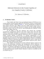
Figure 1 shows a map of Amchitka Island and the location and perspective of
each of the three cross sections representing the simulation domains for the
three tests.
2. PROCESSES MODELED, PARAMETERS, AND CALIBRATION
Modeling Amchitka’s nuclear tests encompasses two major
processes: 1) the flow modeling, taken here to include density-driven flow,

© 2004 by CRC Press LLC
Uncertainty Analysis of Saltwater Intrusion
209


Figure 1: Location of model cross section for each site with the cartoon eye
indicating the perspective of subsequent figures.
saltwater intrusion, and heat-driven flow, and 2) the contaminant transport
modeling, combining radioactive source evaluation and decay, retardation
processes, release functions, and matrix diffusion. The symmetry of island
hydraulics lends itself to considering flow in two dimensions, on a transect

from the hydrologic divide along the island’s centerline, through the nuclear
test location, and on to the sea. The boundary conditions for the flow
problem entail no flow coinciding with the groundwater divide and along the
bottom boundary. The seaward boundary is defined by specified head and
constant concentration equivalent to seawater. The top boundary has two
segments. The portion across the island receives a recharge flux at a
freshwater concentration, and the portion along the ocean is a specified head
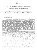
dependent on the bathymetry. Figure 2 shows the Milrow topographic and
bathymetric profile, the domain geometry and boundary conditions, and the
finite element mesh used to discretize the density-driven flow equations. The
mesh is refined in the entire left upper triangle of the simulation domain
since the TZ varies widely with the random parameters selected.
For the other two sites, similar domain geometry and boundary
conditions are utilized. However, the upper boundary is determined based on
the specific site’s topography and bathymetry, which is slightly different

© 2004 by CRC Press LLC
Coastal Aquifer Management
210

Figure 2: Milrow profile that determines (a) the upper boundary of the
simulation domain, and (b) the discretization and boundary conditions.
among the three sites. Island-specific data are used to constrain the parameter
values used to construct the seawater intrusion flow problem. Hydraulic
conductivity, K, data collected from six boreholes are used to yield the best
estimate for a homogeneous conductivity value and the range of uncertainty
associated with this estimate. The geologic environment suggests strong
anisotropy, so that vertical hydraulic conductivity, K
zz
, is assumed to be one-

tenth the horizontal value (except in the chimney above the nuclear cavity,
where collapse is assumed to increase K
zz
relative to that of the horizontal
conductivity, K
xx
). Temperature logs measured in several boreholes and
water balance estimates are used to derive groundwater recharge, R, values.
Measurements of total porosity on almost 200 core samples from four
boreholes provided a mean and distribution for matrix porosity. No
measurements of fracture porosity, a notoriously difficult-to-measure
parameter, are available, so literature values guided that selection. The
transport model also required data on retardation properties, which were
obtained using sorption and diffusion experiments from core material.
© 2004 by CRC Press LLC
Uncertainty Analysis of Saltwater Intrusion
211
The model for each of the nuclear tests was calibrated using site-
specific hydraulic head and water chemistry data. The objective of the
calibration was to select base-case, uniform flow, and saltwater intrusion
parameters that yield a modeling result as close as possible to that observed
in the natural system. Difficulty was encountered in obtaining simultaneous
best-fits to the two targets (head and chemistry). The best parameters to
match head would result in a less perfect match for the chemical profile, and
vice versa. The critical calibration feature for locating the mid-point of the
TZ is the ratio of recharge to hydraulic conductivity (R/K). Macrodispersivity
controlled the width of the TZ modeled around the mid-point. Ultimately,
compromises were made to achieve the optimum fit to both heads and
chemistry, and more weight was given to the hydraulic head measurements
due to reported difficulties encountered in obtaining representative samples

from these very deep boreholes during drilling operations. The configuration
of the seawater interface differs from one site model to another, with a
deeper freshwater lens calculated on the Bering Sea side of the island.
3. PARAMETRIC UNCERTAINTY ANALYSIS
To optimize the modeling process, a parametric uncertainty analysis
was performed to identify which parameters are important to treat as
uncertain in the flow and transport modeling and which to set as constant,
best estimate, values. This analysis was performed for the Milrow site and
the findings are applied to all sites. The processes evaluated through their
flow and transport parameters include recharge, saltwater intrusion,
radionuclide transport, glass dissolution, and matrix diffusion. The end result
of this analysis is a relative comparison of the effect of uncertainty of each
individual parameter on the final transport results in terms of the arrival time
and mass flux of radionuclides crossing the seafloor.
3.1 Uncertainty Analysis of Flow Parameters
The parameters of concern here are the hydraulic conductivity, K,
the recharge, R, and the longitudinal and transverse macrodispersivities, A
L
and A
T
. Since the saltwater intrusion problem encounters a density-driven
flow, the macrodispersivities are considered as flow parameters. In addition,
the porosity is also considered at this stage as the spatial variability of
porosity between the chimney and the surrounding area affects the solution
of the saltwater intrusion problem. In all cases, the flow and the advection-
dispersion equations are solved simultaneously until a steady-state condition
is reached. The solution provides the groundwater velocities and the
concentration distribution that can be used to identify the location and

© 2004 by CRC Press LLC

Coastal Aquifer Management
212

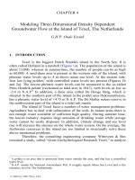
Figure 3: A summary of the two modeling stages and the implementation of
the parametric uncertainty analysis. The numbers in square brackets are for
the scenarios studied in the first modeling stage.
thickness of the TZ. For each of the four parameters, a random distribution of
100 values below and above a “mean” value close to the calibration result is
generated. Figure 3 summarizes the parametric uncertainty analysis for all
© 2004 by CRC Press LLC
Uncertainty Analysis of Saltwater Intrusion
213
parameters (first modeling stage) and the combined uncertainty analysis
(second modeling stage).
For the first modeling stage, a lognormal distribution was used to
generate the recharge values for Scenario 1 and the distribution was
truncated such that the upper and lower limits lead to reasonable TZ
movement around the location indicated by the chemistry data. For Scenario
2, the uncertain conductivity values are generated from a lognormal
distribution and have a mean value of 6.773 × 10
–3
m/day, which is
equivalent to the Milrow calibration value. As for recharge, a lognormal
distribution was selected with upper and lower limits that were consistent
with the data and yielded a reasonable TZ.
From these conductivity limits and those of the recharge, the
recharge-conductivity ratio is changing from 1.35 × 10
–3
to 9.05 × 10
–3

for
Scenario 1 and from 1.26 × 10
–3
to 2.05 × 10
–2
for Scenario 2. It should be
mentioned here that the recharge-conductivity ratio is the factor that controls
the location of the TZ, but the magnitude of the velocity depends on the
recharge and conductivity values. The large macrodispersivity values are
considered to account for the additional mixing resulting from spatial
variability that is not considered in the model and to avoid violation of the
Peclet number if small macrodispersivity values are used. For all cases
considered, the chimney and cavity porosity is set to a fixed value of 0.07,
whereas the rest of the domain is assigned a fracture porosity value that is
obtained from a random distribution having a minimum value of 1.294 × 10
–5

and a maximum value of 3.8 × 10
–3
.
Having generated the individual random distributions for each of the
parameters considered, the variable-fluid-density groundwater flow problem
is solved using the FEFLOW code [Diersch, 1998]. For each one of the four
parameters considered, a set of 100 steady-state velocity and concentration
distributions is obtained that corresponds to the 100 random input values. For
the simulated head and concentration values at the Milrow calibration well,
Uae-2, the mean of the 100 realizations as well as the standard deviation of
the result are computed.
Figures 4 and 5 show the impact of the extreme values of R and K on
the TZ location for Scenarios 1 and 2 that address the uncertainty in R and K,

respectively. The smaller range of R/K is reflected on the TZ locations shown
in Figure 4. Figures 6 and 7 show the sensitivity of the concentration and
head to the uncertainty in the values of recharge and conductivity,
respectively. In each figure, the mean of the Monte Carlo runs, the mean ±
one standard deviation, and the data points are plotted. It can be seen that for
the recharge case, the one standard deviation confidence interval around the
mean captures most of the data points for concentration and for head

© 2004 by CRC Press LLC
Coastal Aquifer Management
214

Figure 4: Transition zone location relative to cavity location for the
extreme values of R in the recharge sensitivity case.
measurements. The conductivity case (Figure 7) covers the high
concentration data (saltwater side) but gives lower concentrations than the
data for the freshwater side of the TZ. The head sensitivity to conductivity
variability shown in Figure 7 indicates that the confidence interval
encompasses all the head data at Uae-2.
The porosity does not affect the solution of the flow problem even
with the chimney having a different porosity. The porosity only influences
the speed at which the system converges to steady state, and as such,
simulated heads and concentrations at Uae-2 do not show any sensitivity to
the fracture porosity value outside the chimney. It should be recognized,
however, that the fracture porosity outside the chimney and cavity area will
have a dramatic effect on travel times and radioactive decay of mass released
from the cavity and migrating toward the seafloor. The range of 60 to 500 m
considered for A
L
has a minor effect on the head and concentration at Uae-2,

especially at the center of the TZ.
Again, the final decision as to whether the uncertainty in a parameter
is important to include in the final modeling stage cannot be determined from
these results. The criterion for selecting the most influential parameters can

© 2004 by CRC Press LLC
Uncertainty Analysis of Saltwater Intrusion
215

Figure 5: Transition zone location relative to the cavity location for the
extreme values of K in the conductivity sensitivity case.
only be determined by analyzing the transport results in terms of travel times
from the cavity to the seafloor and location where breakthrough occurs. The
set of results discussed here indicates that the simulated heads and
concentrations at Uae-2 are most sensitive to conductivity and recharge and
least sensitive to fracture porosity outside the chimney and
macrodispersivity. The parameter importance to the transport results may be
confirmed or changed by analyzing the travel time statistics for particles
originating from the cavity and breaking through the seafloor.
The velocity realizations resulting from the solution of the flow
problem are used to model the radionuclide transport from the cavity toward
the seafloor. The transport parameters are kept fixed at their means while
addressing the effect of the four parameters that change the flow regime.
When the effect of transport parameters, such as matrix diffusion coefficient,
glass dissolution rate, etc., is studied, a single velocity realization with the
flow parameters fixed at the calibration values is used.
© 2004 by CRC Press LLC
Coastal Aquifer Management
216

Figure 6: Sensitivity of modeled concentrations and heads at Uae-2 to the
recharge uncertainty.
3.2 Uncertainty Analysis of Transport Parameters
To analyze the effect of transport parameters’ uncertainty on
transport results, a 100-value random distribution for local dispersivity,
α
L
,
is generated from a lognormal distribution. The analysis is performed using a
single flow realization and the transport simulations are performed for 100
different
α
L
values. A similar analysis is performed to analyze the effect of
the matrix diffusion parameter,
κ
. Based on available data and literature
values, a best estimate for
κ
of 1.37 day
–1/2
was derived. This value leads to
a very strong diffusion into the matrix, which significantly delays the mass
arrival to the seafloor, producing no mass breakthrough at the seafloor within
the selected time frame of about 27,400 years of this first modeling stage. As
there is a large degree of uncertainty in determining this parameter and the
uncertainty derived by the conceptual model assumptions for diffusion (e.g.,
assumption of an infinite matrix), values for
κ
that are smaller than the best

estimate of 1.37 were chosen. A random distribution of 100 values is
generated for
κ
with a minimum of 0.0394, a maximum of 1.372, and a
mean of 0.352.
© 2004 by CRC Press LLC
Uncertainty Analysis of Saltwater Intrusion
217

Figure 7: Sensitivity of modeled concentrations and heads at Uae-2 to the
conductivity uncertainty.
The transport simulations are performed using a standard random
walk particle tracking method [Tompson and Gelhar, 1990; Tompson, 1993;
LaBolle et al., 1996, 2000; Hassan et al., 1997, 1998]. For more details about
the transport simulations that are pertinent to this study, the reader is referred
to Hassan et al. [2001] and Pohlmann et al. [2002].
To show how the particles travel from the cavity to the seafloor
(breakthrough plane), a single realization showing about 100% mass
breakthrough during a time frame of 2,200 years is selected for analysis and
visualization. The particle locations at different times are reported and used
to visualize the plume shape and movement. Figure 8 shows three snapshots
of the particles’ distribution at different times with the percentage mass
reaching the seafloor computed and presented on the figure. No particles
reach the seafloor within the first 100 years after the detonation. At 140
years, the leading edge of the plume starts to arrive at the seafloor. Larger
numbers of particles arrive between 140 and 180 years, with a total of 1.2%
of the initial mass reaching the seafloor by 180 years. For the rest of

© 2004 by CRC Press LLC
Coastal Aquifer Management

218

Figure 8: Snapshots of the particles’ locations showing how the plume moves
along the TZ of the seawater intrusion problem.
simulation time, the accompanying CD for this book contains an animated
movie showing the plume movement as a function of time.
3.3 Results of the Parametric Uncertainty Analysis
The mass flux breakthrough curves resulting from the arrival of
radionuclides to the seafloor are analyzed in terms of the mean arrival time
of the mass that breaks through within the simulation time frame and the
location of this breakthrough along the bathymetric profile. Recall that the
purpose of this analysis is to select the parameters for which the associated
uncertainty has the most significant effect on transport results expressed in
terms of uncertainty of travel time to the seafloor and the location where
© 2004 by CRC Press LLC
Uncertainty Analysis of Saltwater Intrusion
219
breakthrough occurs. By doing so, the parameters for which the uncertainty
only slightly affects the uncertainty in travel time and transverse location of
the breakthrough can be identified, and as such, these parameters are fixed at
their best estimate and only those with significant effects are varied.
The results of the sensitivity analysis performed for the six
parameters, K, R,
θ
, A
L
(in saltwater intrusion), a
L
(in radionuclide transport
modeling), and

κ
are summarized in Table 1, in which the matrix diffusion
parameter,
κ
, is assigned the value of 0.0434 day
–1/2
that is one order of
magnitude lower than the base-case value. This is because the base-case
value leads to significant matrix diffusion that conceals the different
uncertainty effects. Reducing the effect of matrix diffusion allows for a
comparison between different uncertainties and their impact on the transport
results. For each case, the table presents the range of values of the input
parameter (minimum, maximum, and mean), the standard deviation, and the
coefficient of variation. On the output side, the results are presented in terms
of the statistics of travel time and transverse location where breakthrough
occurs. For each single realization of the radionuclide transport, the mean
arrival time and mean transverse location of the mass that has crossed the
seafloor within 27,400 years are recorded. The resulting ensemble of these
values is used to compute the mean, standard deviation, and coefficient of
variation of the travel time and location, which are presented in Table 1.
To facilitate the comparison between different cases, one would
compare the values of the coefficient of variation on both input and output
sides. Among the six cases in Table 1, the two cases encountering variability
in the macro/local dispersivity value lead to very small uncertainty in the
travel time and the transverse location in comparison to other parameters.
Although the coefficient of variation of a
L
in radionuclide transport
simulations is higher than that of conductivity and recharge, the resulting
coefficients of variation for travel time and transverse location are much

smaller. Therefore, it can be argued that the uncertainty in these two
parameters may be neglected, as their variabilities slightly influence
transport results when compared to other parameters. This leaves the four
parameters, K, R,
θ
, and
κ
. The fracture porosity variability with the highest
coefficient of variation among these four parameters leads to the highest
variability in mean arrival time. The conductivity, on the other hand, leads to
the highest variability in transverse location. The first three parameters of
this reduced list influence the solution of the flow problem and thus require
multiple realizations of the flow field. The matrix diffusion parameter is a
transport parameter that does not require multiple flow realizations.

© 2004 by CRC Press LLC
Coastal Aquifer Management
220
Table 1: Results of the uncertainty analysis comparing the effects of different
parameters on plume travel time and transverse location of the breakthrough.
The final choice for the uncertain parameters for the second
modeling stage is the three flow parameters. This choice is motivated by the
fact that the available data only pertain to the solution of the flow problem
and can be used to guide the generation of the random distributions in the
second stage. Head and chloride concentration data can be used as criteria for
determining whether the combined random distributions lead to realistic flow
solutions or not. Given that using the same random distribution for
κ
as in
the first stage or skewing it toward higher or lower values cannot be judged

or tested against data, the transport results are obtained using a conservative
estimate for the
κ
, which is kept constant in all subsequent analysis.
3.4 Flow and Transport Results of the Second Modeling Stage
For the primary flow and transport modeling for the sites, using the
significant uncertain parameters identified in the parametric uncertainty
analysis (K, R, and
θ
), the same model meshes employed in the individual
parametric uncertainty analysis are used. Three new random distributions are
generated for the conductivity, recharge, and fracture porosity for each site
with the total number of realizations between 240 and 300. Flow and
Parameters

K
(m/d)
R
(cm/y)
A
L

(m)
θ

(-)
α
L
(m)
κ

(d
-1/2
)
Min
0.89µ10
-3
0.328

62

1.3µ10
-3
0.56 0.039
Mean
6.77µ10
-3
1.125 300
5.2µ10
-3

5.0 0.352
Max
2.45µ10
-2
2.205 500
3.8µ10
-3

19.5 1.37
σ

4.34µ10
-3
0.475

82 6.4µ10
-4
3.45 0.243
Input
Statistics
cv 0.641 0.422 0.27 1.23 0.69 0.691
Mean 22.19 22.00 20.65 19.101 23.0 25.77
σ
1.98

3.484

0.742 4.965

0.31 1.15
Travel
Time
(10
3

years)
cv 0.089 0.158 0.036 0.260 0.01 0.045
Mean 3.629 3.404 3.394 3.382 3.37 3.274
σ
0.660 0.375 0.009 0.042 0.02 0.031
BT

Location
(km)
cv 0.182 0.110 0.003 0.012 0.01 0.009
© 2004 by CRC Press LLC
Uncertainty Analysis of Saltwater Intrusion
221
transport simulations are performed in a manner similar to the first stage. The
output presented here is a point mass flux distribution as a function of space
and time, q(x, t), where q is the mass crossing a unit cross-sectional area per
unit time, x is the horizontal distance along the seafloor relative to the island
center (or groundwater divide), and t is the time since the migration started.
This two-dimensional distribution of q is obtained for each individual
realization and the ensemble mean, <q>, is obtained by averaging over all
realizations for each site.
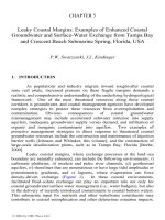
Figure 9 shows the transport results for the three sites with Milrow in
the top plot, Cannikin in the middle plot, and Long Shot in the lower plot. In
each plot, the cavity location (source of radionuclides) and the TZ locations
associated with the extreme values of R/K among all realizations are shown.
The plots also show the space-time distribution of the ensemble mean of the
point mass flux, < q(x, t) >, for carbon-14 (half life = 5,730 years) with the
right axis indicating time. This plot is superimposed on the TZ plots to show
the location where breakthrough occurs relative to the cavity location and the
limits of the TZ location produced by the uncertain input parameters.
The figure shows that the incorporation of uncertainty in the TZ
location (through uncertainty in recharge and hydraulic conductivity),
combined with the different location of the test cavity between the three
sites, leads to a large variation in transport results from one test to the other.
The transport results calculated for a realization with the cavity intersecting
the TZ is dramatically different than for a realization with the TZ below the
cavity. For both Milrow and Cannikin, the early-time portion of the mass

flux breakthrough is dominated by the realizations representing the transition
zone at or below the cavities. Based on the results shown in Figure 10, the
Long Shot cavity is always located at the freshwater side and very far from
the center of the transition zone. This leads to the direct movement of
radionuclides from the cavity toward the seafloor. The Milrow cavity and
that of Cannikin, on the other hand, are located at the saltwater side of the TZ
in many realizations. This means that in these realizations, the cavity comes
in contact with the very slow flow pattern occurring at the lower edge of the
TZ. This explains why a number of realizations at Milrow and Cannikin do
not produce any mass breakthrough within 2,200 years. For Cannikin, the
cavity is deeper than that for Milrow. This results in a longer flow path to
the seafloor, thereby causing breakthrough to occur at a later time and with
smaller mass flux values than Milrow due to the increased radioactive decay.
The location of the breakthrough is mainly dominated by the cavity location;
thus it can be seen that the breakthrough at Long Shot is closest to the
shoreline followed by that of Milrow and then Cannikin.

© 2004 by CRC Press LLC
Coastal Aquifer Management
222

Figure 9: Expected value of point mass flux, < q(x, t) >, at the three sites as a
function of breakthrough time (right vertical axis) and location (horizontal
axis). The TZ location (left vertical axis and horizontal axis) for maximum
and minimum values of R/K is shown to relate to the cavity location and the
breakthrough location.
© 2004 by CRC Press LLC
Uncertainty Analysis of Saltwater Intrusion
223
Table 2: Values of parameters used in FEFLOW for simulations

incorporating geothermal heat.
4. SENSITIVITY STUDIES
Numerical modeling of the coastal aquifer systems at Amchitka
Island directly incorporates uncertainties in critical parameters where data
allow. However, some uncertainties cannot be addressed through that
process, either due to lack of data, or because the uncertainty is in the
underlying conceptual model or numerical approach. These uncertainties are
addressed through separate sensitivity studies and are discussed in the
following sections.
4.1 Geothermal Heat
The base-case flow models are run under isothermal conditions,
assuming that compared to geothermal effects, the freshwater–seawater
dynamics dominate the island flow system. The impacts of including
geothermal heat are addressed through a nonisothermal analysis of the
Milrow flow system, where hydraulic head, concentration, and temperature
data sets are most complete and reliable.

The geothermal model simulates pre-nuclear test conditions;
therefore, the chimney is not included and K and
θ
are treated as
homogeneous properties throughout the domain. With the exceptions noted
below, values of the groundwater flow parameters are the same as the values
used in the calibrated flow model of Milrow. The values of the parameters
required for the geothermal component are listed in Table 2. Fluid density
and viscosity are dependent on both concentration and temperature, based on
a nonlinear relationship of density to temperature incorporated in the
FEFLOW code. Rock thermal properties are based on core samples from the
island [Green, 1965]. The thermal properties of water are FEFLOW default
values. The temperature of 125°C at the bottom boundary is extrapolated

Parameter Value
Rock Volumetric Heat Capacity,
ρ
s
c
s
1.9 µ 10
6
J/m
3
C
Water Volumetric Heat Capacity,
ρ
0
c
0
4.2 J/m
3
C
Rock Thermal Conductivity,
λ
s
2.59 J/m
3
C
Water Thermal Conductivity,
λ
0
0.56 J/m

3
C
Thermal Longitudinal Dispersivity,
β
L
100 m
Thermal Transverse Dispersivity,
β
T
10 m
Water Density and Viscosity,
ρ
0
and
µ
0
6th order function of
temperature
© 2004 by CRC Press LLC
Coastal Aquifer Management
224

Figure 10: Effect of the inclusion of geothermal heat (A) and island half
width, IHW (B) on the two-dimensional TZ at Milrow.
from temperature profiles measured in several Amchitka boreholes [Sass and
Moses, 1969], and indicates a geothermal gradient of 3.2°C per 100 m depth.
The temperature at the upper boundary is 4°C, which is consistent with both
the mean average air temperature noted for Amchitka [Armstrong, 1977] and
the value for ground surface extrapolated from the subsurface temperature
profiles.

The results indicate that thermally driven buoyant flow caused by the
geothermal gradient increases the vertical upward flux below the island and
shifts the transition zone almost 200 m higher relative to the isothermal case
(Figure 10A). At the TZ, this increased vertical flux is then directed seaward,
resulting in higher velocities along the TZ as compared to the isothermal
case. Despite these differences, the overall patterns of flow are similar to the
isothermal case. The upward and left (toward the divide) components of
© 2004 by CRC Press LLC
Uncertainty Analysis of Saltwater Intrusion
225
velocities simulated below the TZ are both larger due to the buoyancy-driven
flow simulated in the geothermal model. Higher flow rates mean that
velocities near the working point, which is located below the TZ at Milrow,
are higher when including the effects of geothermal heat. The vertical and
horizontal velocities at the Milrow working point are about twofold higher in
the geothermal model. Velocities higher than the isothermal model are
generally maintained along the predicted flowpaths from the working point
toward the sea, suggesting that inclusion of geothermal heat in the model
simulations has the effect of reducing contaminant travel times for the
Milrow and Cannikin sites where the working points are below the TZ in
many of the realizations considered.
4.2 Island Half-Width
The conceptual model for groundwater flow at Amchitka assumes
that a groundwater divide runs along the long axis of the island, separating
flow to the Bering Sea on one side and flow to the Pacific Ocean on the other
(see Figure 1). The position of the divide is also assumed to coincide with
that of the surface water divide. This assumption can be called into question
due to the observation of asymmetry in the freshwater lens beneath the island
[Fenske, 1972a, b]. This asymmetry is supported by the data analysis and

modeling performed here, which suggests that the freshwater lens is deeper
at Long Shot and Cannikin than at Milrow.
Not only is there uncertainty as to whether the groundwater and
surface water divides coincide, there is additional uncertainty in the location
of the surface water divide itself, as the topography of the island in the area
of the nuclear tests is very subdued. The surface water divide was estimated
using a detailed series of topographic maps at a scale 1:6,000 and with a 10-
foot contour interval. Despite this resolution, the distance between 10-foot
elevation contours can reach over 100 m in places.
To understand the impact of this uncertainty on the groundwater
modeling, several sensitivity cases were evaluated. In these, the island half-
width was assumed to be 200 and 400 m wider than the estimate for Milrow,
and also assumed to be 200 and 400 m narrower than used in the base-case
model. For reference, the base-case half-width used at Milrow is 2,062 m, so
that plus and minus 10 and 20% differences are considered here. One
realization was used for these calculations, one in which the cavity is located
in the freshwater lens. It shows a 100% mass breakthrough and has the
parameter values K = 2.34 × 10
–2
m/d, R = 1.82 cm/yr, and
θ
= 1.62 × 10
–4
.
Varying the island half-width both affects the depth to the TZ
(through varying the land surface available for recharge) and the position of
the cavity in the flow system (by virtue of changing the distance from the test
to the no-flow boundary). The TZ depicted from the vertical chloride
© 2004 by CRC Press LLC
Coastal Aquifer Management

226
concentrations in the Uae-2 well at Milrow is plotted in Figure 10B for the
base-case island width and the four additional sensitivity cases. Reducing the
island half-width decreases the depth of the TZ, and cuts the distance
between the cavity and the transition in half for the 400-m-shorter half-
width. Conversely, the TZ is deepened by an increasing half-width,
increasing the distance from the cavity to the TZ by a factor of two for the
400-m-wide island. The flowpath distance to the seafloor from the cavity is
also affected, lengthening for a wider island and shrinking for a smaller one.
The impact of these various configurations on transport is also
investigated. It is found that the 400-m-longer half-width leads to an earlier
breakthrough of mass at a peak flux about two times larger than the base
case. On the other hand, the 400-m-shorter half-width results in a delay in
breakthrough at a peak mass about five times lower than the base case.
4.3 Dimensionality of Rubble Chimney
The models used in the uncertainty analysis utilize a two-
dimensional perspective to analyze the flow and transport problem, a
simplification that is consistent with the island hydraulic environment. This
simplifying assumption is considered reasonable for the conceptual model
and is significantly more computationally efficient than a fully three-
dimensional formulation. However, the two-dimensional formulation
accounts for the geometry of the rubble chimney only in the plane of the
model, i.e., parallel to the natural flow direction, and therefore the chimney is
simulated as extending infinitely in the direction perpendicular to the plane
of the model. In reality, the chimney is a vertical columnar feature in a three-
dimensional flow field that is only as wide perpendicular as it is parallel to
natural flow.

The three-dimensional model builds on the Cannikin two-
dimensional model by simply extending the domain in the direction of the

island shoreline (perpendicular to the axes of the two-dimensional model).
Thus, the finite-element mesh geometry of each vertical slice in the three-
dimensional model is identical to the mesh geometry of the two-dimensional
Cannikin model, with each element now having a constant width in the y
direction (Figure 11).
The impacts of flow in a three-dimensional rubble chimney are
simulated in a model 1,500 m wide, i.e., perpendicular to the natural flow
direction (Figure 11). The chimney is simulated as a vertical column
extending to ground surface that is rectangular in cross section and has a
width of about two R
c
, where R
c
is the cavity radius (estimated to be 157 m).
The hydraulic properties of the rock outside the chimney are considered to be


© 2004 by CRC Press LLC
Uncertainty Analysis of Saltwater Intrusion
227

Figure 11: Mesh configuration used for simulations of the rubble chimney.
Table 3: Values of parameters used in the three-dimensional rubble chimney
simulations.
not significantly affected by the nuclear explosion and are assigned the
background values of K and porosity. Model parameters that differ from the
base-case Cannikin model for the three realizations are shown in Table 3.
The sensitivity studies are applied to three realizations selected out
of the 260 runs for the Cannikin two-dimensional model. The parameter
combinations of these realizations encompass a variety of positions of the TZ

Parameter Case #1 Case #2 Case #3
K
xx
, K
yy
(m/d)
1.86×10
-2
6.48×10
-2
1.78×10
-2

K
zz
(m/d)
1.86×10
-3
6.48×10
-3
1.78×10
-3

K
xx
, K
yy
, K
zz

of cavity and
chimney (m/d)
1.86×10
-2
6.48×10
-2
1.78×10
-2

Rech (cm/yr) 6.13 3.33 1.89
θ
f

2.81×10
-4
2.71×10
-4
2.67×10
-4

© 2004 by CRC Press LLC
Coastal Aquifer Management
228



Figure 12: Comparison of vertical profiles of chloride concentration (mg/L)
for two-dimensional and three-dimensional representations of the island
hydraulics for the three selected realizations.
relative to the test cavity, while having virtually identical porosity (about

2.67 × 10
–4
). Because the velocity field is very sensitive to porosity, this
parameter was held constant to highlight the impact of the sensitivity cases.
Though these realizations were selected from the realizations generated for
Cannikin, the various positions of the TZ relative to the cavity allow them to
represent flow fields possible for all three sites. The realization with the TZ
well below the cavity is representative of Long Shot. The realizations with
© 2004 by CRC Press LLC
Uncertainty Analysis of Saltwater Intrusion
229
the cavity within and below the TZ are likely to be more representative of
Milrow and Cannikin.
Simulation of the rubble chimney in three dimensions results in the
simulation of a shallower TZ as compared to the two-dimensional case with
the same parameter values (Figure 12). The magnitude of the difference is
greatest for the highest R/K ratio, which places the TZ higher by about 500
m. Despite this, the test cavity remains well within the freshwater lens for
this realization and thus flow velocities from the cavity are not impacted
significantly. The inclusion of the three-dimensional rubble chimney for the
lower R/K ratio places the TZ about 100 m higher, placing the cavity further
into the low velocity saltwater zone.
The greater flux through the chimney and the radial flow in three
dimensions introduce into the model a mechanism for lateral spreading of
contaminants originating in the cavity that is not present in the two-
dimensional model. The net effect is lower contaminant concentrations as the
plume is diluted with a larger volume of groundwater. The result is that the
two-dimensional model underestimates the effect of the chimney on slowing
groundwater velocities and neglects dispersion in the third dimension. This
result is true for all three R/K ratios and indicates that the use of the two-

dimensional approximation for transport from the cavities is a conservative
approach.
5. CONCLUDING REMARKS
The uncertainty analysis for Amchitka Island not only provides
information for a theoretical analysis of the importance and interplay among
flow and transport parameters in coastal aquifers, it provides valuable
information for managing this site of groundwater contamination.
Uncertainty always exists when considering subsurface problems;
quantifying the impact of that uncertainty on contaminant transport
predictions can allow site managers to decide whether the uncertainty can be
tolerated or must be reduced through additional data collection. Including the
results of uncertainty (through a standard deviation on the breakthrough
curves) always increases predicted transport. If a decision is made to reduce
the uncertainty, the type of analysis shown here provides a quantitative
framework for designing a field program with the highest chance of reducing
model prediction uncertainty.

© 2004 by CRC Press LLC
Coastal Aquifer Management
230
REFFERENCES
Armstrong, R.H., “Weather and climate,” In: The Environment of Amchitka
Island, Alaska, eds. M.L. Merritt and R.G. Fuller, 53–58, Energy
Research and Development Administration, Technical Information
Center, 1977.
Diersch, J.J., “Interactive, graphics-based finite-element simulation system
FEFLOW for modeling groundwater flow contaminant mass and
heat transport processes, FEFLOW Reference Manual,” WASY Ltd.,
Berlin, 294 p., 1998.
Fenske, P.R., “Event-related hydrology and radionuclide transport at the

Cannikin Site, Amchitka Island, Alaska,” Desert Research Institute,
Water Resources Center, Report 45001,NVO-1253-1, 41 p., 1972a.
Fenske, P.R., “Hydrology and radionuclide transport, Amchitka Island,
Alaska,” Desert Research Institute, Technical Report Series H-W,
Hydrology and Water Resources Publication No. 12, 29 p., 1972b.
Green, G.W., “Some hydrological implications of temperature measurements
in exploratory drillholes, Project Long Shot, Amchitka Island,
Alaska,” U.S. Geological Survey Technical Letter Goethermal—1, 8
p., 1965.
Hassan, A.E., Cushman, J.H. and Delleur, J. W., “Monte Carlo studies of
flow and transport in fractal conductivity fields: Comparison with
stochastic perturbation theory,” Water Resources Research, 33(11),
2519–2534, 1997.
Hassan, A.E., Cushman, J.H. and Delleur, J. W., “A Monte Carlo assessment
of Eulerian flow and transport perturbation models,” Water
Resources Research, 34(5), 1143–1163, 1998.
Hassan, A.E., Andricevic, R. and Cvetkovic, V., “Computational issues in
the determination of solute discharge moments and implications for
comparison to analytical solutions, Advances in Water Resources,
24, 607–619, 2001.
LaBolle, E., Quastel, J., Fogg, G. and Gravner, J., “Diffusion processes in
composite porous media and their integration by random walks:
Generalized stochastic differential equations with discontinuous
coefficients,” Water Resources Research, 36(3), 651–662, 2000.
LaBolle, E., Fogg, G. and Tompson, A.F.B., “Random-walk simulation of
solute transport in heterogeneous porous media: Local mass-
conservation problem and implementation methods,” Water
Resources Research, 32(3), 583–593, 1996.

© 2004 by CRC Press LLC
Uncertainty Analysis of Saltwater Intrusion
231
Pohlmann, K.F., Hassan, A.E. and Chapman, J.B., “Modeling density-driven
flow and radionuclide transport at an underground nuclear test:
Uncertainty analysis and effect of parameter correlation,” Water
Resources Research, 38(5), 10.1029/2001WR001047, 2002.
Sass, J.H. and Moses, T.H., Jr., “Subsurface temperatures from Amchitka
Island, Alaska,” U.S. Geological Survey, Technical Letter, USGS
474-20 (Amchitka-16), 5 p., 1969.
Tompson, A.F.B. and Gelhar, L.W., “Numerical simulation of solute
transport in three-dimensional, randomly heterogeneous porous
media,” Water Resources Research, 26(10), 2451–2562, 1990.
Tompson, A.F.B., “Numerical simulation of chemical migration in
physically and chemically heterogeneous porous media,” Water
Resources Research, 29(11), 3709–3726,1993.
© 2004 by CRC Press LLC