Handbook of Ecological Indicators for Assessment of Ecosystem Health - Chapter 5 doc
Bạn đang xem bản rút gọn của tài liệu. Xem và tải ngay bản đầy đủ của tài liệu tại đây (1.18 MB, 35 trang )
CHAPTER 5
Application of Ecological and
Thermodynamic Indicators for the
Assessment of Lake Ecosystem Health
Fu-Liu Xu
A tentative theoretical frame, a set of ecological and thermodynamic
indicators, and three methods have been proposed for the assessment of lake
ecosystem health in this chapter. The tentative theoretical frame includes five
necessary steps: (1) the identification of anthropogenic stresses; (2) the analysis
of ecosystem responses to the stresses; (3) the development of indicators; (4)
the determination of assessment methods; and (5) the qualitative and
quantitative assessment of lake ecosystem health. A set of ecological and
thermodynamic indicators covering lake structural, functional, and system-
level aspects were developed, according to the structural, functional, and
system-level responses of 59 actual and 20 experimental lake ecosystems to the
5 kinds of anthropogenic stresses: eutrophication, acidification, heavy metals,
pesticides, and oil pollution. Three methods are proposed for lake ecosystem
health assessment: (1) the direct measurement method (DMM); (2) the
ecological modeling method (EMM); and (3) the ecosystem health index
method (EHIM). These indicators and methods were successfully applied to
the assessment and comparison of ecosystem health for a Chinese lake and
30 Italian lakes.
Copyright © 2005 by Taylor & Francis
5.1 INTRODUCTION
5.1.1 Ecosystem Type and Problem
Lakes are extremely important storage areas for the earth’s surface
freshwater, with important ecosystem service functions that can keep the
development of society and economy sustainable.
1,2
However, eutrophication
and acidification, as well as heavy metal, oil and pesticide pollution caused by
human activities have deteriorated continuously the healthy status of lake
ecosystems. The water in over half of the lakes around the world has been
seriously polluted. If this trend continues, it will not only affect human health
and socio-economic development, but may also cause the breakup of lake
ecosystems altogether.
3,4
Studies on lake ecosystem health therefore have
important and practical significance for the restoration of ecosystem health
and the maintenance of their ecological service functions.
Since the mid-1980s, studies on lake ecosystem health have begun to attract
the attention of environmentalists and ecologists, with increa singly frequent
use in academic and government publications as well as the popular media.
5
More and more environmental managers consider the protection of ecosystem
health as a new goal of environmental management.
6–11
In the past few years,
many national and international environmental programs have been estab-
lished. One of these leading programs is ‘‘Assessing the State of Ecosystem
Health in the Great Lakes,’’ supported by the Canadian and U.S. gov ern-
ments.
12
In the U.S., important ongoing programs related to lake ecosystem
health include mainly ‘‘Assessing Health State of Main Ecosystems,’’
11
and
‘‘Stresses on Ecosystem Health — Chemical Pollution.’’
13
In Canada, an
ongoing key program related to lake ecosystem health is the ‘‘Aquatic
Ecosystem Health Assessment Project.’’
14
In China, special attention has
also been paid to lake ecosystem health. Two projects have been carried out,
namely ‘‘The Effects of Typical Chemical Pollution on Aquatic Ecosystem
Health,’’
15
and ‘‘The Indicators and Methods for Lake Ecosystem Assess-
ment,’’
16,17
Ongoing programs supported by the Natural Science Foundation
of China (NSFC) include ‘‘The Limiting Factors and Dynamic Mechanism
for Lake Ecosystem Health’’; ‘‘Regional Differentia and its Mechanisms for
the Ecosystem Health of Large Shallow Lakes’’; and ‘‘Assessment and
Management of Watershed Ecosystem Health.’’
18
So far, a number of indicators have been proposed for lake ecosystem
health assessment; for example, gross ecosystem product (GEP),
19
ecosystem
stress indicators,
20
the index of biotic integrity (IBI),
21
thermodynamic
indicators including exergy and structural exergy,
22,23
and a set of compre-
hensive ecological indicators covering structural, functional and system-level
aspects.
15,16
Some methods or procedures have also been proposed for
assessing lake ecosystem health; for example, a tentative procedure by
Jørgensen,
23
and the direct measurement method (DMM) and ecological
model method (EMM) by Xu et al.
16,17
However, owing to the lack of criteria,
it causes two major problems using present methods to assess lake ecosystem
Copyright © 2005 by Taylor & Francis
health. First, we can only assess the relative healthy status — it is extremely
difficult to assess the actual health status. Second, it is impossible to make the
comparisons of ecosystem health status for different lakes. In order to solve
these problems, a new method, the ecosystem health index method (EHIM), is
developed in this chapter.
5.1.2 The Chapter’s Focus
This chapter focuses on indicators and methods for assessing lake
ecosystem health, followed by an examination of two case studies. Also, a
tentative theoretical frame or procedure for assessing lake ecosystem health is
proposed. The discussions on indicators, methods, and the results of case
studies are then presented.
5.2 METHODOLOGIES
5.2.1 A Theoretical Frame
A tentative theoretical frame or procedure for assessing lake ecosystem
health is shown in Figure 5.1. It shows that there are five necessary steps in
which the development of indicators and the determination of assessment
methods are two key steps. However, in order to develop sensitive indicators,
the anthropogenic stresses have to be identified, and the responses of lake
ecosystems to the stresses have to be analyzed, since the stresses caused by
human activities are mainly responsible to the degradation of lake ecosystem
health.
Figure 5.1 A tentative procedure for assessing lake ecosystem health.
Copyright © 2005 by Taylor & Francis
5.2.2 Development of Indicators
5.2.2.1 The Procedure for Developing Indicators
The flow chart for developing indicators is shown in Figure 5.2. It can be
seen that the anthropogenic stresses identified to the lake ecosystems include
eutrophication and acidification, as well as heavy metal, pesti cide, and oil
pollution. The lake ecosystems studied should include actual and experimental
anthropogenic stresses. The response of lake ecosystems to the stresses should
be composed of structural, functional, and system-level aspects.
5.2.2.2. Lake Data for Developing Indicators
The actual lake ecosystems (including 29 Chinese lakes (Figure 5.3) and 30
Italian lakes (Table 5.1)) were applied for eutrophication, while the 20
experimental lake ecosystems were chosen because of their eutrophicated
conditions, as well as heavy metals, pesticides and oil pollution (Table 5.2).
It can be seen from Figure 5.3 that 29 Chinese lakes distribute in different
regions in China. Their surface areas range from the 3.7 km
2
Lake Xuanwu-Hu
to 4200 km
2
Lake Qinghai-Hu. Their trophic status are from oligotrophic (e.g.,
Lake Qinghai-Hu) to extremely hypertrophic (e.g., Lake Liuhua-Hu, Lake
Dongshan-Hu and Lake Dong-Hu).
Thirty Italian lakes are located on Sicily. About 70% of the lakes are used
for irrigation; while 30% lakes are used for drinking. Their mean depths are
between 1.5 and 19 m. Their surface area ranges from 1 to 577 km
2
with
average volume varying from 0.1 to 154 billion m
3
.
Experimental ecosystems, including microcosms, mesocosms, and experi-
mental ponds, have been increasingly used in the research on the toxicity and
impacts of chemicals on aquatic ecosystems during the last two decades.
Experimental ecosystem perturbations allow us to separate the effects of
Figure 5.2 A flow chart for developing indicators for lake ecosystem health assessment.
Copyright © 2005 by Taylor & Francis
various pollutants, to assess early effects of perturbations in systems with
known background properties, and to assess quantitatively the result of known
perturbations to whole ecosystems.
25,26
The experimental ecosystems for
developing indicators include 2 microcosms, 14 mesocosms, and 4 experimental
ponds; and the experimental perturbations include acidification, oil, copper,
and organic chemical contamination (Table 5.2).
5.2.2.3 Responses of Lake Ecosystems to Chemical Stresses
Xu et al. exami ned the structural, functional, and ecosystem-level
symptoms resulting from chemical stress, acidification, and copper, oil, and
pesticide contamination in lake ecosystems, based on the above-mentioned
data on experimental ecosystems.
15
They concluded that the structural
responses of freshwater ecosystems to chemical stresses were noticeable in
terms of an increase in phytoplankton cell size and phytoplankton and
microzooplankton biomass, and a decrease in zooplankton body size,
zooplankton and macrozooplankton biomass and species diversity, and in
the zooplankton/phyt oplankton and macrozooplankton/microzooplankton
ratios. The functional responses included decreases in alga C assimilation,
Figure 5.3 Geographic locations of 29 Chinese lakes used for developing indicators. MX1:
Lake Wulungu-Hu; MX2: Lake Beshiteng-Hu; MX3: Lake Wuliangshu-Hai; MX4:
Lake Huashu-Hai; MX5: Lake Dai-Hai; MX6: Hulun-Hu; DB1: Lake Wudalianchi;
DB2: Lake Jingbe-Hu; DB3: Lake Xiaoxingkai-Hu; DB4: Lake Daxingkai-Hu; QZ1:
Lake Zhaling-Hu; QZ2: Lake Eling-Hu; QZ3: Lake Qinghai-Hu; YG1: Lake Erhai;
YG2:
Lake Fuxian-Hu; PY1: Lake Nanshi-Hu; PY2: Lake Hongzhe-Hu; PY3: Lake
Chao-Hu; PY4: Lake Baoan-Hu; PY5: Lake Hong-Hu; PY6: Lake Tai-Hu; CS1:
Lake Dian-Chi; CS2: Lake Liuhua-Hu; CS3: Lake Dongshan-Hu; CS4: Lake Lu-Hu;
CS3: Lake Dong-Hu; CS6: Lake Xi-Hu; CS7: Lake Xuanwu-Hu; CS8: Lake
Nan-Hu.
Copyright © 2005 by Taylor & Francis
resource use efficiency, the P/B (Gross production/Standing crop biomass) and
B/E (Biomass supported/unit energy flow) ratios, an increase in community
production, and a departure from 1 for the P/R (Gross production/communi ty
respiration) ratio (see Equation 5.3 to Equation 5.5 below for definitions).
System-level responses included decreases in exergy, structural exergy, and
ecological buffering capacities.
15,16
Xu investigated the structural responses of the Lake Chao to eutrophi-
cation.
27
He found that with an increasing eutrophication gradient, algal cell
number and biomass were increased, while algal biodiversity, zooplankton
biomass and the ratio of zooplankton biomass to algal biomass were decreased.
Xu
28
and Lu
29
studied the structural, functional, and system-level responses
of 29 Chinese lakes and 30 Italian lakes to eutrophication, respectively. The
results are summ arized in Table 5.3 and are very similar to the results from
the experimental lake ecosystems stressed by acidification, and heavy metal,
oil and pesticide pollution, with the exemption of zooplankton biomass
and exergy for lakes with the trophic states from oligo-eutrophication to
eutrophication.
Table 5.1 Basic limnological characteristics for 30 Italian lakes
Lake name
Cond.
(mS/cm)
TP
(mg/l)
N-NH
4
(mg/l)
N-NO
3
(mg/l)
SiO
2
(mg/l)
Ancipa 0.18 30.66 12 77 2.0
Arancio 0.72 166.65 667 676 4.8
Biviere di Cesro 0.08 46.02 31 76 0.6
Biviere di Gela 2.72 45.15 22 78 2.3
Castello 0.96 109.88 775 263 2.9
Cimia 2.15 49.57 199 803 4.0
Comunelli 2.51 45.33 331 129 3.4
Dirillo 0.53 60.54 60 514 4.1
Disueri 1.21 1093.43 684 2226 3.6
Fanaco 0.53 54.34 199 1143 3.3
Gammauta 0.49 183.07 154 446 2.7
Garcia 0.77 51.36 22 1165 3.6
Gorgo 4.51 80.87 33 65 6.1
Guadalani 0.42 38.89 111 459 0.3
Nicoletti 1.42 35.18 46 66 1.5
Ogliastro 2.72 40.87 173 1710 2.9
Olivo 0.91 38.00 71 69 1.6
Pergusa 33.65 87.97 788 157 1.6
Piana degli Albanesi 0.37 46.77 349 412 0.4
Piana del Leone 0.41 46.85 160 546 2.4
Poma 0.74 51.11 73 994 1.4
Pozzillo 1.13 49.38 91 355 1.6
Prizzi 0.46 52.99 86 503 2.5
Rubino 1.05 28.94 18 711 1.0
San Giovanni 1.49 80.56 658 283 2.7
Santa Rosalia 0.42 55.81 125 279 3.4
Scanzano 0.50 61.65 300 1283 2.3
Soprano 1.85 2962.96 7671 57 12.7
Trinita 1.86 83.24 26 417 3.8
Vasca Ogliastro 0.32 106.69 28 177 3.4
Villarsosa 2.27 64.06 524 276 1.0
Copyright © 2005 by Taylor & Francis
Table 5.2 The studies on the responses of lake ecosystems to experimental perturbations
Stressors Study type* Location Duration (days) Reference**
Acidification Meso. West Virginia 75 [54]
Acidification Meso. California 35 [55]
Acidification Meso. Ohio 10 [56]
Acidification Meso Ohio 35 [57]
Copper Meso. Ohio 4 [58]
Copper Meso. Ohio 14 [59]
Oil EP Tennessee 420 [60]
Dursban EP California 90 [61]
2,4D-DMA EP Missouri 56 [62]
TCP Meso. Neuherberg 24 [63]
PCP Meso. Neuherberg 24 [63]
Trichloroethylene Meso. Southern Germany 44 [64]
TCB Meso. Southern Germany 22 [65]
Benzene Meso. Western Germany 26 [66]
Atrazine Micro. New Mexico 365 [67]
HCBP Micro New Mexico 365 [67]
Permethrin Meso. Tsukuba, Japan 30 [68]
Hexazinone Meso. Ontario 77 [69], [70]
Bifenthrin EP New Jersey 8 [71]
Carbaryl Meso. Ohio 4 [58]
*Micro. ¼Microcosms; Meso. ¼Mesocosms; EP ¼ Experimental Ponds.
**For acidification see [72]–[75]; For oil pollution see [76]–[79]; for copper pollution see
[80]–[84]; for pesticide pollution see [85]–[90].
Modified from Xu, et al. Ecol. Model. 116, 80, 1999. With permission.
Table 5.3 The structural, functional, and system-level responses of actual lake ecosystems to
eutrophication*
Responses indicators
Dynamics in lake trophic states
Oligo-
eutrophication —
Eutrophication
Eutrophication —
Hyper-
eutrophication
Structural
responses
Phytoplankton cell number
a,b
Increase Increase
Phytoplankton biomass (BA)
a,b
Increase Increase
Phytoplankton cell size
a,b
Increase Increase
Phytoplankton diversity
a
Decrease Decrease
Zooplankton biomass (BZ)
a,b
Increase Decrease
Zooplankton body size
a,b
Decrease Decrease
Zooplankton diversity
a
Decrease Decrease
BZ/BA ratio
a,b
Decrease Decrease
BZmacro./BZmicro. Ratio
a,b
Decrease Decrease
Functional
responses
Phytoplankton primary production
a
Increase Increase
P/B ratio
a
% 1 <0.5
P/R ratio
a
% 1 <1.0
System-level
responses
Exergy
a,b
Increase Decrease
Structural exergy
a,b
Decrease Decrease
*:please see References 28 and 29 for details.
a
for 29 Chinese lakes;
b
for 30 Italian lakes.
Copyright © 2005 by Taylor & Francis
5.2.2.4 Indicators for Lake Ecosystem Health Assessment
Ecological indicators for lake ecosystem health assessment resulting from
chemical stress are important for both the early warning signs of ecosystem
malfunction and confirmation of the presence of a significant ecosystem
pathology.
9,20
Ecological indicators as valid and reliable tools should include
structural, functi onal, and system-level aspects. According to the above-
mentioned structural, functional, and system-level responses of actual and
experimental lake ecosystems to chemical stress, a set of comprehensive
ecological indicators, including structural, functional, and ecosystem-level
aspects, for assessing lake ecosystem health can be derived (Table 5.4).
Table 5.4 indicates that a healthy ecosystem can be characterized by:
Small cell size in phytoplankton
Large body size in zooplankton
High zooplankton and macrozooplankton biomass levels
Low phytoplankton and microzooplankton biomass levels
A high zooplankton/phytoplankton ratio
A high macrozooplankton/microzooplankton ratio
High degrees of species diversity.
Table 5.4 The ecological indicators for lake ecosystem health assessment
Ecological indicators
Relative healthy state
Methods for
indicator valuesGood Bad
Structural
indicators
1. Phytoplankton cell size Small Large Measure
2. Zooplankton body size Large Small Measure
3. Phytoplankton biomass (BA) Low High Measure
4. Zooplankton biomass (BZ) High Low Measure
5. Macrozooplankton biomass
(Bmacroz.)
High Low Measure
6. Microzooplankton biomass
(Bmicroz.)
Low High Measure
7. BZ/BA ratio High Low Calculate
8. Bmacroz./Bmicroz. ratio High Low Calculate
9. Species diversity (DI) High Low Measure
and calculate
Functional
indicators
10. Algal C assimilation ratio High Low Measure
11. Resource use efficiency (RUE) High Low Measure
and calculate
12. Community production (P) Low High Measure
13. P/R ratio % 1 > or < 1 Measure
and calculate
14. P/B ratio High Low Measure
and calculate
15. B/E ratio High Low Measure
and calculate
System-level
indicators
16. Buffer capacities () High Low Calculate
17. Exergy (Ex) High Low Calculate
18. Structural exergy (Ex
st
) High Low Calculate
Modified from Xu, et al. Lake ecosystem health assessment: indicators and methods. Wat.
Res. 35(1), 3159, 2001. With permission.
Copyright © 2005 by Taylor & Francis
High levels of algal C assimilation
High resource use efficiencies
Low community production
High P/B and B/E ratios
A P/R ratio approaching 1
High exergy, structural exergy, and buffer capacities.
5.2.3 Calculations for Some Indicators
5.2.3.1 Calculations of Exergy and Structural Exergy
The definitions and calculations of exergy and structural exergy (or specific
exergy) are discussed in chapter 2 and in References 22, 23, and 32 to 35.
5.2.3.2 Calculation of Buffer Capacity
The buffer capacity is defined as follows:
32,34,36
¼
1
state variableðÞ= forcing functionðÞ
ð5:1Þ
Forcing functions are the external variables that are driving the system, such as
discharge of waste, precipitation, wind, solar radiation, and so on. While state
variables are the internal variables that determine the system (e.g., in a lake the
concentration of soluble phosphorus, the concentration of zooplankton etc.).
The concept should be considered multidimensionally, as all combinations of
state variables and forcing functions may be considered. It implies that even for
one type of change there are many buffer capacities corresponding to each of
the state variables.
5.2.3.3 Calculation of Biodiversity
The definitions and calculations of diversity index (DI) for an ecosystem
are discussed in chapter 2 and in References 37 and 38.
5.2.3.4 Calculations of Other Indicators
RUE ¼ (zooplankton C assimilation rate)/(algal C assimilation rate) Â 100%
ð5:2Þ
P=R ¼ Gross production (P)/Community respi ration (R) ð5:3Þ
P=B ¼ Gross production (P)/Standing crop biomass (B) ð5:4Þ
B=E ¼ Standing crop biomass (B)/unit energy flow (E) ð5:5Þ
Copyright © 2005 by Taylor & Francis
5.2.4 Methods for Lake Ecosystem Health Assessment
Three methods have been applied to assess lake ecosystem health: (1) direct
measurement method (DMM); (2) ecological model method (EMM); and (3)
ecosystem health index method (EHIM). The methods are reviewed in chapter
2, where the general methodology is mentioned. The indicators can be selected
from Table 5.4 and Table 5.3.
5.3 CASE STUDIES
5.3.1 Case 1: Ecosystem Health Assessment for
Italian Lakes Using EHIM
5.3.1.1 Selecting Assessment Indicators
Assessment indicators are composed of basic and additional indicators.
Basic indicators are crucial for lake ecosystem health assessment. Basic
indicators have the consanguineous relationships to ecosystem health status,
while additional indicators ha ve a less important relationship to ecosystem
health status. A lake ecosystem health status can be evaluated mainly on the
base of basic indicators; however, the assessment by additional indicators can
be considered as the remedies of results from basic indicators.
In most lake ecosystems, the indicators that give the consanguineous
relationships to ecosystem health status are phytoplankton biomass (BA) and
chlorophyll-a (Chl-a) concentration. The higher BA or Chl-a concentrations in
a lake, the worse the lake ecosystem health status. Therefore, BA and Chl-a can
service as two basic indicators. According to data availability for Italian lakes,
BA are selected as a basic indicator; while zooplankton biomass (BZ), BZ/BA,
exergy (Ex) and structural exergy (Exst) are applied as additional indicators.
5.3.1.2 Calculating Sub-EHIs
There are two main steps to calculate sub-EHIs for all selected indicators.
The first step is to calculate EHI(BA) for the basic indicator, BA. The second
step is to calculate EHI(BZ), EHI(BZ/BA), EHI(Ex) and EHI(Exs t) for the
additional indicators, BZ, BZ/BA, Ex and Exst, respectively. After the
EHI(BA) for the basic indicator being obtained, the sub-EHIs including
EHI(BZ), EHI(BZ/BA), EHI(Ex) and EHI(Exst) for the additional indicators
can be deduced according to the relationships between the basic indicator (BA)
and the additional indicators (BZ, BZ/BA, Ex and Exst).
5.3.1.2.1 EHI(BA) Calculation
For the EH I(BA) calculation, it is assumed that, EHI(BA) ¼ 100 if BA is
lowest, which means the best healthy state, and that EHI(BA) ¼ 0ifBAis
Copyright © 2005 by Taylor & Francis
highest, which means the worst healthy state. Referring Carlson’s studies on
trophic state index (TSI),
39
the relationship between ecosystem health status
and phytoplankton biomass in a lake ecosystem can be described as a
logarithmic normal distribution. Therefore EHI(BA) can be calculated from
the following equation:
EHIðBAÞ¼100 Â
ln C
x
À ln C
min
ln C
max
À ln C
min
ð5:6Þ
where EHI(BA) is sub-EHI for basic indicator BA; C
x
is the measured BA
value; C
min
is the measured lowest BA value; C
max
is the measured highest
BA value.
Equation 5.6 can be predigested as the following format:
EHIðBAÞ¼10ða þ b ln C
x
Þð5:7Þ
where a and b are constants, and can be computed by the following
equation:
a ¼À10 Â
ln C
min
ln C
max
À ln C
min
b ¼ 10 Â
1
ln C
max
À ln C
min
8
>
>
<
>
>
:
ð5:8Þ
According to the measured data for 30 Italian lakes, C
min
¼ 0.004(mg/l),
C
max
¼ 150(mg/l). Then, a ¼ 5.2425, b ¼À0.94948. Thus, the expression for
calculating EHI(BA) for Italian lakes can be obtained as follows:
EHIðBAÞ¼10 Âð5:2425 À 0:94948 Â lnðBAÞÞ ð5:9Þ
It can be seen that the equation for calculating EH I(BA) can be deduced
from the BA measured data by logarithmic expression for differences between
extreme values.
5.3.1.2.2 EHI(BZ), EHI(BZ/BA), EHI(Ex) and
EHI(Exst) Calculations
The sub-EHIs for add itional indicators, EHI(BZ), EHI(BZ/BA), EHI(Ex)
and EHI(Exst), can be calculated according to the relationships between the
basic indicator (BA) and the additional indicators (BZ, BZ/BA, Ex and Exst) .
From Lu,
29
there are very simple relationships between BA and BZ/BA and
Exst; while there are more complicated relationships between BA and BZ and
Ex. Thus, the different ways should be adopted to calculate EHI(BZ/BA),
EHI(Exst) and EHI(BZ), EHI(Ex).
Copyright © 2005 by Taylor & Francis
For 30 Italian lakes, there are strongly negative relationship between BA
and BZ/BA and Exst. The following two expressions can be obtained by means
of regression analysis:
lnðBAÞ¼0:3878 À 0:7742 Â lnðBZ=BAÞð5:10Þ
lnðBAÞ¼5:1119 À 0:0688 ÂðExstÞð5:11Þ
Thus, the equations for calculating EHI(BZ/BA) and EHI (Exst) can be
deduced from Equation 5.14 to Equation 5.16:
EHIðBZ=BAÞ¼10 Âð5:2425 À 0:94948 Âð0:3878 À 0:7742 Â lnðBZ=BAÞÞÞ
ð5:12Þ
EHIðExstÞ¼10 Âð5:2425 À 0:94948 Âð5:1119 À 0:0688 ÂðExstÞÞÞ ð5:13Þ
According to Lu,
29
there are three kinds of relationships between BA, BZ
and Ex in 30 Italian lakes, owing to the dynamics in phytoplankton community
structure, the toxic effects of phytoplankton species, and the food sources of
zooplankton. The first type of relationship between BA, BZ, and Ex is that
BZ and Ex apparently increase with the BA increase. The second type of
relationship is that BZ and Ex decrease with the BA increase. The third type of
relationship is that BZ and Ex slowly increase with the BA increase. The first
and the third type of relationship between BA, BZ, and Ex are more obvious
than the second type of relationship. However, this second type is less obvious
since there are many lakes and BA is different in each lake when BZ and Ex
start to decrease. This second type can be considered as the transition from the
first to the third type of relationship.
In order to better describe these relationships, two linear expressions are
used to simulate the first and the third relationships, respectively. By means of
fuzzy mathematics, each data point in the second type of relationship and in
the first and the third kind of relationships can be determined to belong to
the first or to the third type of relationship, through the comparison of its
attributability to the first type of relationship with its attributability to the
third type of relationship.
For the first and the third relationships between BA and BZ, two linear
expressions can be obtained using regression analysis:
f
1
: lnðBAÞ¼0:1036 þ 0:7997 Â lnðBZÞ, ðN ¼ 95, r ¼ 0:702, p < 0:01Þð5:14Þ
f
2
: lnðBAÞ¼2:7359 þ 0:6766 Â lnðBZÞ, ðN ¼ 19, r ¼ 0:563, p < 0:01Þð5:15Þ
Copyright © 2005 by Taylor & Francis
For the first and the third relationships between BA and Ex, two linear
expressions are as follows:
f
3
: lnðBAÞ¼À4:0256 þ 0:8236  lnðExÞ, ðN ¼ 95, r ¼ 0:717, p < 0:01Þð5:16Þ
f
4
: lnðBAÞ¼À2:5380 þ 0:9899  lnðExÞ, ðN ¼ 19, r ¼ 0:829, p < 0:01Þð5:17Þ
Thus, four expressions for calculating EHI(BZ) and EHI(Ex) can be
deduced from Equation 5.14 to Equation 5.17, and Equation 5.9, respectively:
EHIðBZÞ
1
¼ 10ð5:2425 À 0:94948 Âð0:1036 þ 0:7997 Â lnðBZÞÞÞ ð5:18Þ
EHIðBZÞ
2
¼ 10ð5:2425 À 0:94948 Âð2:7359 þ 0:6766 Â lnðBZÞÞÞ ð5:19Þ
EHIðExÞ
1
¼ 10ð5:2425 À 0 :94948 ÂðÀ4:0256 þ 0:8236  lnðExÞÞÞ ð5:20Þ
EHIðExÞ
2
¼ 10ð5:2425 À 0 :94948 ÂðÀ2:538 þ 0:9899  lnðExÞÞÞ ð5:21Þ
Equation 5.18 to Equation 5.21 can be synthes ized as the following two
comprehensive expressions:
EHIðBZÞ¼
EHI BZðÞ
1
ðBA, BZÞ2
EHI BZðÞ
2
ðBA, BZÞ2
(
ð5:22Þ
EHIðExÞ¼
EHI ExðÞ
1
BA, ExðÞ2
EHI ExðÞ
2
BA, ExðÞ2
(
ð5:23Þ
In Equation 5.22, and are the attributability of measured data (BA, BZ)
to the two linear expressions, Equation 5.14 and Equation 5.15, which can be
calculated from the following attributable functions:
BA, BZðÞ¼
1
1 À
lnðBAÞÀf
1
BZðÞðÞ
2
lnðBAÞþf
1
BZðÞðÞ
2
0
8
>
>
>
<
>
>
>
:
0 < BA 2:5
2:5 < BA 50
50 < BA 150
ð5:24Þ
BA, BZðÞ¼
0
1 À
lnðBAÞÀf
2
BZðÞðÞ
2
lnðBAÞþf
2
BZðÞðÞ
2
1
8
>
>
>
<
>
>
>
:
0 < BA 2:5
2:5 < BA 50
50 < BA 150
ð5:25Þ
where BA is the measured values; f
1
(BZ) and f
2
(BZ) are the calculated BA
values from Equation 5.14 and Equation 5.15, respectively; 2.5 is the minimum
Copyright © 2005 by Taylor & Francis
BA value in the set which expresses the third kind of relationship; 50 is the
maximum BA value in the set which expresses the first kind of relationship.
It can be seen from Equation 5.24 and Equation 5.25 that for the measured
data point (BA, BZ), if (BA, BZ) ! (BA, BZ), then (BA, BZ) 2 , its EHI(BZ)
can be calculated from Equation 5.18; if (BA, BZ)< (BA, BZ), then
(BA, BZ) 2 , its EHI(BZ) can be calculated from Equation 5.19.
In Equation 5.23, and are the attributability of actual data (BA, Ex) to
the two linear expressions 5.16 and 5.17, which can be calculated from the
following attributable functions:
BA, ExðÞ¼
1
1 À
lnðBAÞÀf
3
ExðÞðÞ
2
lnðBAÞþf
3
ExðÞðÞ
2
0
8
>
>
>
<
>
>
>
:
0 < BA 2:5
2:5 < BA 50
50 < BA 150
ð5:26Þ
BA, ExðÞ¼
0
1 À
lnðBAÞÀf
4
ExðÞðÞ
2
lnðBAÞþf
4
ExðÞðÞ
2
1
8
>
>
>
<
>
>
>
:
0 < BA 2:5
2:5 < BA 50
50 < BA 150
ð5:27Þ
where BA is the measured values; f
3
(Ex) and f
4
(Ex) are the calculated BA
values by Equation 5.16 and Equation 5.17, respectively; 2.5 is the minimum
BA value in the set which expresses the third kind of relationship; 50 is the
maximum BA value in the set which expresses the first kind of relationship.
It can be see from Equations 5.26 and Equation 5.27 that for the sample
point (BA, Ex), if (BA, Ex) ! (BA, Ex), then (BA, Ex), its EHI(Ex) can be
calculated from Equation 5.20; if (BA, Ex) < (BA, Ex), then (BA, Ex), its
EHI(Ex) can be calculated from Equation 5.21.
5.3.1.3 Determining Weighting Factors (!
i
)
There are many factors that affect lake ecosystem health to different
extents. It is therefore necessary to determ ine weighti ng factors for all
indicators. Basic indicators have a consanguineous relationship to ecosystem
health status; while additional indicators have a less important relationship to
ecosystem health status. A lake ecosystem health status can therefore be
evaluated mainly on the base of basic indicators; however, the assessment by
additional indicators can be considered as the remedies of results from basic
indicators. So, the method of relation–weighting index can be used to
determine the weighting factors for all indicators — that is, the relation ratios
between BA and other indicators can be used to calculate the weighting factors
for all indicators. The equation is as follows:
!
i
¼
r
2
i1
P
m
i¼1
r
2
i1
ð5:28Þ
Copyright © 2005 by Taylor & Francis
where !
i
is the weighting factor for the ith indicator; r
i1
is the relation ratio
between the ith indicator and the basic indicator (BA); m is the total number of
assessment indicators, here m ¼ 5.
The statistic correlative ratios between the basic indicator (BA) and other
indicators are shown in Table 5.5. Considering two kinds of relationships
between BA and additional indicators BZ and Ex, there are two steps to
calculate the weighting factors for BZ and Ex. First, the kind of relationship
between BA and BZ or Ex has to be determined; and second, the calculations
of weighting factors can be done using Equation 5.33 and the corresponding
correlative ratios.
5.3.1.4 Assessing Ecosystem Health Status for Italian Lakes
5.3.1.4.1 EHI and Standards for Italian Lakes
According to the sub-EHI calculation equations for all selected indicator,
the responding standards for all indicators to the numerical EHI on a scale of 0
to 100 can be obtained (Table 5.6).
Table 5.6. Ecosystem health index (EHI) and its associated parameters as well as their
standards for Italian lakes
EHI
Health
status
BA
(mg/L)
BZ
(mg/L)*
BZ
(mg/L)
y
BZ/BA
Ex
(J/L)*
Ex
(J/L)
y
Exst
(J/mg)
0 150 60.7 0.001319 3434.7 1.47
10 Worst 52.3 12.81 0.004576 1185.3 16.78
20 18.3 62.9 2.71 0.01588 8385.6 409.02 32.10
30 Bad 6.37 16.84 0.5713 0.0551 2334.3 141.15 47.42
40 2.22 4.512 0.1206 0.191 649.8 48.71 62.73
50 Middle 0.775 1.209 0.663 180.9 78.05
60 0.271 0.324 2.30 50.36 93.36
70 Good 0.094 0.0868 7.98 14.02 108.68
80 0.033 0.0233 27.7 3.9023 124.00
90 Best 0.011 0.00623 96.1 1.0863 139.31
100 0.004 0.00167 333 0.3024 154.63
*expresses the first kind of relationship between BA and BZ or Ex;
y
expresses the third kind of
relationship between BA and BZ or Ex.
Table 5.5 Statistic correlative ratios between BA and other indicators
Relative
indicators
ln(BA) —
ln(BA)
ln(BA) —
ln(BZ)*
ln(BA) —
ln(BZ)
y
ln(B —
ln(BZ/BA)
ln(BA) —
ln(Ex)*
ln(BA) —
ln(Ex)
y
ln(BA) —
(Exst)
Sample
number
114 95 19 114 95 19 114
r
ij
1 0.702 0.563 À0.731 0.717 0.829 À0.699
r
2
ij
1 0.4928 0.3170 0.5344 0.5141 0.6872 0.4886
*expresses the first kind of relationship between BA and BZ or Ex;
y
expresses the third kind of
relationship between BA and BZ or Ex.
Copyright © 2005 by Taylor & Francis
5.3.1.4.2 Ecosystem Health Status
The measured data from summer 1988 for 30 Italian lakes, and the da ta
from four seasons during 1987 to 1988 for Lake Soprano were used for asses-
sing and comparing ecosystem health status. The resul ts for 30 Italian lakes
and for Lake Soprano are presented in Table 5.7 and Table 5.8, respectively.
It can be seen from Table 5.7 that the synthetic EHI in summer 1988 for
Italian lakes ranges from 60.5 to 12, indicating ecosystem health status from
‘‘good’’ to ‘‘worst’’. Ecosystem health state in Lake Ogliastro was ‘‘good’’ with
a maximum EHI of 60.5; while that in Lake Disueri was ‘‘worst’’ with a
minimum EHI of 12. Of 30 lakes, 20 had a ‘‘middle’’ health status, 6 lakes had
a ‘‘bad’’ health status, 3 lakes had a ‘‘worst’’ health status, and only one lake
had a ‘‘good’’ health status.
Table 5.8 shows that, in Lake Soprano, the synthetic EHI ranges from 41.3
to 15.3, expressing ecosystem health status from ‘‘middle’’ to ‘‘worst’’. In
winter, the lake ecosystem had a ‘‘middle’’ health status, and by the summer,
the lake ecosystem had a ‘‘worst’’ health status.
Table 5.7 Assessment and comparison of ecosystem health status for Italian lakes in the
summer, 1988
Lake name
EHI
(BA)
EHI
(BZ)
EHI
(BZ/BA)
EHI
(Ex)
EHI
(Exst) EHI
Health
state
Order
(good-bad)
Ogliastro 63.6 52.3 61.5 52.6 69.4 60.5 Good 1
Fanaco 60.4 49.6 61.7 49.8 69.9 58.6 Middle 2
Ancipa 60.6 56.1 55.0 56.5 52.8 56.9 Middle 3
Prizzi 55.3 43.2 64.1 43.2 74.7 56.0 Middle 4
Vasca 55.3 44.5 62.8 44.5 72.2 55.7 Middle 5
Comunelli 56.5 50.6 57.4 50.8 59.5 55.2 Middle 6
Nicoletti 54.2 50.0 56.0 50.2 55.6 53.4 Middle 7
Garcia 52.8 48.3 56.7 48.4 57.5 52.8 Middle 8
Cesaro 50.6 41.9 61.6 41.9 69.5 52.7 Middle 9
Poma 50.0 45.1 57.7 45.2 60.2 51.4 Middle 10
Pozzillo 51.4 52.4 51.2 52.5 42.0 50.2 Middle 11
Villarosa 45.6 42.5 56.7 42.5 57.4 48.4 Middle 12
Rosalia 48.6 52.9 48.2 53.0 33.8 47.6 Middle 13
Trinita 42.5 37.6 59.2 37.5 64.0 47.3 Middle 14
Dirillo 46.0 51.6 47.4 51.6 31.7 45.8 Middle 15
Gela 48.1 59.7 40.6 59.5 17.4 45.6 Middle 16
Olivo 47.3 57.0 42.7 56.9 21.3 45.5 Middle 17
Llbanesi 40.2 43.7 50.8 43.6 41.0 43.3 Middle 18
Castello 34.7 31.2 59.4 30.8 64.6 42.6 Middle 19
Rubino 41.4 51.6 43.5 51.3 22.8 42.1 Middle 20
Guadalami 34.9 36.3 54.2 36.1 50.6 41.3 Middle 21
Cimia 33.0 40.2 48.5 39.9 34.6 38.3 Bad 22
Scanzano 33.8 42.9 46.3 42.6 29.1 38.2 Bad 23
Giovanni 33.9 45.5 43.6 45.1 23.0 37.6 Bad 24
Leone 31.4 41.7 45.5 41.3 27.2 36.6 Bad 25
Gorgo 34.6 26.4 37.9 28.5 13.5 29.4 Bad 26
Gammauta 28.2 21.1 39.2 20.9 15.2 25.7 Bad 27
Arancio 11.8 29.6 14.6 21.9 2.0 15.3 Worst 28
Soprano 11.8 24.4 21.2 19.2 3.0 15.3 Worst 29
Disueri 6.2 23.2 18.0 15.2 2.4 12.0 Worst 30
Copyright © 2005 by Taylor & Francis
5.3.2. Case 2: Ecosystem Health Assessment for
Lake Chao Using DMM and EMM
Lake Chao is located in central Anhui Province of the southeastern China.
It is characterized by a mean depth of 3.06 m, a mean surface area of 760 km
2
,a
mean volume of 1.9 billion m
3
, a mean retention time of 136 days, and a total
catchment area of 13,350 km
2
. It provides a primary water resource for
domestic, industrial, agricultural, and fishery use for a number of cities and
counties, including Hefei, the capital of Anhui Province. As the fifth largest
freshwater lake in China, it was well known for its scenic beauty and richness
of its aquatic products before the 1960s. However, over the past decades,
following population growth and economic development in the drainage area,
nutrient-rich pollutants from wastewater and sewage discharge, agricultural
application of fertilizers, and soil erosion, have contributed to an increasing
discharge into the lake, and the lake has been seriously polluted by nutrients.
The extremely serious eutrophication has already caused severe negative effects
on the lake ecosystem health, sustainable utilization, and management. Since
1980, some studies focusing on the investigation and assessment of pollution
sources and water quality, eutrophication mechanism, and ecosystem health, as
well as on ecological restoration and environmental management, have been
carried out.
16,17,40–47
5.3.2.1 Assessment Using Direct Measurement Method (DMM)
The data measured monthly from April 1987 to March 1988 are used for
the Lake Chao ecosystem health assessment. According to data availability, the
ecological indicators for the assessment were phytoplankton biomass (BA),
zooplankton biomass (BZ), the BZ/BA ratio, algal primary productivity (P),
algal species diversity (DI), the P/BA ratio, exergy (Ex), structural exergy
(Exst), and phytoplankton buffering capacity (
(TP)(Phyto.)
). The values of these
ecological indicators for different periods and the assessment results are
presented in Table 5.9. A relative order of health states for the Lake Chao
ecosystem proceeding from good to poor was obtained as follows: January
to March 1988 > November to December 1987 > June to July 1987 > April to
May 1987 > August to October 1987.
Table 5.8 Assessment and Comparison of Ecosystem Health Status for Lake Soprano in 1987
to 1988
Season
EHI
(BA)
EHI
(BZ)
EHI
(BZ/BA)
EHI
(Ex)
EHI
(Exst) EHI
Health
state
Order
(good to bad)
Winter 35.6 41.2 49.6 40.9 44.1 41.3 Middle 1
Fall 40.2 52.2 41.9 51.9 19.7 41.1 Middle 2
Spring 27.8 22.1 37.6 22.0 13.1 25.3 Bad 3
Summer 11.8 24.4 21.2 19.2 3.0 15.3 Worst 4
Copyright © 2005 by Taylor & Francis
5.3.2.2 Assessment Using Ecological Model Method (EMM)
5.3.2.2.1 The Analysis of Lake Ecosystem Structure
In the early 1950s, the lake was covered with macrophytes appearing from
the open waters to the shore as floating plants, submerged plants, leaf floating
plants, and emergent plants, respectively. More than 190 species of
zooplankton were identified. The lake was rich in large benthic animals and
in fishery resources dominated by piscivorous fish. Phytoplankton populations
were intensely suppressed to low densities by aquatic macrophytes, with
diatoms as the dominant form. However, for the past few decades, the lake’s
ecosystem has been seriously damaged by eutrophication. From the early 1950s
to the early 1990s, the coverage of macrophytes decreased significantly from
30% to 2.5% of the lake’s total area. Now, as a result of this reduction, more
than 90% of the lake’s primary productivity is from phytoplankton. At the
same time, the fraction of large fish also dramatically decreased from 66.7%
to 23.3%. Herbivorous fish also decreased from 38.4% to 3.5%, while
carnivorous fish increased significantly from 32.6% to 83%.
45
5.3.2.2.2 The Establishment of a Lake Ecological Model
5.3.2.2.2.1 Conceptual Diagram. Given the ecosystem structure of Lake
Chao, an ecological model describing nutrient cycling within the food web
seemed reasonable. The model’s conceptual framework is shown in Figure 5.4.
The model contains six sub-models relative to nutrients, phytoplankton,
zooplankton, fish, detritus, and sediments. The model’s state variables include
Table 5.9 The ecological indicators and their measured values in different period in the Lake
Chao (from April 1987 to March 1988)
Ecological
indicators*
Measured indicator values in different period** Relative order of
health state in different
period (good to poor)ABC D E
BA 4.5 1.31 21.82 0.60 0.58 E >D > B > A > C
BZ 0.33 0.34 1.76 4.15 13.54 E > D > C > B > A
BZ/BA 0.073 0.26 0.081 6.92 23.24 E > D > B > C > A
P 1.42 1.38 7.03 0.74 0.21 E > D > B > A > C
P/B 0.292 1.053 0.322 1.233 0.363 D > B > E > C > A
DI 1.59 1.62 0.28 1.83 1.97 E > D > B > A > C
Ex 112.0 98.5 606.3 1075.1 3350.9 E> D > C > A > B
Exst 25.33 52.8 48.0 213.6 238.6 E> D > B > C > A
((TP)(Phyto.)) À0.014 6.45 0.04 0.92 À0.371 B > D > C > A > E
Comprehensive results E > D > B > A > C
*BA: Phytoplankton biomass (g m
À3
); BZ: Zooplankton biomass (g m
À3
); P: Algal primary
productivity (gC m
À2
d
À1
); DI: Algal diversity index; Ex: Exergy (MJ m
À3
); Exst: Structural exergy
(MJ mg
À1
); ((TP)(Phyto.)): Phytoplankton buffer capacity to total phosphorus.
**A: Apr.–May 1987; B: Jun.–Jul. 1987; C: Aug.–Oct. 1987; D: Nov.–Dec. 1987; E: Jan.–Mar.
1988.
The numbers are mean values of 31 sampling points’ data measured monthly.
Copyright © 2005 by Taylor & Francis
phytoplankton biomass (BA), zooplankton biomass (BZ), fish biomass (BF),
the amount of phosphorus in phytoplankton (PA), the proportion of
phosphorus in zooplankton (FPZ), the proportion of phosphorus in fishes
(FPF), the amount of phosphorus in detritus (PD), the amount of phosphorus
in the biologically active sediment layer (PB), the amount of exchangeable
phosphorus in sediments (PE), the amount of phosphorus in interstitial water
(PI), and the amount of soluble phosphorus in the lake’s water (PS). The
model’s forcing functions given as a timetable (Table 5.10) include the inflow
from tributaries (QTRI), the soluble inorganic P concentration in the inflow
(PSTRI), the detritus P concentration in the inflow (PDTRI), precipitation
amounts to the lake (QPREC), outflow from the lake (Q), lake volume (V ),
lake depth (D), lake water temperature (T ), and surface light radiation (I0).
5.3.2.2.2.2 Model Equations. The equations for the state variables are
presented in Table 5.11. See References 17 and 44 for other equations for the
process rates and limiting factors.
Figure 5.4 The conceptual diagram for the Lake Chao ecological model. (From Xu et al., Water
Res. 35, 3160, 2001. With permission.)
Copyright © 2005 by Taylor & Francis
5.3.2.2.2.3 Model Parameters. The parameters determined from the
literature, experiments, and calibrations are listed in Table 5.12.
5.3.2.2.3 The Calibration of the Ecological Model
The comparisons of the simulated and the observed values of important
state variables and process rates are presented in Figure 5.5, including
phytoplankton rates for growth, respiration, mortality, and settling; internal
phosphorus concentration in phytoplankton cells; phytoplankton biomass; and
zooplankton and fish growth rates. It can be seen from Figure 5.7 that there
were very good agreements between observations and simu lations of the
growth rates, respi ration rates, mortality rates, settling rates, internal
phosphorus and biomasses of phytoplankton, as well as zooplankton growth
rate, with R
2
being over 0.8. There are also good agreements between the
simulated and the observed values for fish growth rates, with R
2
being 0.6316.
The results of model calibration suggested that the model could reproduce
the most of important state-variable concentrations and process rates using
model equations and coefficients, and would represent pelagic ecosystem
structure and function in Lake Chao. It can therefore be applied to the
calculation of ecological health indicators.
5.3.2.2.4 The Calculation of Ecosystem Health Indicators
The ecosystem health indicators used in the model include phytoplankton
biomass (BA), zooplankton biomass (BZ), zooplankton/phytoplankton ratio
Table 5.10 The model forcing functions during April 1987 to March 1998*
Month
T
(
C)
I0
(Kcal/m
2
)
D
(m)
V
(10
8
m
3
)
QTRI
(10
6
m
3
/d)
PDTRI
(mg/l)
PSTRI
(mg/l)
Q
(10
6
m
3
/d)
QPREC
(10
6
m
3
/d)
April
1987
23.80 4063.7 2.27 17.20 29.17 0.028 0.013 23.15 3.50
May 24.03 3794.2 2.28 19.20 13.15 0.022 0.022 24.48 1.82
June 27.40 4200.0 2.80 21.40 56.85 0.040 0.022 10.26 8.55
July 32.25 4500.0 4.30 33.70 39.36 0.067 0.022 17.73 4.43
August 28.90 3491.6 4.30 33.40 2.40 0.026 0.022 39.08 0.34
September 24.00 3506.7 3.37 25.90 13.29 0.024 0.022 31.94 2.99
October 18.08 2074.6 3.07 23.50 8.73 0.021 0.022 26.91 1.52
November 17.90 1788.9 2.28 17.20 0.87 0.018 0.022 24.32 0.00
December 6.21 2051.6 1.99 14.80 0.82 0.019 0.022 1.66 0.47
January
1988
5.90 1480.5 1.99 14.80 7.59 0.024 0.024 0.90 2.32
February 5.20 1541.3 2.29 17.20 9.66 0.021 0.024 16.66 1.89
March 8.40 2244.6 2.11 15.70 3.96 0.021 0.024 8.13 0.82
*The model forcing functions include inflow from tributaries (10
6
m
3
/d) (QTRI), soluble
inorganic P concentration in inflow (mg/l) (PSTRI), detritus P concentration in inflow (mg/l)
(PDTRI), precipitation to the lake (10
6
m
3
/d) (QPREC), outflow (10
6
m
3
/d) (Q), lake volume
(10
8
m
3
) (V), lake depth (m) (D), temperature of lake water (
C) (T), light radiation on the surface
of lake water (kcal/m
2
.d) (I0).
Copyright © 2005 by Taylor & Francis
Table 5.11 Differential equations for state variables of the Lake Chao model
(1)
d
dt
BA ¼ GA À MA À RA À SA À GZ =Y 0 À Q=VðÞÃBA
(2)
d
dt
PA ¼ AUP Ã BA À MA þ RA þ SA þ GZ=Y 0 þ Q=VðÞÃPA
(3)
d
dt
BZ ¼ MYZ À RZ À MZ À Q=V
ðÞ
à BZ À PRED1=Y 1
ðÞ
à BF
(4)
d
dt
FPZ ¼ MYZ Ã FPA À FPZðÞ¼MYZ Ã PA=BAðÞÀFPZðÞ
(5)
d
dt
BF ¼ GF À RF À MF À CATCHðÞ
(6)
d
dt
FPF ¼ PREDY1=Y 1ðÞÃFPZ À FPFðÞ
(7)
d
dt
PD ¼ð1=YOÞÀ1ðÞÃGZ à PA Àð1=YOÞÀ1ðÞÃPRED1 à PZ þ MA à PA
þ MZ Ã PZ þ MF Ã PF þ QPDIN À KDP þ SD þ Q=VðÞÃPD
(8)
d
dt
PB ¼ QSED Ã DðÞ= DB Ã DMUðÞðÞÀQBIO À QDSORP
(9)
d
dt
PE ¼ D Ã KEX Ã SA Ã PS À QSED þ SD Ã PDðÞðÞ= LUL Ã DMUðÞðÞÀKE Ã PE
(10)
d
dt
PI ¼ AE=AIðÞÃKE Ã PE À QDIFF =AIðÞ,AI ¼ LUL Ãð1 À DMU Þ=D
(11)
d
dt
PS ¼ RA Ã PA þ RZ Ã PZ þ RF Ã PF þ QPSIN þ KDP Ã PD þ QDIFF
þ DB=D
ðÞ
à DMU
ðÞ
ÃðQBIO þ QDSORP ÞÀAUP Ã BA À Q=V
ðÞ
à PS
(1) BA-Phytoplankton biomass (g/m
3
), GA-phytoplankton growth rate (1/d), MA-
phytoplankton mortality rate (1/d), RA-phytoplankton respiration rate (1/d), SA-phytoplankton
mortality rate (1/d), GZ-zooplankton grazing rate (1/d), Y0-assimilation efficiency for zooplankton
grazing, Q-outflow(m
3
/d), V-lake volume(m
3
);
(2) PA-PA in phytoplankton (g/m
3
), AUP- phosphorus uptake rate (1/d)
(3) BZ-zooplankton biomass (g/m
3
), MYZ-zooplankton growth rate (1/d), RZ-zooplankton
respiration rate (1/d), MZ-zooplankton mortality rate (1/d), PRED1-fish predation rate (1/d),
Y1-assimilation efficiency for fish predation;
(4) FPZ-P proportion in zooplankton (kg P/kg BZ),
(5) BF-fish biomass (g/m
3
), GF-fish growth rate (1/d), RF-fish respiration rate (1/d), MF-fish
mortality rate (1/d), CATCH-catch rate of fish (1/d);
(6) FPF-P proportion in fish (kg P/kg BF),
(7) PD-phosphorus in detritus (g/m
3
), QPDIN- PD from inflow (mg/L), KDP-PD decomposition
rate (1/d), SD-PD settling rate (1/d);
(8) PB-P in biologically active layer (g/m
3
), QSED-sediment material from water, D-lake depth
(m), DB-depth of biologically active layer in sediment (m), DMU- Dry matter weight of upper layer
in sediment (kg/kg), QBIO-demineralization rate of PB (1/d), QDSOPD-sorption and desorption
of PB (1/d);
(9) PE-exchangeable P (g/m
3
), KEX-ratio of exchangeable P to total P in sediments, LUL-
depth of unstable layer in sediments (m), KE-PE mineralization rate (1/d);
(10) PI-P in interstitial water (g/m
3
), QDIFF-diffusion coefficient of PE;
(11) PS-Soluble inorganic P (g/m
3
), QPSIN-PS from inflow (mg/L).
Copyright © 2005 by Taylor & Francis
Table 5.12 Parameters for the Lake Chao ecological mode
Symbol Description Unit
Literature
range Value used Sources
Phytoplankton submodel
Gamax Maximum growth rate
of phytoplankton
1/d 1–5 4.042 Measurement
MAmax Maximum mortality
rate of phytoplankton
1/d 0.96 Measurement
RAmax Maximum respiration
rate of phytoplankton
1/d 0.005–0.8 0.6 Measurement
AUPmax Maximum P uptake rate
of phytoplankton
1/d 0.0014–0.01 0.003 Calculation
TAopt Optimal temperature for
phytoplankton growth
C 28 Measurement
TAmin Minimum temperature
for phytoplankton
growth
C 5 Measurement
FPAmax Maximum kg P per kg
phytoplankton
biomass
— 0.013–0.03 0.013 [91]
FPAmin Minimum kg P per kg
phytoplankton
biomass
— 0.001 - 0.005 0.001 [91]
KI Michaelis constant for
light
kcal/m
2
.d 173–518 400 [91]
KPA Michaelis constant
of P uptake for
phytoplankton
mg/l 0.0005–0.08 0.06 Measurement
SVS Settling velocity of
phytoplankton
m/d 0.1–0.8 0.19 [91]
Extinction coefficient
of water
1/m 0.27 [92]
Extinction coefficient
of phytoplankton
l/m 0.18 [92]
Temperature coefficient
for phytoplankton
settling
— 1.03 [92]
Zooplankton submodel
MYZmax Maximum growth rate
of zooplankton
1/d 0.1–0.8 0.35 [91]
MZmax Maximum basal mortal-
ity rate of zooplankton
1/d 0.001–0.125 0.125 [91]
TOXZ Toxic mortality rate 1/d 0.075 Calibration
Ktoxz Toxic mortality adjust-
ment coefficient
— 0.5 Calibration
RZmax Maximum respiration
rate of zooplankton
1/d 0.001–0.036 0.02 [91]
PRED1max Maximum feeding rate
of fish on zooplankton
1/d 0.012–0.06 0.04 Calibration
TZopt Optimal temperature for
zooplankton growth
C 28 Measurement
TZmin Minimum temperature
for zooplankton
growth
C 5 Measurement
KZ Michaelis constant for
fish predation
mg/l 0.75 [93]
(Continued )
Copyright © 2005 by Taylor & Francis
Table 5.12 Continued
Symbol Description Unit
Literature
range Value used Sources
KSZ Threshold zooplankton
biomass for fish
predation
mg/l 0.75 [94]
KA Michaelis constant for
zooplankton grazing
mg/l 0.01–2 0.5 [91]
KSA Threshold phytoplank-
ton biomass for
zooplankton
mg/l 0.01–0.2 0.2 [95]
KZCC Zooplankton carrying
capacity
mg/l 30 Calculation
Y0 Assimilation efficiency
for zooplankton
grazing
— 0.5–0.8 0.63 [91]
Fish submodel
GFmax Maximum growth rate
of fish
1/d 0.015 Measurement
MFmax Maximum basal mortal-
ity rate of fish
1/d 0.003 [93]
Ktoxf Toxic mortality rate 1/d 0.005 Calibration
TOXF Toxic mortality adjust-
ment coefficient
— 0.015 Calibration
RFmax Maximum respiration
rate of fish
1/d 0.00055–
0.0055
0.002 Calculation
TFopt Optimal temperature for
fish growth
C 22 Measurement
TFmin Minimum temperature
for fish growth
C 5 Measurement
CATCH Catch rate of fish 1/d 0.001 Calibration
KFCC Fish carrying capacity mg/l 40 Calculation
Y1 Assimilation efficiency
for fish predation
— 0.5 Calibration
Detritus, sediments, and soluble inorganic phosphorus submodel
DB Depth of biologically
active layer in
sediment
m 0.005 Measurement
LUL Depth of unstable layer
in sediments
m 0.16 Measurement
DMU Dry matter weight of
upper layer in
sediment
kg/kg 0.3 Measurement
KE20 Mineralization rate of
PE at 20 C
1/d 0.0673 Measurement
KDIFF Diffusion coefficient of
P in interstitial water
— 1.21 Jørgensen,
1976
KEX Ratio of exchangeable
P to total P in
sediments
— 0.18 Measurement
SVD Settling velocity of
detritus
m/d 0.002 Jørgensen,
1976
KDP10 Decomposition rate of
detritus P at 10 C
L/d 0.1 Calculation
È Temperature
coefficient for detritus
degradation
1.072 Jørgensen,
1976
Temperature coefficient
for PE decomposition
Soluble inorganic P
1.03 Chen and
Orlob, 1975
Copyright © 2005 by Taylor & Francis
Figure 5.5 The comparisons of the modeled and measured state variables and process rates.
(The solid lines are trend lines; the dashed lines are ‘‘1:1’’ lines.)
Copyright © 2005 by Taylor & Francis
(R
BZBA
), exergy (Ex), and structural exergy (Ex
st
). The calculated results of
ecosystem health indicators are presented in Table 5.13.
5.3.2.2.5 The Assessment of Lake Ecosystem Health
Relative to contaminated ecosystems, a healthy ecosystem will have a
higher zooplankton biomass, lower phytoplankton biomas s, higher zooplank-
ton/phytoplankton ratio, and higher exergy and structural exergy (see Table 5.4
and Reference 15). According to these principles and the calculated values for
the ecological health indicators presented in Table 5.13, the results of the lake
ecosystem health assessment of Lake Chao are presented in Table 5.13. The
relative health states in term s of timespan have been arranged from ‘‘good’’ to
‘‘poor’’ as: January to March 1988 > November to December 1987 > June to
July 1987 > April to May 1987 > August to October 1987. These results are
the same as the results using DMM.
Figure 5.7 Relationships between EHI and TSI in 30 Italy lakes in the summer 1988.
Figure 5.6 Dynamics of trophic state in the Lake Chao during April 1987 to March 1988.
Copyright © 2005 by Taylor & Francis