Soil and Environmental Analysis: Physical Methods - Chapter 2 doc

2
Matric Potential
Chris E. Mullins
University of Aberdeen, Aberdeen, Scotland
I. INTRODUCTION
The total potential c
t
of soil water refers to the potential energy of water in the
soil with respect to a defined reference state. Various components of this potential
control water flow in the soil (Chaps. 4, 5, and 6), from the soil into roots, and
through plants. Matric potential refers to the tenacity with which water is held by
the soil matrix (Marshall, 1959). In the absence of high concentrations of solutes,
it is the major factor that determines the availability of water to plants. After al-
lowing for differences in elevation, differences in matric potential between differ-
ent parts of the soil drive the unsaturated flow of soil water (Chap. 5).
A. Definition
The soil physics terminology committee of the ISSS provided agreed-upon defi-
nitions for total potential and its various components (Aslyng, 1963), which were
slightly modified in 1976 (Bolt, 1976). A brief summary is given here. More de-
tailed discussions of the meaning and significance of these definitions are given in
soil physics books such as those of Marshall et al. (1996) and Hillel (1998).
Total potential of soil water can be divided into three components:
c ϭ c ϩ c ϩ c (1)
tpgo
The pressure potential c
p
is defined as ‘‘the amount of useful work that must be
done per unit quantity of pure water to transfer reversibly and isothermally to the
soil water an infinitesimal quantity of water from a pool at standard atmospheric
pressure that contains a solution identical in composition to the soil water and is
Copyright © 2000 Marcel Dekker, Inc.

at the elevation of the point under consideration’’ (Marshall et al., 1996). Similar
definitions have been given for gravitational potential, c
g
, and osmotic poten-
tial, c
o
, which refer to the effects of elevation (i.e., position in earth’s gravita-
tional field) and of solutes on the energy status of soil water. The sum of gravi-
tational and pressure potential is called the hydraulic potential c
h
. Differences
between the hydraulic potential at different places in the soil drive the move-
ment of soil water. Matric potential c
m
is a subcomponent of pressure potential
and is defined as the value of c
p
where there is no difference between the gas
pressure on the water in the reference state and that of gas in the soil.
The above definition of pressure potential includes (1) the positive hydro-
static pressure that exists below a water table, (2) the potential difference experi-
enced by soil that is under a gas pressure different from that of the water in the
reference state, and (3) the negative pressure (i.e., suction) experienced by soil
water as a result of its affinity for the soil matrix. In the past, some authors (Taylor
and Ashcroft, 1972; Hanks and Ashcroft, 1980) have used the term ‘‘pressure
potential’’ to refer only to subcomponents 1 and 2. However, all authors use
equivalent definitions for matric potential, which is subcomponent 3. Matric po-
tential can have only a zero or negative value. As water becomes more tightly held
by the soil its matric potential decreases (becomes more negative). Matric or soil
water suction or tension refers to the same property but takes the opposite sign to

matric potential. In a swelling soil, overburden pressure can cause a slight error in
applications where it is intended to relate matric potential to soil water content
(Towner, 1981).
The sum of matric and osmotic potential is called the water potential c
w
and is directly related to the relative humidity of water vapor in equilibrium with
the liquid phase in soils and plants. c
w
is an important indicator of plant water
status and is also important in saline soils, where the osmotic potential of the soil
solution is sufficient to influence plant water uptake.
B. Units
Since potentials are defined as energy per unit mass, they have units of joules per
kilogram. However, it is also possible to define potentials as energy per unit vol-
ume or per unit weight. Thus, since the dimensions of energy per unit volume are
identical to those of pressure, the appropriate unit is the pascal (1 bar ϭ 100 kPa).
Similarly, the dimensions of energy per unit weight are identical to those of length,
so the appropriate unit is the meter. Because it is common to refer to the pressure
due to a height h of a column of water as a pressure head (or simply head) h,this
term is often used to describe the potential energy per unit weight. The relation
c (m)
Ϫ1
c (J kg ) Ϫ gc (Pa) ϭ (2)
g
66 Mullins
Copyright © 2000 Marcel Dekker, Inc.
where g is the density of water and g is the acceleration due to gravity
(ϳ 1000 kg m
Ϫ3
and 9.81 m s

Ϫ2
, respectively), is used to convert potentials from
one set of dimensions to another. A logarithmic (pF) scale (Schofield, 1935),
where
pF ϭ log (negative pressure head in cm of water) (3)
10
has also been used.
II. AN OVERVIEW OF METHODS FOR MEASURING
MATRIC POTENTIAL
The main features of methods for measuring matric potential and the addresses of
some manufacturers and suppliers are given in Table 1. The web sites for many of
the manufacturers list their suppliers in many countries. In considering the cost
of instruments, it is important to decide whether a data logger is required, and to
consider the cost of the logger or meter as well as the cost of the sensor, since
some sensors are more easily logged than others and some are available with
cheap loggers. Consequently Table 1 should be treated only as an initial guide to
purchase, because of the pace of development in the choice of loggers and meters.
There are many earlier reviews of the design and use of such methods (Marshall,
1959; Rawlins, 1976; Cassell and Klute, 1986; Rawlins and Campbell, 1986).
Methods have been classified according to the measurement principle involved
and are discussed in detail in the following sections. Tensiometers (Sec. III) con-
sist of a porous vessel attached via a liquid-filled column to a manometer. Porous
material sensors (Sec. IV) consist of a porous material whose water content varies
with matric potential in a reproducible manner; a physical property of the material
that varies with its water content is measured and related to matric potential using
a calibration curve. Psychrometers (Sec. V) measure the relative humidity of water
vapor in equilibrium with the soil solution. Because they measure the sum of
matric and osmotic potentials, they are also readily applicable for measurements
in various parts of plants.
There have been large improvements in the performance and availability of

data loggers over the past ten years, some improvements in methods for measur-
ing potential, and a growing use and awareness of the importance of measure-
ments of potential. Despite this, there is still a need for a single sensor that can log
matric potential to a field accuracy that is sufficient for understanding water move-
ment and soil aeration under wet conditions (e.g. 0 to Ϫ100 Ϯ 0.2 kPa) while
being able to measure to a reasonable accuracy (say Ϯ 5%) down to ϽϪ1.5 MPa.
This is a tall order, but it explains the continuing interest in the osmotic tensiom-
eter and improved porous material sensors.
Matric Potential 67
Copyright © 2000 Marcel Dekker, Inc.
III. TENSIOMETERS
A tensiometer consists of a porous vessel connected to a manometer, with all parts
of the system water filled (Fig. 1). When the cup is in contact with the soil, films
of water make a hydraulic connection between soil water and the water within the
cup via the pores in its walls. Water then moves into or out of the cup until the
(negative) pressure inside the cup equals the matric potential of the soil water.
The following equations are used to obtain matric and hydraulic potential
from the mercury manometer readings shown in Fig. 1.
h Ϫ 12.6b Ϫ c
c ϭ
m
g
Ϫ(12.6b ϩ c)
c ϭ (4)
h
g
The factor of 12.6 is the difference between the relative densities of mercury
and water. c is a factor to correct for the capillary depression that occurs at the
mercury–water interface. If g is omitted from these two equations, they will give
the potentials in head units.

68 Mullins
Fig. 1 Mercury manometer tensiometer.
Copyright © 2000 Marcel Dekker, Inc.
Tensiometers are also available with Bourdon vacuum gauges, with pressure
transducers (for data logging), and for portable use. Cassell and Klute (1986) pro-
vide a good discussion of methods for installing and maintaining tensiometers.
I have discussed limitations common to most designs before considering each type
of tensiometer.
A. Design Limitations
1. Trapped Air
All water-filled tensiometers have a lower measuring limit of about Ϫ85 kPa be-
cause, at more negative potentials, there is a tendency for air bubbles to nucleate
at microscopic irregularities within the instrument. At such a low pressure relative
to atmospheric pressure these bubbles expand, augmented by dissolved air coming
out of solution, and can eventually block the tubing, making further readings un-
reliable. Filling with deaired water, which has had some of its dissolved air re-
moved by boiling or by leaving it for some hours under a vacuum, is done to
counteract this effect. Despite this, because dissolved air tends to move into the
porous cup and come out of solution, tensiometers often incorporate an air trap
that allows air to collect without blocking the instrument (Fig. 1). However, since
this air causes the reponse time to increase (become slower), it is usual to ‘‘purge’’
tensiometers at regular intervals (ca. weekly or less often under cool wet condi-
tions) by replacing the trapped air with deaired water (Cassell and Klute, 1986).
The temporary release of suction during purging allows some water to pass into
the surrounding soil so that readings are not reliable for some time after purging.
2. Response Time
Because any change in matric potential will cause a change in the volume of liq-
uid in the tensiometer, time is required for this water to move into or out of the
instrument and hence for it to respond. The conductance of the porous cup and
the unsaturated hydraulic conductivity of the soil control the response time as

well as the amount of water movement required for a given change in potential
(the ‘‘gauge’’ sensitivity). Mercury manometers and Bourdon vacuum gauges are
much less sensitive than pressure transducers. However, since most tensiometers
operate with some trapped air within them, and since their tubing is not com-
pletely rigid, differences in response time between pressure transducers and other
tensiometer types are much less than would be expected from the sensitivity of
the gauges.
A tensiometer is said to be tensiometer limited if its response time is not
influenced by soil properties, but only by the cup conductance and gauge sensi-
tivity; otherwise it is soil limited. Tensiometer-limited response time is inversely
proportional to cup conductance and gauge sensitivity (Richards, 1949), and cups
Matric Potential 69
Copyright © 2000 Marcel Dekker, Inc.
with 100 times greater conductivity than normal cups are available for specialized
applications. It is not difficult to obtain tensiometer-limited conditions, although
in some soils tensiometers may be soil limited in drier soils (Towner, 1980).
Tensiometer-limited conditions are advantageous because instrument be-
havior is reproducible and not dependent on variable soil conditions (Klute and
Gardner, 1962). This is particularly important when the potential is changing fast.
However, obtaining a tensiometer-limited response is not the main consideration
when tensiometers are used to monitor field conditions over periods of weeks or
months and are read at infrequent intervals. Furthermore, too high a sensitivity
can cause problems if the tensiometer is then too sensitive to other factors that can
cause a change in the liquid-filled volume such as temperature changes (Watson
and Jackson, 1967) and bending of the tubing. In field use, all tensiometer tubing
should be shaded from direct sunlight where possible. Otherwise, sudden expo-
sure to the sun can cause the tubing (and any air it contains) to expand and tem-
porarily perturb the readings. High sensitivity/fast response tensiometers require
careful handling and operate better under laboratory conditions.
Porous cups are usually made of a ceramic and must have pores that are

small enough to prevent air from entering the cup when it is saturated. The cup
must also have a reasonably high conductance. Ceramic tensiometer cups for field
use have a conductance of about 3 · 10
Ϫ9
m
2
s
Ϫ1
, and even a mercury-manometer
tensiometer with such a cup will have a (tensiometer-limited) response time of
about one minute in the absence of trapped air (Cassell and Klute, 1986), more
than adequate for most field use.
B. Mercury Manometer and Bourdon Gauge Tensiometers
A manometer scale can easily be read to the nearest millimeter, so that mercury
tensiometers have a scale resolution of Ϯ 0.1 kPa. However, with the smallest
(1.7 mm diameter) nylon tubing commonly used for the manometer, there is a
significant capillary correction (ϳ 0.8 kPa) and hysteresis, caused by the mercury
meniscus sticking to the walls of the tube. If the tube is agitated, to cause a small
fluctuation in the mercury level, an accuracy of Ϯ 0.25 kPa can be achieved;
otherwise much larger errors can occur (Mullins et al., 1986). Bourdon vacuum
gauges are less accurate, typically with a scale division of 2 kPa, but friction in
the gauge mechanism and the difficulty of setting an accurate zero further limit
their accuracy. Mercury tensiometers suffer from the environmental hazard of
mercury and require a 1 m manometer post but are preferable if high accuracy is
required (e.g., when measuring vertical gradients in hydraulic potential).
Mercury tensiometers can be constructed very cheaply, without the need for
workshop facilities (Webster, 1966; Cassell and Klute, 1986). Where several ten-
siometers are used in the same vicinity, it is common to share a single mercury
70 Mullins
Copyright © 2000 Marcel Dekker, Inc.

reservoir among 6 –30 tensiometers. Because the mercury withdrawn from the
reservoir will cause a slight drop in its level, for high accuracy, the level should be
measured each time a reading is taken, or the reservoir should have a cross-section
many times greater than the sum of the cross-sections of the tubes that dip into it.
It is also advisable to check each tensiometer for air leaks before installation. This
is done by soaking the cup in water, then applying an air pressure of 100 kPa to
the inside of the tensiometer while it is immersed in water (Cassell and Klute,
1986). To minimize thermal effects, the manometer tubing should be shielded
from direct sunlight (e.g., by facing the manometer post away from the midday
sun). With prolonged outside use, some plasticizer may come out of the nylon
tubing and collect as a white deposit, which can eventually block the tube. We
have not found this to be a problem over a single season, but 1.7 mm tubing may
need to be occasionally replaced over longer periods.
C. Pressure Transducer and Automatic Logging Systems
Because pressure transducers have a high gauge sensitivity, they are particularly
useful when a short response time is important. They can also be used with data
loggers. Transducers (e.g., piezoresistive silicon types) that are not temperature
sensitive and have a precision of Ϯ 0.2 kPa can be bought for ϳ $140. Types that
are vented to the atmosphere should be used so that changes in atmospheric pres-
sure have no effect.
In the unusual case that matric potentials are required at a considerable
depth (say 10 m), a pressure transducer located close to the measuring depth is
essential because a hanging water column will break once the tension in it ap-
proaches 100 kPa.
1. Automatic Logging Systems
Automatic logging systems are required at remote sites, when measurements are
required more often than the site can be visited, and to study laboratory or field
situations in which many measurements are required over a period of hours or
days (e.g., drainage studies). In the former case a provision for automatic purging
may also be necessary if weekly visits (or less frequently in wet conditions) are

not possible. Systems that use a motor-driven fluid-scanning switch allow a num-
ber of tensiometers to be connected each in turn to a single pressure transducer
(Anderson and Burt, 1977; Lee-Williams, 1978; Blackwell and Elsworth, 1980).
It is necessary to have a transducer attached to each tensiometer if very
short measurement intervals are required because re-equilibration, when a trans-
ducer is switched between tensiometers at different potentials, can take 2 minutes
(Blackwell and Elsworth, 1980) or more (Rice, 1969). The effect of temperature
Matric Potential 71
Copyright © 2000 Marcel Dekker, Inc.
72 Mullins
Table 1 Methods, Range, Accuracy, Typical Cost, and Suppliers for Measuring Matric (c
m
)or
(Where Indicated) Water (c
m
) Potential
Method, range, and accuracy
a
Unit cost
(U.S.$)
Manufacturers/suppliers
and References
Tensiometers (0 to ؁85 kPa)
Bourdon gauge, Ϯ 2 kPa 150 C, D, F
b
Mercury manometer, Յ Ϯ 0.25 kPa 30 ϩ post
&Hg
Homemade with commercial
cups (Webster, 1966; Cas-
sell and Klute, 1986)

Ceramic cups for tensiometers 15 E, F
Pressure transducer: normal, miniature,
c
Ϯ
0.2 kPa
250, 450 B, G, H
Portable Bourdon gauge, Ϯ 2 kPa, but see text 1,000 C, D, F (Mullins et al., 1986)
Puncture tensiometer, Ն ϩ 0.7 kPa (system-
atic) ϩ portable readout
40 each
ϩ 1,000
G, H
Filter paper (c
m
/c
w
)(Ϫ1kPatoϪ100 MPa),
0toϪ50 kPa Ϯ 150%,
Ϫ50 kPa to Ϫ2.5 MPa Ϯ 180%
1 All suppliers of Whatman filter
paper (Deka et al., 1995)
Electrical resistance,
c
Watermark (Ϫ10 to Ϫ400 kPa) Ϯ 10%,
Gypsum block (Ϫ50 to Ϫ1500 kPa)
50, 25 F, G, H, I
Heat dissipation
c
(Ϫ10 kPa to Ϫ100 MPa)
Ϯ 10%

200 ϩ 2,500 A
Equitensiometer
c
(0 to Ϫ100 kPa) Ϯ 5 kPa 800 ϩ 500 B
(Ϫ100 to Ϫ1000 kPa) Ϯ 5% ϩ portable d
meter
Psychrometers (c
w
), all for disturbed
samples except the Spanner psychrometer
Isopiestic (0 to ϽϪ40 MPa) Ϯ 10 kPa 15,000 (see text) (Boyer, 1995)
Dew point (0 to Ϫ40 MPa) Ϯ 100 kPa 4,500 A
Richards (0 to Ϫ300 MPa) Ϯ 5 –10% ϩ meter 2,500 ϩ 2,500 A (but may no longer be
available)
Spanner (0 to Ϫ7MPa)Ϯ 5–10% ϩ meter 40 ϩ 2,600 I (field/in situ measurement)
a
Accuracy represents the best reliable reported values or manufacturers’ figures, but see text for details, since
accuracy can be limited by a number of factors.
b
Key (many web sites list local suppliers): A, Decagon Devices Inc., U.S.A. (). B, Delta
T, U.K. (http://www
.delta-t.co.uk). C, Eijkelkamp, The Netherlands (). D, ELE In-
ternational Ltd., U.K. (http://www
.eleint.co.uk). E, Fairey Industrial Ceramics Ltd., Filleybrook, Stone, Staffs.,
ST15 0PU, U.K. F, Soilmoisture Equipment Corp., U.S.A. (http://www
.soilmoisture.com). G, Skye Instruments
Ltd. (http://www
.skyeinstruments.com). H, UMS GmbH, Germany (). I, Wescor Inc.,
U.S.A. (http://www
.wescor.com).

c
Can be used with data loggers ($1000 –3000).
Copyright © 2000 Marcel Dekker, Inc.
fluctuations on readings, which is most notable where nylon tubing is exposed
above ground (Watson and Jackson, 1967; Rice, 1969), is also minimized with the
transducer attached directly to the tensiometer. Such tensiometers and loggers are
commercially available (Table 1).
2. Systems with Portable Transducers (Puncture Tensiometers)
A puncture tensiometer consists of a portable pressure transducer attached to a
hypodermic needle that can be used to puncture a septum at the top of a perma-
nently installed tensiometer and hence measure the pressure inside it (Fig. 2)
(Marthaler et al., 1983; Frede et al., 1984). In this way, one transducer and readout
unit can be used to measure the pressure in a large number of tensiometers. Each
tensiometer simply consists of a porous cup attached to the base of a water-filled
tube topped by a rubber or plastic septum that reseals each time the needle is
removed. A small air pocket is deliberately left at the top of each tensiometer to
reduce any thermal effects on the reading and the small pressure change caused
Matric Potential 73
Fig. 2 Various tensiometers. From left to right: data logger attached to a pressure trans-
ducer tensiometer (only the top part with cover removed to reveal transducer); Webster
(1966) type mercury manometer tensiometer; ‘‘quick draw’’ portable tensiometer (case,
auger, and tensiometer); portable tensiometer with a pressure transducer and readout; punc-
ture tensiometer without, and with, portable meter attached.
Copyright © 2000 Marcel Dekker, Inc.
by the introduction of the needle. The needle and sensor are designed to have a
very small dead volume to minimize this. However, Marthaler et al. reported sys-
tematic errors of ϳ 0.7 kPa in potentials close to zero (Ϫ2toϪ3.6 kPa) but a
good overall relation between mercury manometer and puncture tensiometer read-
ings. Eventually the septum needs to be replaced, and careful insertion is required
to ensure that there is no leak into the system. Consequently, these devices are not

as accurate as systems with an in situ manometer or pressure sensor.
D. Portable Tensiometers
Portable tensiometers with Bourdon vacuum gauges (Table 1) and ones with a
pressure transducer (available from UMS, Table 1) that can be read to Ϯ 0.1 kPa
are commercially available. These can be stored with their tips in water when not
in use so that there is little accumulation of air within them, and they rarely need
to be refilled. They can be used when single or occasional measurements are re-
quired. However, they cannot usually give a reliable reading quickly after insertion
because of the effect of soil deformation during insertion. Mullins et al. (1986)
found that re-equilibration of the disturbed soil with that surrounding it took only
a few minutes in soil at ϾϪ5 kPa but Ͼ 2hinsoilatϽϪ30 kPa (irrespective of
the use of the null-point device supplied on one model).
E. Osmotic Tensiometers
Peck and Rabbidge (1969) described the design and performance of an osmotic
tensiometer. It consists of a cell containing a high molecular weight (20,000)
polyethylene glycol solution confined between a pressure transducer and a semi-
permeable membrane supported behind a porous ceramic. The cell is pressurized
so that it registers 1.5 MPa when immersed in pure water, allowing the tensiometer
to measure matric potentials between 0 and Ϫ1.5 MPa. However, there were prob-
lems due to polymer leakage and sensitivity to temperature changes (Bocking and
Fredlund, 1979). Biesheuvel et al. (1999) have used an improved membrane to
prevent leakage and have shown how readings can be corrected for temperature
effects. Their tensiometer had an accuracy of Ͻ 10% at potentials ϽϪ100 kPa.
The technique is promising but requires further development and testing in soil
to demonstrate that it has long-term stability and acceptable accuracy and re-
sponse time.
IV. POROUS MATERIAL SENSORS
These sensors are made of a porous material whose water content varies with
matric potential in a reproducible manner. A physical property of the material
74 Mullins

Copyright © 2000 Marcel Dekker, Inc.
that varies with water content is measured and related to matric potential, using
a calibration curve. Sensors based on the measurement of the water content of
filter paper, electrical conductivity, heat dissipation, and dielectric constant are
discussed.
Irrespective of the method used to measure the water content of the porous
material, its physical properties determine the range of matric potentials over
which the sensor will be sensitive and accurate. Sensitivity depends on the rate of
change of water content with matric potential, and hence on the pore size distri-
bution of the porous material. A major limitation to accuracy is the amount of
hysteresis that the material displays, and special materials have been developed to
have low hysteresis and good sensitivity for recently developed sensors. The po-
rous material is calibrated by equilibrating it at a set of known matric potentials.
The reliability of published calibration curves or those supplied by manufacturers
depends on how closely the water characteristic of the sensor resembles that of
the sensor used in the original calibration. For greater accuracy, users should cali-
brate all, or a representative sample, of their sensors in the range of interest. Apart
from the filter-paper technique, which is used on disturbed samples, the other
sensors described here are nondestructive and can be logged. Because their re-
sponse time will depend on the amount of water that has to flow out of the sensor
for any given change in potential, there will be a lag in response, especially at low
potentials. Sensitivity and accuracy also vary along the sensing range. Since the
accuracy figures quoted by manufacturers normally refer to optimal conditions
(laboratory equilibration at constant temperature and the most accurate portion of
the sensing range using calibrated sensors), these should be treated with consid-
erable caution. Finally, when left in the soil the sensors are likely to accumulate
fine material, including microbial debris that can progressively clog the pores, so
that it is desirable to recheck the calibration after prolonged field use. Although
electrical resistance sensors are becoming much less popular due to the availabil-
ity of better techniques, the sections on the sensor material, response time, hys-

teresis, and calibration of these sensors are of relevance to all porous material
sensors.
A. Filter Paper Method
The filter paper method, originally used by Gardner (1937) as a simple means
for obtaining the soil water release characteristic, is a cheap and simple method
for measuring matric potential that is only beginning to receive the use it de-
serves. The method consists of placing a filter paper in contact with a soil sample
(Ͼ 100 g) in a sealed container at constant temperature until equilibrium is
reached. The gravimetric water content of the filter paper is then determined, and
this is converted to matric potential using a calibration curve. Apart from cali-
brated filter papers, this technique requires only a homemade lagged sample
Matric Potential 75
Copyright © 2000 Marcel Dekker, Inc.
equilibration box, an oven set at 105Њ C, and a balance accurate to Ϯ1 mg. Deka
et al. (1995) give a full description of how to perform the technique.
The water retention characteristic of a filter paper (which is its calibration
curve) can usefully cover a wide range of potentials from Ϫ1kPatoϪ100 MPa
(Fawcett and Collis-George, 1967). At the wetter end of this range, equilibration
occurs by liquid water flow between soil and the filter paper. It is therefore impor-
tant that the soil sample makes good contact with the paper and fully covers it. It
is best to sandwich the paper between two halves of a core or two layers of soil.
Vapor equilibrium becomes increasingly important in dryer soil, so that the paper
responds to the water potential. Vapor equilibration is a slower process. Although
equilibration times from 3 to 7 days have been used (Fawcett and Collis-George,
1967; McQueen and Miller, 1968; Hamblin, 1981), Deka et al. (1995) have shown
that at least 6 d was required for full equilibration, even at Ϫ50 kPa, although this
was still sufficient at Ϫ2.5 MPa. Small temperature fluctuations during equilibra-
tion can disturb the process and may even cause distillation (i.e., condensation of
water on the walls of the container) (Al-Khafaf and Hanks, 1974). To avoid these
problems, the sealed containers should be kept thermally insulated in Styrofoam

(expanded polystyrene) containers, out of direct sunlight, and in a room or cup-
board that does not have a large diurnal temperature variation (Campbell and
Gee, 1986).
Since the potential of a sample can be altered by deformation, it is important
to use an undisturbed soil core or soil that has been removed with minimal distur-
bance, to transport it with a minimum of vibration, or to equilibrate it in situ
(Hamblin, 1981). Hamblin has also used the technique in situ by introducing pa-
pers into slits cut with a spatula in field soils.
Many authors have found it necessary to impregnate their filter papers to
avoid fungal degradation during equilibration. Both 0.005% HgCl
2
and 3%
pentachlorophenol in ethanol have been successfully used by moistening the fil-
ters, which are then allowed to dry before use. This has not been found to affect
the calibration curve (Fawcett and Collis-George, 1967; McQueen and Miller,
1968). We have not found that a fungicide was necessary for equilibration times
of up to 7 d, but this probably depends on soil type. Various methods have been
proposed to cope with the soil that can stick to the equilibrated filter paper. Often
it can be detached by a combination of flicking the paper with a fingernail and
using a fine brush. Gardner (1937) corrected for the mass of soil adhering to the
paper by determining its oven-dry mass (when it was brushed off the dry paper)
and then back-calculating what its moist mass would have been from a knowledge
of the water content of the soil sample. It is also possible to use a stack of three
papers and only use the central one for measurement (Fawcett and Collis-George,
1967). However, we have found that this is often less accurate than using a single
paper and that the central paper does not always reach equilibrium.
76 Mullins
Copyright © 2000 Marcel Dekker, Inc.
1. Calibration and Accuracy
Because filter papers have a measurable hysteresis (Fawcett and Collis-George,

1967; McQueen and Miller, 1968; Deka et al., 1995) it is necessary to bring them
to equilibrium in the same way during calibration as when they are used. Thus,
since the filter papers are dry before use, they should be calibrated on their wetting
curve (Fawcett and Collis-George, 1967; Hamblin, 1981). Calibrations can be per-
formed using a tension table, pressure plate, psychrometer, and/or vapor equili-
bration to cover different parts of the calibration (Campbell and Gee, 1986; Deka
et al., 1995).
Deka et al. (1995) have critically reviewed the literature on calibration.
They have shown that the calibrations for Whatman No. 42 filter paper determined
by most authors are quite similar and give the following average calibration
equations:
log (Ϫc ) ϭ 5.144 Ϫ 6.699M for c ϽϪ51.6 kPa
10 m m
log (Ϫc ) ϭ 2.383 Ϫ 1.309M for c ϾϪ51.6 kPa (5)
10 m m
where c
m
is in kPa and M is the water content of the filter paper in g g
Ϫ1
. The
‘‘broken stick’’ shape of the calibration curve is the result of water release from
within the cellulose fibers at low potentials and from between the fibers at high
potentials.
With calibrated batches of filter papers, accuracies of Ϯ150% and Ϯ180%
can be expected between 0 and Ϫ50 kPa, and Ϫ50 kPa and Ϫ2.5 MPa, respec-
tively (Deka et al., 1995). Where less accuracy is acceptable, the above equation
can be used with uncalibrated papers. Because accuracy is mainly limited by the
variability in the properties of individual filter papers, the accuracy obtainable
from calibrated batches can be improved by replicating measurements. This is
shown by the very good agreement between the mean value obtained from repli-

cate filter papers and tensiometer measurements (Deka et al., 1995).
B. Electrical Resistance
Electrical resistance sensors consist of two electrodes enclosed or embedded
within a porous material and have been used since the 1940s. At equilibrium, the
matric potential of the solution within the sensor is equal to that of the surrounding
soil. Commercial sensors can be purchased cheaply (Table 1), and it is also not
difficult to construct large numbers of sensors at very little cost. However, the
method is subject to a series of limitations that restrict the accuracy that can be
obtained.
The potential of the sensor is obtained by measuring the electrical resistance
between the two electrodes, which is a function of the water content of the porous
Matric Potential 77
Copyright © 2000 Marcel Dekker, Inc.
material, and hence of its matric potential. Unfortunately, the resistance is also
a function of temperature and of the concentration of solutes in the soil solution.
Empirical equations to correct the resistance of gypsum sensors for temperature
effects are available (Aitchison et al., 1951; Campbell and Gee, 1986) and have
been reviewed by Aggelides and Paraskevi (1998). However, sensors cannot be
used in saline soils unless the electrical conductivity of the soil solution is also
known or can be compensated for. Scholl (1978) has described the construction
and use of a combined salinity–matric potential sensor designed to overcome this
limitation. More commonly, the sensor is cast from, or contains, gypsum, which
slowly dissolves and maintains a saturated solution of calcium sulfate within it-
self. At 20Њ C, the solubility of calcium sulfate is about 1 g/dm
3
, which should be
more than ten times greater than the soil solution concentration in nonsaline soils,
rendering gypsum sensors insensitive to the electrical conductivity of the soil so-
lution in such soils.
1. Sensor Materials and Measurement Range

Many authors have given construction details for gypsum sensors (Pereira, 1951;
Cannell and Asbell, 1964; Fourt and Hinton, 1970). Other types of sensor material
have been tried, including fiberglass and nylon encased in gypsum (Perrier and
Marsh, 1958) and fired mixtures of ground charcoal and clay (Scholl, 1978). The
geometry of the electrodes depends on the material used but must aim to minimize
electrical conduction through the soil (e.g., by using concentric electrodes), which
would bias the reading. In practice, there are only two commercial sensors that are
widely available: the Watermark sensor and the gypsum block (Table 1). The Wa-
termark sensor is 76 mm long and 20 mm in diameter, contains a proprietary
porous material held behind a synthetic membrane, and includes an internal gyp-
sum tablet to neutralize solution conductivity effects. Its range is from Ϫ10 to
Ϫ400 kPa Ϯ 10%, although the distributors claim that an accuracy of Ϯ 1% is
possible in the range Ϫ10 to Ϫ200 kPa with individually calibrated sensors (Wes-
cor web site). The gypsum block sensor is 32 mm long and 22 mm in diameter
and covers the range Ϫ50 to Ϫ1500 kPa.
Gypsum sensors have a limited lifetime because they slowly dissolve in the
soil, and their calibration will consequently change with time (Bouyoucos, 1953;
Wellings et al., 1985). Bouyoucos (1953) suggested that gypsum sensors may last
more than 10 years in dry soil but that their useful life in very wet (or acid) soil
may not exceed 1 year. Aitchison et al. (1951) reported that gypsum sensors de-
generate much faster in saline soils. Both the durability and the calibration of
gypsum sensors depend on the source of the plaster of Paris used in their construc-
tion and the ratio of plaster to water used in casting (Aitchison et al., 1951; Perrier
and Marsh, 1958).
78 Mullins
Copyright © 2000 Marcel Dekker, Inc.
Irrespective of the sensor material, it seems likely that the calibration curve
may change significantly, well before the sensor shows obvious signs of wear.
Thus the only guarantee of consistent behavior is to recheck at regular intervals
(Ͻ 1 year) the calibration of a sample set of sensors taken from the whole range

of soil conditions in which the sensors are installed.
2. Response Time
It is not possible to generalize about sensor response time because this can depend
on the unsaturated hydraulic conductivity of the soil and the goodness of the soil–
sensor contact as well as the potential towards which the sensor is equilibrating
and the physical properties of the sensor. Gypsum sensors require about 1 week
to equilibrate fully on a pressure plate at potentials between Ϫ0.1 and Ϫ1.5 kPa,
but most of the equilibration has occurred within the first 48 h (Haise and Kelly,
1946; Wellings et al., 1985). Thus such sensors cannot be expected to respond any
faster in the soil. In practice, fast changes in potential in the field are associated
with rewetting events to which sensors are found to respond quickly (Goltz et al.,
1981), whereas it is unlikely that sensors will lag much behind the rate at which
soils dry out, except near to the soil surface.
3. Hysteresis and Uniformity
Tanner et al. (1948) found that vacuum saturation of gypsum sensors gave a lower
resistance than saturation by immersion, while capillary saturation gave an inter-
mediate value. They suggested that vacuum wetting is the most appropriate wet-
ting method for testing a set of sensors for uniformity, since other wetting methods
gave greater variability in the resistances of a set of saturated sensors. These ef-
fects are due to trapped air. Capillary saturation, in which each sensor is allowed
to wet slowly from one end, was suggested as the most appropriate procedure
before field installation, since this is closest to how they might become rewetted
in the field.
The effect of rewetting is one aspect of the hysteresis in resistance ex-
hibited by sensors, whereby the resistance of a sensor on a drying curve is less
than that on a wetting curve. Since sensors are calibrated by desaturation and
since they are often installed at the start of a growing season into a wet soil that
subsequently dries out, it has often been argued that hysteresis problems may
not be serious. However, in nearly all applications there are likely to be tran-
sient rewetting events (rain or irrigation) that result in partial rewetting of the

soil profile, so that some inaccuracy due to hysteresis is unavoidable. Laboratory
measurements of the hysteresis of gypsum sensors (Tanner and Hanks, 1952;
Bourget et al., 1958) show that, in the range Ϫ30 to Ϫ1000 kPa, calibration
Matric Potential 79
Copyright © 2000 Marcel Dekker, Inc.
based on a drying curve can typically result in a 100% overestimation of the ma-
tric potential measured during rewetting.
4. Calibration
Detailed methods have been given for the calibration of gypsum sensors using a
pressure membrane (Haise and Kelly, 1946) or pressure plate (Wellings et al.,
1985). Care is required to ensure good hydraulic contact between the sensors,
which are initially saturated, and the membrane or plate. This can be achieved by
attaching sensors to the membrane with plaster of Paris or embedding them into
a paste of ground chalk on top of a pressure plate. Electrical connection to the
sensors through the wall or lid of the pressure chamber is made via metal-through-
glass or metal-through-ceramic insulated connectors (commercially available with
some chambers), and the leads within the chamber must be sleeved to avoid con-
densation providing an additional electrical pathway. Each sensor requires a sepa-
rate pair of lead-through connections to avoid current flow from adjacent sensors,
and sealing the wires with silicone rubber at the connector is recommended (Wel-
lings et al., 1985).
5. Meters
To avoid polarization effects, sensor resistance must be measured with an alter-
nating current. Low frequency (ϳ1 kHz) ac bridge circuits were used to measure
this resistance, but because the sensor also has a capacitance that varies with its
water content, this also had to be balanced in order to obtain a satisfactory null
reading. Modern circuits operate on a different principle, in which a voltage output
is produced that is proportional to the sensor’s resistance (Wellings et al., 1985)
and can be directly read from a meter or logged.
C. Heat Dissipation

This technique involves sensing the heat dissipation in a porous material sensor, to
the center of which a short (150 s) heat pulse has been applied. The thermal diffu-
sivity of the sensor, which determines its rate of heat dissipation, is related to the
water content and hence matric potential of the sensor. Heat dissipation is measured
as the difference between the temperature at the center of the sensor before and after
the heat pulse has been applied. Performance is unaffected by the thermalproperties
of the surrounding soil because the sensor is large enough to contain the heat pulse.
The original sensors were made of a germanium junction diode used to measure
temperature, around which was wrapped a heating coil, and both were then encased
in a cylinder of plaster of Paris or of a ceramic material. Unlike electrical resistance
sensors, they are not responsive to the salinity of the soil solution.
80 Mullins
Copyright © 2000 Marcel Dekker, Inc.
The sensor is calibrated by equilibrating it at a range of matric potentials as
described for electrical resistance sensors (Sec. IV.B.4). Theory, design, and con-
structional details are given by Phene et al. (1971a), who have also compared the
performance of these sensors against that of psychrometers (1971b).
Sensor performance depends on the porous material that is used. Phene
et al. (1971b) report a calibration accuracy of Ϯ 20 kPa for matric potentials from
0toϪ300 kPa and Ϯ 100 kPa from Ϫ300 to Ϫ600 kPa for homemade ground
ceramic/Castone sensors. Campbell and Gee (1986) estimated a precision of
Ϯ 10 kPa in the range 0 to Ϫ100 kPa for commercially available sensors (which
are 50 mm long and 14 mm in diameter). As with electrical resistance sensors,
accuracy will be further restricted by hysteresis of the porous material. Although
the sensors can be used with data loggers, they cannot be read too frequently
because each heat pulse requires time to dissipate fully before the next reading
can be taken (Campbell and Gee, 1986).
D. Equitensiometers
This is the commercial name for a sensor (first produced in 1997) that is based on
measurement of the water content of a proprietary porous material using a high-

frequency capacitance-sensing technique (the theta probe, see Chap. 1). The po-
rous sensor is claimed to have minimal hysteresis but is comparatively large
(40 mm in diameter and ϳ60 mm long), so that it is not appropriate for use in
small containers. The sensor covers the range 0 to Ϫ1 MPa and is most sensitive
and accurate in the range 0 to Ϫ100 kPa. Because of its principle of operation, it
should not be sensitive to soil salinity. Other authors have reported on the use of
commercially available TDR water content sensors (Chap. 1) embedded in a ce-
ramic disk (Or and Wraith, 1999a) or dental plaster (gypsum) (Noborio et al.,
1999) to measure matric potential. Noborio’s probe is sensitive to potentials be-
tween Ϫ30 and Ϫ1000 kPa and simultaneously measures water content using a
separate part of the probe.
In addition to the limitations of all porous material sensors, all of these
probes share two further problems. Firstly, the method of sensing water content
means that the probes have to be comparatively large, and this in turn means that
the time to approach equilibrium after a change in potential can be large. Noborio
et al., for example, show that their probe takes over 2 weeks to reach equilibrium
after a step change in potential from 0 to Ϫ100 kPa. Secondly, there is some
evidence of temperature effects on the dielectric properties of material with fine
pores (Or and Wraith, 1999b). It seems clear that laboratory tests and field com-
parisons with other sensors are now needed, to establish how accurate these type
of probes can be expected to be in field use and to study response time and long-
term stability.
Matric Potential 81
Copyright © 2000 Marcel Dekker, Inc.
E. Summary
In the past, gypsum sensors which can cover a range of potentials down to about
Ϫ1.5 MPa (the approximate limit for water extraction by roots) offered a useful
complement to the use of tensiometers to cover the full range of water availability
to plants in applications where limited accuracy is acceptable. However, because
of their temperature dependence, limited life in soil, and the change in calibration

with time, the heat dissipation sensors, which are of comparable dimensions, are
a better alternative. Techniques based on the TDR or theta probe (the so-called
equitensiometer) are promising, but they have larger sensors, and their suitability
is yet to be fully demonstrated.
V. PSYCHROMETERS
Psychrometers sense the relative humidity of vapor in equilibrium with the liquid
phase in soils or plants. They can measure water potential in a range that overlaps
the lower limit of tensiometer response (ϳϪ80 kPa) and extends well beyond the
limits of available water (ϽϪ1.5 MPa). They are widely used to measure plant
water status (Boyer, 1995), and equipment has been commercially available for
over 20 years (Table 1).
Psychrometers cover a range of potentials in which there is a lack of mea-
surement techniques whose absolute accuracy can be theoretically guaranteed.
Laboratory psychrometers are therefore used as a standard against which to com-
pare and calibrate other methods.
A. Modes of Operation and Accuracy
The principle of measurement using psychrometry falls into three categories: iso-
piestic, dew point, and nonequilibrium (Spanner/Peltier and Richards). Boyer
(1995) provides a readable review and description of these techniques from the
viewpoint of plant measurements.
1. Isopiestic Psychrometers
Isopiestic psychrometers work by placing a solution of known water potential into
a wire loop containing a thermocouple junction and enclosing this in a thermally
insulated container just above the sample. (A thermocouple is made by joining
two dissimilar metals. If this junction is at a different temperature from the tem-
perature at which both metals are joined to another metal, such as the terminals of
a voltmeter, a small voltage is generated that can be related to this temperature
difference.) Any tendency for water to evaporate or condense onto the solution is
registered by the thermocouple as a change in temperature. By repeating this pro-
cedure with solutions with known potentials that are close to that of the sample,

82 Mullins
Copyright © 2000 Marcel Dekker, Inc.
the potential of a solution that would give the same reading as a dry thermocouple
can be determined. This will be the same as the water potential of the sample.
Consequently no calibration is required, and an absolute accuracy of Ϯ 10 kPa
can be achieved (Boyer, 1995).
2. Dew Point Hygrometers
In these devices, the sample is kept in an enclosed, thermally insulated container
with a thermocouple that is maintained at the dew point (Neumann and Thurtell,
1972). This is the temperature at which vapor just starts to condense on the
thermocouple junction and is related to the water potential of the sample. The
sensing chamber is similar in construction to other psychrometers but is called
a hygrometer because of its mode of operation. The sensing junction is cooled by
passing a current through it in the reverse direction, which results in cooling (the
Peltier effect). The sensing junction is alternately connected to a nanovoltmeter,
to measure its temperature difference from the surroundings, and to a cooling
current. The temperature of the sensing junction is controlled by an electronic
feedback mechanism that switches the cooling current on for just the correct pro-
portion of time to hold the junction at the dew point. Dew point hygrometers
operate close to equilibrium but have to be calibrated with a range of solutions of
known water potential. Commercial laboratory units that can accommodate small
samples of soil or plant material have an accuracy of Ϯ 100 kPa. The most recent
versions use a chilled mirror dew point technique (www.decagon.com) in which
the temperature of a small mirror is controlled by Peltier cooling and the (dew
point) temperature at which condensation first occurs on the mirror is detected by
a photocell from the change in reflectance of the mirror (Table 1). Such instru-
ments still take 5 minutes to obtain each reading because of the time taken for
equilibrium conditions to be approached in the measuring cell.
3. Nonequilibrium Psychrometers
Nonequilibrium Richards (Richards and Ogata, 1958) and Spanner (1951) psy-

chrometers work by measuring the temperature drop caused by a water droplet
evaporating from the tip of a fine thermocouple suspended in an enclosed insu-
lated container over the sample. Water evaporates from the droplet at a rate con-
trolled by its temperature and the relative humidity of the surrounding air. Within
a few seconds, a steady rate of evaporation is reached when the junction has a
constant temperature difference DT from its surroundings, such that the heat loss
by evaporation is balanced by the heat gained in various ways (radiation, conduc-
tion along the thermocouple wires, etc.). DT is measured by having two thermo-
couple junctions, one consisting of the sensing junction and the other a reference
junction attached to some thermal ballast (e.g., a piece of metal whose mass is
much greater than that of the sensing junction and which is in good contact with
the soil and the surroundings).
Matric Potential 83
Copyright © 2000 Marcel Dekker, Inc.
In commercial versions of the Richards psychrometer, the sensing junction
is coated with a porous ceramic to form a bead that is wetted by immersion in
water just before measurement. In the Spanner psychrometer, the Peltier effect is
used to condense water onto the junction, and consequently this psychrometer can
also be operated in the dew point mode. Irrespective of their mode of operation,
Spanner psychrometers are limited to a range of potentials ϾϪ7 MPa because a
larger cooling current is necessary to cool the sensing junction sufficiently at
lower potentials, and this results in Joule heating of the thermocouple wires. In
both nonequilibrium psychrometers, the way in which vapor diffuses from the
thermocouple to the sample affects the measurements, causing a systematic error
that is usually 5 to 10% for plant material but can be greater (Boyer, 1995). Savage
and Cass (1984) also indicated that such psychrometers have a reproducibility of
about Ϯ 150 kPa for plant tissues and soils, although Rawlins and Campbell
(1986) reported a much better precision under near-ideal laboratory conditions.
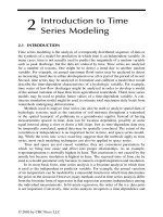
84 Mullins
Fig. 3 From left to right: Richards laboratory psychrometer with three sample cups

shown and nanovoltmeter attached; bottom left, field psychrometer sensor; portable meter
for puncture tensiometer; Webster (1966) tensiometer sensor; data logger with pressure
transducer. A porous ceramic tube and cup that can be attached to the transducer are shown
to the left; bottom center, filter paper ready to be placed on the soil in the plastic sample
container and covered with more soil.
Copyright © 2000 Marcel Dekker, Inc.
The discussion of methods so far has only considered designs that have been
used on disturbed soil samples in the laboratory. However, Spanner psychrometers
suitable for insertion into the soil for field or laboratory logging of water potential
are commercially available (Table 1, Figs. 3 and 4) and can be used in the dew
point or nonequilibrium mode. Psychrometers using all three principles of opera-
tion are commercially available for use in the laboratory with small (2 –15 cm
3
)
samples, although the nonequilibrium psychrometers may no longer be available.
Nanovoltmeters and automatic dew point control systems, made for use with psy-
chrometers, and systems that can automatically log a number of field psychrome-
ters, are also commercially available (Table 1). Wiebe et al. (1971) gave instruc-
tions for the construction of homemade psychrometers.
B. Limitations on Accuracy
All psychrometers are limited at the wet end of the range by the smallest tempera-
ture difference that can be meaningfully detected. Modern portable nanovolt-
meters have a readability of Ϯ 10 nV, corresponding to a potential of Ϯ 2kPa.
However, the problems associated with measuring such small temperature differ-
ences (ϳ0.0002ЊC) probably limit the useful range of current field psychrometers
to potentials below Ϫ100 kPa. The major factors that influence the accuracy of
psychrometer results and can cause large systematic errors are mainly associated
with temperature and diffusive error (Boyer, 1995). Temperature errors and how
to cope with them are shown in Table 2. A detailed review of the factors in this
table is given by Rawlins and Campbell (1986).

Precautions to minimize temperature gradients for laboratory bench psy-
chrometers include use in a room where temperature changes are not rapid
and there is little air movement, minimizing hand contact with the sample
changer, and encasing the sample changer in polyurethane foam or other thermal
Matric Potential 85
Fig. 4 Three-wire Spanner psychrometer (adapted from Rawlins and Campbell, 1986).
A stainless steel screen can be used in place of the porous cup.
Copyright © 2000 Marcel Dekker, Inc.
Table 2 Factors That Can Introduce Systematic Errors in Soil Psychrometer Readings
a
Factor and source Effect Remedy
1. Temperature gradients (variations in tempera-
ture of surroundings, electrical heating of
thermocouple wires, absorption of external
Temperature difference be-
tween reference and sensing
junction
i. (L) Use thermal insulation and/or a water bath to
avoid gradients, allow h for samples to equilibrate
1
2
in sample holder
radiation) ii. (Ps, Pd) If reference junction is isolated from sample,
measure temperature difference before Peltier cool-
ing and subtract it from the reading
iii. (F) Align psychrometer, with reference and sensing
junctions parallel to isotherms (i.e., insert parallel to
soil surface)
iv. (F) Use a thermally shielded psychrometer with
shield attached to reference junction

2. Temperature fluctuations with time As for 1 above As for 1 above
3. Variation in temperature of surroundings Variation in relative humidity
within chamber
Arrange sample to surround the sensing junction as
nearly as possible
4. Vapor pressure gradient (L) only (extraneous
sources or sinks of water vapor, especially
where samples are warmer than the chamber,
and water condenses on chamber walls)
Relative humidity in chamber
is not controlled by the
sample and reading is
erroneous
As for 3 above. Ensure that sample and holder have
reached the same temperature before moving under
the sensing junction; do not insert samples that are
warmer than the holder into it
5. Contamination of sensing junction or chamber
walls
Unreliable readings Clean junction and chamber and recalibrate
6. Zero offset Nonzero output when cali-
brated over water
Subtract offset reading before converting it to a potential
7. Temperature correction (calibration tem-
perature was not the same as measurement
temperature)
Not important for Pd; incorrect
readings for Pr and Ps
Calibrate at more than one temperature and interpolate
to measurement temperature or use a theoretical cor-

rection procedure
8. Insufficient equilibration (L) Incorrect reading Plot psychrometer reading versus time to gain famil-
iarity with its performance and use an adequate time.
Equilibration time reduced by remedy in 3 above
a
Key: L, laboratory sample changer arrangement; F, field psychrometer; Pr, Richards psychrometer; Ps, Spanner psychrometer; Pd, dew point mode.
Copyright © 2000 Marcel Dekker, Inc.
insulation. For samples with a high relative humidity (e.g. c
w
ϽϪ6 MPa),
samples should be transferred to and loaded into the sample changer in a humid
atmosphere (e.g., a box lined with wetted paper towels and with limited access,
ideally a glove box). Before measurement, samples should be kept in the same
room for at least 30 minutes to reach a similar temperature to the sample changer
and can require between 4 and 30 minutes within the sample changer for condi-
tions to approach vapor equilibrium (or steady state in a nonequilibrium psy-
chrometer). Suggested times are given in the manufacturer’s manuals and depend
on the apparatus and the magnitude of the potential being measured.
Use of laboratory apparatus on samples that have been taken from the field,
transported in sealed and thermally insulated containers, and then subsampled to
fill the sample holder, will depend on factors such as water loss by distillation onto
the container walls, variation of sample potential with temperature, and the effects
of mechanical disturbance on the measured potential.
C. Calibration and Solutions of Known Potential
Isopiestic psychrometers do not require calibration but do require solutions of
known potentials. Other psychrometers are usually calibrated by placing the sens-
ing junction over a range of salt solutions of known potentials in a constant-
temperature enclosure. Field psychrometers, for example, can be enclosed with
the solution in a sealed container in a water bath. There are published values of
the water potential of solutions of KCl (Campbell and Gardner, 1971), NaCl

(Lang, 1967), and sucrose (Boyer, 1995) at a range of temperatures. Details of
calibration of laboratory psychrometers are given in the manufacturer’s instruc-
tions. Merrill and Rawlins (1972) described calibration of field psychrometers,
and, for both laboratory and field psychrometers, recommended calibration pro-
cedures were given by Rawlins and Campbell (1986). If the sample temperature
is not the same as the temperature at which calibration was performed, and the
psychrometer is used in the nonequilibrium mode, it is necessary to make a tem-
perature correction. This can be done either by calibrating at a series of tempera-
tures and interpolation of the correct calibration curve or by a theoretical correc-
tion procedure (Merrill and Rawlins, 1972; Rawlins and Campbell, 1986).
D. Psychrometers for Insertion into the Soil
Only Spanner type psychrometers, which may be used in the dew point or non-
equilibrium mode, are available for field use. Figures 3 and 4 show a three-wire
psychrometer that includes a thermocouple to sense soil temperature. These are
particularly important for use in the nonequilibrium mode where temperature cor-
rection is required for accurate results (Merrill and Rawlins, 1972). Diurnal soil
temperature variations depend on climate. Their amplitude is considerably re-
duced by vegetation cover and decays exponentially with depth. They can impose
Matric Potential 87
Copyright © 2000 Marcel Dekker, Inc.
a serious limitation to the accuracy of psychrometer readings taken near to the soil
surface (Ͻ 0.25 m). Merrill and Rawlins (1972) have discussed the installation
and calibration stability of soil psychrometers. They observed errors of 50% for
Wescor ceramic-enclosed psychrometers installed vertically at a depth of 0.25 m
in soil with a bare surface. Diurnal temperature variation at this depth was
Ϯ 1.3Њ C, and when the psychrometers were installed horizontally to minimize
the influence of temperature gradients, the variation in readings was reduced to
ϳ 10%. Improved design can further reduce sensitivity to temperature gradients
(Bruini and Thurtell, 1982). In addition to horizontal placement, Merrill and Raw-
lins (1972) recommended that 50 –100 mm of the lead adjacent to the psychrome-

ter be horizontally oriented. They also observed a 5.3% median change in calibra-
tion sensitivity of 33 Wescor ceramic psychrometers after 8 months of field use;
only one psychrometer changed by Ͼ 15%. They considered that field psychrom-
eters were able to distinguish day-to-day changes in water potential to within
Ϯ 50 kPa.
There are two psychrometer versions that are commercially available, one
encased in a ceramic cup and one encased in a wire screen–shielded case (Fig. 3).
The ceramic cup excludes contamination by fungal hyphae and prevents flooding
of the chamber if it is below the water table for short periods. The screen-shielded
version should be more suitable in soils that are likely to shrink away from the
sensor during drying and may be less sensitive to temperature gradients (Merrill
and Rawlins, 1972).
E. Summary
For laboratory use, particularly as a standard against which to compare other tech-
niques, the isopiestic psychrometer is the most accurate but the most expensive
option, and a cheaper dew point hygrometer may have acceptable accuracy. Re-
sults obtained with a nonequilibrium psychrometer in optimal laboratory condi-
tions may also be useful where diffusive error can be minimized.
Field psychrometers are cheap and small but are limited in many situations
to use at Ͼ 0.25 m depth due to sensitivity to thermal gradients and are most
appropriate where measurement of low matric potentials (say ϽϪ300 kPa) are
required.
VI. APPLICATIONS
Measurement of soil matric, hydraulic, and water potentials are so fundamental
for studying water movement, germination, plant growth, and soil strength that
the literature is full of examples of the use of these measurements. Examples of
some of the major applications are given here.
88 Mullins
Copyright © 2000 Marcel Dekker, Inc.
Irrigation scheduling can be based on data from tensiometers (Hagan et al.,

1967; Cassell and Klute, 1986), electrical resistance (Goltz et al., 1981), or heat
dissipation sensors (Phene and Beale, 1976), all of which can be adapted to con-
tinuous logging and automatic irrigation control. Tensiometers, with their greater
accuracy but restricted lower limit, are most suitable for applications such as the
irrigation of vegetables and glasshouse crops, where it is intended to keep the soil
permanently at a high potential and where fairly accurate control is required to
avoid overwatering. Small portable tensiometers can be used for testing the suit-
ability of conditions for germination and establishment in seedbeds, peat blocks,
and other media used to raise plants (Goodman, 1983).
For monitoring the potential in the root zone under nonirrigated conditions,
the best accuracy will be obtained with a combination of tensiometers and either
psychrometers or heat dissipation sensors. If there is little recharge of the soil
profile during the growing season, it is possible to identify a zero flux plane, where
there is zero hydraulic potential gradient. This plane represents an imaginary wa-
tershed above which water moves upward to plant roots and below which drainage
may occur (McGowan, 1974; Arya et al., 1975; Cooper, 1980). By following the
movement of the zero flux plane down the profile during the growing season, it is
possible to follow changes in the maximum depth of root water extraction and to
obtain improved estimates of the soil water balance. Psychrometers designed for
attachment to leaves or stems (McBurney and Costigan, 1987) can be used in
combination with soil sensors to provide detailed information on the diurnal pat-
tern of the plant water regime (Bruini and Thurtell, 1982).
For measuring matric and hydraulic potential under wet conditions, there is
still no substitute for the accuracy of tensiometers, especially as they will function
equally well below the water table. Tensiometers can be used to study the water
regime in relation to restrictions on soil aeration and root growth (King et al.,
1986; Nisbet et al., 1989) and to follow the pattern of water flow that determines
the water regime on hillsides and in hollows (Anderson and Burt, 1977). Under
wet (C
m

ϾϪ10 kPa) conditions, portable tensiometers can be used to study spa-
tial variation of matric potential and hence the effectiveness of field drainage sys-
tems (Mullins et al., 1986).
Where data logging systems are too costly or impractical, the filter paper
technique has proved to be useful for studying temporal and spatial variations of
matric potential at remote sites, for example across gaps in the rainforest (Veenen-
daal et al., 1995). It is also useful for studying near-surface conditions such as in
seedbeds (Townend et al., 1996), where sensor size, response time, and tempera-
ture fluctuations limit the use of other techniques.
In addition to spatial variations resulting from plant water uptake, the soil
water regime may be heterogeneous in structured soils. Sensors that connect with
cracks or biopores, which form preferred pathways for infiltration, may then give
readings that differ from those installed within structural units. In such cases there
Matric Potential 89
Copyright © 2000 Marcel Dekker, Inc.