Soil and Environmental Analysis: Physical Methods - Chapter 6 pptx
Bạn đang xem bản rút gọn của tài liệu. Xem và tải ngay bản đầy đủ của tài liệu tại đây (685.01 KB, 42 trang )
6
Infiltration
Brent E. Clothier
HortResearch, Palmerston North, New Zealand
1. INTRODUCTION
A water droplet incident at the soil surface has just two options: it can infiltrate
the soil or it can run off. This partitioning process is critical. Infiltration, and its
complement runoff, are of interest to hydrologists who study runoff generation,
river flow, and groundwater recharge. The entry of water through the surface con-
cerns soil scientists, for infiltration replenishes the soil’s store of water. The par-
titioning process is critically dependent of the physical state of the surface. Fur-
thermore, infiltrating water acts as the vehicle for both nutrients and chemical
contaminants.
Infiltration, because it is both a key soil process and an important hydro-
logical mechanism, has been twice studied: once by soil physicists and again by
hydrologists. Historically, their approaches have been quite different. In the for-
mer case, infiltration was the prime focus of detailed study of small-scale soil
processes, and in the latter, infiltration was just one mechanism in a complicated
cascade of processes operating across the scale of a catchment. Latterly, access to
powerful computers has meant that hydrologists have been able to incorporate the
soil physicists’ detailed mechanistic descriptions of infiltration into their hydro-
logical models of watershed functioning. This has increased the need to measure
the parameters that control infiltration.
239
To the memory of John Philip (1927–1999), for without his endeavors this would have been a very
short chapter.
Copyright © 2000 Marcel Dekker, Inc.
In this chapter, I first describe the development of one-dimensional ponded
infiltration theory, discussing both analytical and quasi-analytical solutions. In
passing, I mention empirical descriptions of infiltration before discussing the key
development of a simple algebraic expression for infiltration that employs physi-
cally based parameters. Emphasis is placed on theoretical approaches, for they
can predict infiltration through having parameters capable of field measurement.
The preeminent roles of the physical state of the soil surface and the nature of the
upper boundary condition are stressed. Infiltration of water into soil can occur as
a result of there being a pond of free water on the soil surface, so that the soil
controls the amount infiltrated, or water can be supplied to the surface at a given
rate, say by rainfall, so the soil only controls the profile of wetting, not the amount
infiltrated.
Next, I show how measurement of infiltration can be used, in an inverse
sense, to determine the soil’s hydraulic properties. In this way, it is possible to
predict infiltration into the soil, and general prediction of water movement through
soil can also be made using these measured properties. Hydraulic interpretation of
the theoretical parameters in the governing equations is outlined, as is the impact
of infiltration on solute transport through soil. A list is presented of the various
devices that have been developed to measure, in the field, the soil’s capillary and
conductive properties that control infiltration. An outline of their respective merits
is presented, as is a comparative ranking of utility. Finally, I conclude with a pre-
sentation of some illustrative results and identify some issues that still remain
problematic.
Elsewhere in this book, there are complementary chapters on measurement
of the soil’s saturated conductivity (Chap. 4) and the unsaturated hydraulic con-
ductivity function (Chap. 5). Here the emphasis is on devices capable of in situ
observation of infiltration, and the measurement in the field of those saturated and
unsaturated properties that control the time course, and quantity, of infiltration.
II. THEORY
A. One-Dimensional Ponded Infiltration
Significant theoretical description of water flow through a porous medium began
in 1856 with Henry Darcy’s observations of saturated flow through a filter bed of
sand in Dijon, France (Philip, 1995). Darcy found that the rate of flow of water,
J (m s
Ϫ1
), through his saturated column of sand of length L (m), was proportional
to the difference in the hydrostatic head, H (m), between the upper water surface
and the outlet:
DH
J ϭ K (1)
ͩͪ
L
240 Clothier
Copyright © 2000 Marcel Dekker, Inc.
in which Darcy called K ‘‘un coefficient de´pendent du degre´ de perme´abilite´du
sable.’’ We now call this the saturated hydraulic conductivity K
s
(m s
Ϫ1
) (Chap. 4).
In 1907, Edgar Buckingham of the USDA Bureau of Soils established the theo-
retical basis of unsaturated soil water flow. He noted that the capillary conduc-
tance of water through soil, now known as the unsaturated hydraulic conductivity,
was a function of the soil’s water content, u (m
3
m
Ϫ3
), or the capillary pressure
head of water in the soil, h (m). The characteristic relationship between h and u
(Chap. 3) was also noted by Buckingham (1907), so that he could write K ϭ K(h),
or if so desired, K ϭ K(u). The total head of water at any point in the soil, H,is
the sum of the gravitational head due to its depth z below some datum, conve-
niently here taken as the soil surface, and the capillary pressure head of water in
the soil, h: H ϭ h Ϫ z. Here, h is a negative quantity in unsaturated soil, due to
the capillary attractiveness of water for the many nooks and crannies of the soil
pore system. Thus locally in the soil, Buckingham found that the flow of water
could be described by
dH dH
J ϭϪK(h) ϭϪK(h) ϩ K(h) (2)
ͩͪ
dz dz
which identifies the roles played by capillarity, the first term on the right hand
side, and gravity, the second term. These two forces combine to move water
through unsaturated soil (Chap. 5). In deference to the discoverers of the satu-
rated form, Eq. 1, and the unsaturated form, Eq. 2, the equation describing water
flow at any point in the soil is generally referred to as the Darcy–Buckingham
equation.
L. A. Richards (1931) combined the mass-balance expression that the tem-
poral change in the water content of the soil at any point is due to the local flux
divergence,
ץu ץJ
ϭϪ (3)
ͩͪ ͩͪ
ץt ץz
zt
with the Darcy–Buckingham description of the water flux J, to arrive at the gen-
eral equation of soil water flow,
ץu ץץhdK(h) ץh
ϭ K(h) Ϫ · (4)
ͩͪ
ץt ץz ץzdhץz
where t (s) is time. Unfortunately, this formula, known as Richards’ equation,
does not have a common dependent variable, for u appears on the left and h on
the right. The British physicist E. C. Childs ‘‘decided to try some other hypothe-
sis thatwatermovement is decided by the moisture concentration gradient . . .
[and] that water moves according to diffusion equations’’ (Childs, 1936). Childs
and Collis-George (1948) noted that the diffusion coefficient for water in soil
Infiltration 241
Copyright © 2000 Marcel Dekker, Inc.
could be written as K(u) dh/du. From this, in 1952 the American soil physicist
Arnold Klute wrote Richards’ equation in the diffusion form of
ץu ץץu dK ץu
ϭ D(u) Ϫ · (5)
ͩͪ
ץt ץz ץzdu ץz
This description shows soil water flow to be dependent on both the soil water
diffusivity function D(u), and the hydraulic conductivity function K(u), but this
nonlinear partial differential equation is of the Fokker–Planck form, which is no-
toriously difficult to solve. Klute (1952) developed a similarity solution to the
gravity-free form of Eq. 5, subject to ponding of free water at one end of a soil
column.
Five years later, the Australian John Philip developed a power-series solu-
tion to the full form of Eq. (5), subject to the ponding of water at the surface of
a vertical column of soil, initially at some low water content u
n
(Philip, 1957a).
This general solution predicts the rate of water entry through the soil surface, i(t)
(m s
Ϫ1
), following ponding on the surface. The surface water content is main-
tained at its saturated value, u
s
. The cumulative amount of water infiltrated is
I (m), being the integral of the rate of infiltration since ponding was established.
As well, I can be found from the changing water content profile in the soil,
t ϱ u
s
I ϭ ͵ i(tЈ) dtЈ ϭ ͵ u(zЈ) Ϫ u dzЈ ϭ ͵ z(u) du (6)
ͫͬ
n
00 u
n
Philip’s (1957a) series solution for I(t) can be written
1/2 3/2 4/2
···
I(t) ϭ St ϩ At ϩ At ϩ At ϩ (7)
34
where the sorptivity S (m s
Ϫ1/2
) and the coefficients A, A
3
, A
4
, canbeitera-
tively calculated from the diffusivity and conductivity functions, D(u) and K(u).
The form of Eq. 7 indicates that I increases with time, but at an ever-decreasing
rate. In other words, the rate of infiltration i ϭ dI/dt is high initially, due to the
capillary pull of the dry soil. But with time the rate declines to an asymptote.
Special analytical solutions can be found for cases where certain assump-
tions are made about the soil’s hydraulic properties. When the soil water diffusiv-
ity can be considered to be a constant, and K varies linearly with u, an analytical
solution is possible. This is because Eq. 5 becomes linearized (Philip, 1969) and
so there is an analytical solution for infiltration into a soil whose hydraulic prop-
erties can be considered only weakly dependent on u. At the other end of the scale
of possible behavior, Philip (1969) presented an analytical solution for a soil
whose diffusivity could be considered a Dirac d-function, in which D is zero,
except at u
s
where it goes to infinity. For the analytical solution, this so-called
delta-soil, or Green and Ampt soil, also needs to have K ϭ K
s
at u
s
, and K ϭ 0 for
all other u.
242 Clothier
Copyright © 2000 Marcel Dekker, Inc.
Philip and Knight (1974) showed that the Dirac d-function solution pro-
duces a rectangular profile of wetting (shown later in Fig. 4). It was this geometric
form of wetting that was used as the physical basis for Green and Ampt’s (1911)
functional model of infiltration. If a rectangular profile of wetting is assumed, then
behind the wetting front located at depth z
f
, u(z) ϭ u
s
, for 0 Ͻ z Ͻ z
f
; and beyond
the wetting front, u(z) ϭ u
n
, z Ͼ z
f
. If the soil has a shallow free-water pond at
the surface, and if it is considered that there is a wetting front potential head, h
f
,
at z
f
, then the Darcy–Buckingham law (Eq. 2) predicts the rate of water infiltrat-
ing through the surface as
K (z Ϫ h )
sf f
J ϭ (8)
z
f
The rectangular profile of wetting allows easy evaluation of the mass balance
integral of Eq. 6, and its differentiation to provide the rate of infiltration into
the soil,
dI d(z (u Ϫ u )) dz
fs n f
i ϭϭ ϭ ·(u Ϫ u ) (9)
sn
dt dt dt
Equating Eqs. 8 and 9 provides a variables-separable ordinary differential equa-
tion in z
f
,
(z Ϫ h ) dz
ff f
K ϭ (u Ϫ u ) (10)
ssn
zdt
f
which can be solved to provide the penetration of the wetting front into the soil
with time,
(u Ϫ u ) z
sn f
t ϭ z ϩ h ln 1 Ϫ (11)
ͫͩͪͬ
ff
Kh
sf
Althrough this expression is not explicit, it does allow implicit prediction of I(t)
from basic soil properties. By considering flow in the absence of gravity, z
f
is
eliminated from the numerator of Eq. 8, and an explicit expression for gravity-free
infiltration is arrived at that only contains a square-root-of-time term, as would be
expected for a diffusion-like process. By comparing coefficients with Eq. 7, it is
found that a Green and Ampt soil must have the sorptivity
2
S ϭϪ2Kh(u Ϫ u ) (12)
sf s n
So, if the soil is considered to have the characteristics that lead to a rectangular
profile of wetting (shown in Fig. 4), and there is a constant pressure-potential
head, h
f
, always associated with the wetting front, then simple expressions can be
derived to predict infiltration into such a soil (Eqs. 11 and 12).
More recently, Parlange (1971) developed a new and general quasi-analyti-
cal solution for infiltration into any soil (Eq. 5). This was extended by Philip and
Infiltration 243
Copyright © 2000 Marcel Dekker, Inc.
Knight (1974) using a flux– concentration relationship, F(Ѳ), that hides much of
the nonlinearity in the soil’s hydraulic properties of D and K. Here Ѳ is the nor-
malized water content.
Considering these mathematical solutions to the flow equation for infiltra-
tion I, subject to ponding, Childs (1967) commented that ‘‘further investigations
to throw yet more light on the basic principles of the flow of water tendtobe
matters of crossing t’s and dotting i’s . . . serious difficulties remain in the path of
practical application of theory . . . [being] held back by the inadequate develop-
ment of methods of assessment of the relevant parameters.’’
These analytical or quasi-analytical solutions are seldom used to predict
infiltration directly from the soil’s hydraulic properties. The theory and its de-
velopment are presented here, for they identify the underpinning physics of infil-
tration. Nowadays, however, the current power of computers, coupled with the
burgeoning growth of numerical recipes for solving nonlinear partial differen-
tial equations, has meant that brute-force numerical solutions to Eq. 5 for infil-
tration are easily obtained, provided that the functional properties of D and K
are known. Thus given a knowledge of the soil’s hydraulic properties, it is a
reasonably straightforward exercise to predict infiltration, either analytically or
numerically.
Infiltration measurements hold the key to obtaining in situ characterization
of these soil properties. It is possible to use Eq. 7 or the like in an inverse sense,
to use infiltration observations to infer the soil’s hydraulic character. The time
course of water entry into soil, I(t), depends, as Eq. 7 shows, on coefficients that
relate to the hydraulic properties of D(u) and K(u). Infiltration can quite easily be
measured in the field. Hence, I will proceed to show how this measurement of I
can be used to extract in situ information about the soil’s capillary and conductive
properties.
1. Empirical Descriptions
Before passing to the discussion of the developments that have led to the use of
measurements to predict one-dimensional infiltration behavior, I sidetrack a little
to review some of the empirical descriptions of the shape of i(t). This digression
is simply to complete our historical record of the study of infiltration, for such
empirical equations have little merit nowadays. The Kostiakov–Lewis equation,
I ϭ at
b
(Swartzendruber, 1993), has descriptive merit through its simplicity, yet
comparison with Eq. 7 indicates the inadequacy of this power-law form, for in
reality b needs to be a function of time. The hydrologist Horton (1940) pro-
posed that the decline in the infiltration rate could be described using i ϭ i
ϱ
ϩ
(i
o
Ϫ i
ϱ
) exp(Ϫbt), where the subscripts o and ϱ refer to the initial and final rates.
If description is all that is sought, then the three-term expression will perform
better due to its greater fitting ‘‘flexibility.’’ In neither case do the fitted parameters
244 Clothier
Copyright © 2000 Marcel Dekker, Inc.
have physical meaning, so care needs to be exercised in their extrapolation beyond
the fitted range.
2. Physically Based Descriptions
However, the two-term algebraic equation of Philip (1957b) is different from other
empirical descriptions. It rationally incorporates physical notions. Simply by trun-
cating the power series of Eq. 7, Philip (1957a) arrived at the expression for the
infiltration rate of
1
Ϫ1/2
i ϭ St ϩ A (13)
2
which will be applicable at short and intermediate times. However at longer times,
we know for ponded infiltration that
lim i(t) ϭ K (14)
s
→
t ϱ
The means by which these two expressions can best be joined has worried some
soil physicists, with A/K
s
having been found to be bracketed between 1 Ϫ 2/p
and 2/3, but probably lying nearer the lower limit (Philip, 1988). However, as
Philip (1987) noted, relative to practical incertitudes, a two-term algebraic expres-
sion often suffices, with both terms having physical meaning, plus correct short-
and long-time behavior, viz.
1
Ϫ1/2
i ϭ St ϩ K (15)
s
2
The coefficient of the square-root-of-time term, the sorptivity S, integrates the
capillary attractiveness of the soil. Mathematically, as we will see later, this can
be linked to the soil water diffusivity function D(u). The role of capillarity de-
clines with the square root of time. The second term, which is time independent,
is the saturated conductivity K
s
, which is the maximum value of the conductivity
function K(h) that occurs when the soil is saturated, h ϭ 0. If the soil is initially
saturated (S ϭ 0), or if infiltration has been going on for a long time, then gravity
will alone be drawing water into the soil at the steady rate of K
s
. Eq. 15 is aptly
named Philip’s equation.
To understand Eq. 15 is to understand the basics of infiltration.
B. Multidimensional Ponded Infiltration
However, a one-dimensional geometric description is not always appropriate. For
example, infiltration into soil might be from a buried and leaking pipe, or it might
be from a finite surface puddle of water. In these cases, the physics previously
Infiltration 245
Copyright © 2000 Marcel Dekker, Inc.
described above must now be referenced to the geometry of the source. The re-
spective roles of capillarity and gravity in establishing the rate of multidimen-
sional infiltration, v
o
(t)(ms
Ϫ1
), through a surface of radius of curvature r
o
(m),
are now more complex. Following Philip (1966), let m be the number of spatial
dimensions required for geometric description of the flow. The geometry depicted
in Fig. 1 might be a transverse section through a cylindrical channel. This would
be a 2-D source with m ϭ 2. Or it could be a diametric cut through a spherical
pond that would be represent a 3-D geometry. So here m ϭ 3. The more curved
the wetted perimeter of the source, the smaller is r
o
, and the greater is the role of
the soil’s capillarity relative to gravity. In the limit as r
o
→ ϱ, the geometry be-
comes one-dimensional (m ϭ 1), and the source spreads right across the soil’s
surface.
As already noted, if the soil is considered to have a constant diffusivity D,
and a linear K(u), then ananalytical solution can be found for one-dimensional
infiltration because the governing equation is linearized. This also applies to
multidimensional infiltration, if the flow description of Eq. 5, which has m ϭ 1,
is written in a form appropriate to a flow geometry with either m ϭ 2orm ϭ 3
(Philip, 1966). Philip’s (1966) linearized multidimensional infiltration results are
illustrative and are presented in Fig. 2. There, the infiltration rate through the
wetted perimeter, v
o
, is normalized with respect to the saturated conductivity K
s
,
and the time is normalized by a nondimensional time, t
grav
ϭ (S/K
s
)
2
. To allow
246 Clothier
Fig. 1. An idealized multidimensional infiltration source, in which water infiltrates into
the soil through a wetter perimeter of radius of curvature r
o
. Capillarity and gravity com-
bine to draw water into the dry soil.
Copyright © 2000 Marcel Dekker, Inc.
easy comparison, the radius of curvature is also normalized, and given as R
o
ϭ
r
o
[K
s
(u
s
Ϫ u
n
)
2
/pS
2
].
For the one-dimensional case in Fig. 2 (m ϭ 1), the infiltration rate can be
seen to fall, as the effects of capillarity fade with the square, and higher, roots of
time (Eq. 7). At around t/pt
grav
, the infiltration rate is virtually the asymptote of
v
o
ϭ K
s
. Such behavior is predicted by Eq. 15. Two cases are given for two-
dimensional flow from cylindrical channels, m ϭ 2. For the tightly curved channel
(R
o
ϭ 0.05), the effect of the source geometry on capillarity is clearly seen, and
the infiltration rate is nearly two times K
s
at dimensionless time 10. For the less-
curved channel (R
o
ϭ 0.25), the geometry-induced enhancement of capillary ef-
fects is correspondingly less. In the three-dimensional case (m ϭ 3), for the curved
spherical pond with R
o
ϭ 0.05, the effect of capillarity is so enhanced by the 3-D
source geometry that the infiltration rate through the pond walls achieves a steady
flux of over 5K
s
by unit time.
Whereas infiltration in one dimension (m ϭ 1) gradually approaches K
s
,the
source geometry in 2-D and 3-D (m ϭ 2 and 3) ensures that the infiltration rate
finally arrives at a true steady-state value, v
ϱ
. In Fig. 2, the time taken to realise v
ϱ
Infiltration 247
Fig. 2. The normalized temporal decline in the rate of infiltration through the ponded
surface into a one-dimensional soil profile (m ϭ 1), and from two cylindrical channels
(m ϭ 2) of contrasting radii of curvature (r
o
), as well as from two spherical ponds (m ϭ 3)
of different radii. To allow comparison of one-, two-, and three-dimensional flows, the
infiltration rate, time, and radii of source curvature have all been normalized. (Redrawn
from Philip, 1966.)
Copyright © 2000 Marcel Dekker, Inc.
is more rapid in 3-D than it is for m ϭ 2. This achievement of a steady flow rate
in 3-D is, as we will see later, a major advantage for certain devices in the field
measurement of infiltration.
In this device-context, it is useful to consider in more detail the three-
dimensional flow from a shallow, circular pond of water of radius r
o
. The history
of the study of this problem is given in Clothier et al. (1995), so here we need only
concern ourselves with the seminal result of Wooding (1968). The New Zealander
Robin Wooding was concerned about the radius requirements for double-ring in-
filtrometers (shown later in Fig. 5), and he found a complex-series solution for the
steady flow from a shallow, circular surface pond of free water. However, he did
note that the steady flow could be approximated by a simple equation in which
capillary effects were added to the gravitational flow in inverse proportion to the
length of the wetted perimeter of the pond,
4f
s
v ϭ K ϩ (16)
ϱ s
pr
o
Here the sum effect of the soil’s capillarity is expressed in terms of the integrals
of the hydraulic properties of D and K, the so-called matric flux potential
u 0
s
f ϭ ͵ D(u)du ϭ ͵ K(h)dh (17)
s
u h
n
It was necessary for Wooding (1968) to consider that the soil’s unsaturated hy-
draulic conductivity function could be given by the exponential form
K(h) ϭ K exp(ah) (18)
s
with the unsaturated slope a (m
Ϫ1
), so that
K
s
f ϭ (19)
s
a
This formulation allows Wooding’s equation (Eq. 16) for the steady volumetric
infiltration from the circular pond, Q
ϱ
ϭ pr
o
2
v
ϱ
(m
3
s
Ϫ1
), to be written as
4r
o
2
Q ϭ K pr ϩ (20)
ͩͪ
ϱ so
a
In this way we can see the role of the pond’s area in generating the gravitational
component of infiltration, and that of the perimeter in creating a capillary contri-
bution. We will return later to this special form of multidimensional ponded
infiltration.
C. Boundary Conditions
Thus far, we have only considered the case where water is supplied by a surface
pond of free water, namely
248 Clothier
Copyright © 2000 Marcel Dekker, Inc.
u(0, t) ϭ u h(0, t) ϭ 0 z ϭ 0, t Ն 0 (21)
s
This is termed a constant-concentration boundary condition and known mathe-
matically as a first-type or Dirichlet boundary condition. This is appropriate to
cases where water is ponded on the ponded on the soil surface. The soil’s hydraulic
properties, and source geometry, determine the rate and temporal decline in infil-
tration (Fig. 2). The water content at the soil’s surface is always at its saturated
value, u
s
.
However, often water arrives at the soil surface as a flux, as might occur
during rainfall, or irrigation. In this case, the upper boundary condition is the
applied flux v
o
,
ץu ץH
D(u) ϭ K(h) ϭϪvzϭ 0, t Ն 0 (22)
o
ץz ץz
This case is mathematically termed a second type or Neumann boundary condi-
tion, and the amount and rate of water infiltrating the soil is independent of the
soil’s hydraulic properties. Rather, it is determined by v
o
. Whereas in Eq. 21 the
water content at the soil surface is constant, under a flux condition, as the soil
wets, the water content at the surface, u
o
, rises: u
o
ϭ u
o
(t).
Should the flux of water always be less than K
s
, then the water content at
the surface will always be less than u
s
. The soil at the surface will remain unsatu-
rated, h
o
Ͻ 0, and all the incident water will enter the soil, with I ϭ v
o
t.
However, if the rate of water falling on the soil surface exceeds K
s
, then
eventually at some time t
p
, the time to incipient ponding, the soil at the surface
will saturate; h
o
ϭ 0; u
o
ϭ u
s
, t Ն t
p
. After this incipient ponding, runoff from
the free water pond can occur, and not all the applied water need enter the soil:
I Ͻ v
o
t, for t Ն t
p
. For the case of a constant flux, Perroux et al. (1981) found that
a good approximation for the time to ponding was
2
S
t ϭ (23)
p
2v (v Ϫ K )
oo s
So the greater the flux the quicker the soil surface ponds. Conversely, the drier the
soil initially, the greater is the capillarity of the soil, the higher is S, and so the
longer can the soil maintain its acceptance of all the applied water.
The presence or absence of a surface pond of free water is critical for infil-
tration behavior in the macropore-ridden soils of the field. This is shown in Fig. 3.
Only free water (h
o
Ͼ 0) can enter surface-vented macropores. Thus during non-
ponding flux infiltration, v
o
Ͻ K
s
, or prior to the time to ponding, t Ͻ t
p
, the soil
surface remains unsaturated, h
o
Ͻ 0, so that water does not enter macropores.
Rather the water droplets are absorbed right where they land. Hence the pattern of
infiltration and soil wetting is quite uniform, as capillarity attempts to even out
local heterogeneities. However, following incipient ponding, t Ͼ t
p
, a free-water
film develops on the soil surface. This free water can enter surface-vented macro-
Infiltration 249
Copyright © 2000 Marcel Dekker, Inc.
pores, creating preferential flow through the soil, and lead to local variability in
the pattern of soil wetting. If the infiltration capacity of the soil, both by matrix
absorption and macropore flow, is exceeded, there is the possibility of local runoff
once the surface storage has been overwhelmed (Dixon and Peterson, 1971).
The magnitude of the flux v
o
relative to the soil’s K
s
is critical in determining
infiltration behavior, and during flux infiltration it is critical to know whether the
time to ponding has been reached. The value of t
p
can be deduced from a knowl-
edge of the soil’s sorptivity S, and conductivity K
s
,givenv
o
(Eq. 23). So it is
imperative that S and K
s
be measured for field soils.
D. Hydraulic Characteristics of Soil
There are three functional properties necessary to describe completely the hydrau-
lic character of the soil: the soil water diffusivity function D(u), the unsaturated
hydraulic conductivity function K(h), and the soil water characteristic u(h). How-
ever since D ϭ Kdh/du, only two are sufficient to parameterize Eq. 5. Whereas it
is possible to measure these functions in the laboratory, albeit with some difficulty,
it is virtually impossible to do so in the field (Chaps. 3 and 5).
Nonetheless, if we were to observe the time course of ponded infiltration in
the field, i(t), then by inverse procedures we should be able to use Eq. 15 to infer
values of the saturated sorptivity S, and the saturated conductivity K
s
. In the first
case, we would then have obtained a measurement of something that integrates
250 Clothier
Fig. 3. Infiltration of an applied flux of water into soil. Left: non-ponding infiltration
when v
o
Ͻ K
s
, or ponding infiltration v
o
Ͼ K
s
prior to the time to ponding t
p
. Right: pattern
of infiltration after incipient ponding, t Ͼ t
p
, when the possibility of runoff exists, as does
the entry of free water into macropores.
Copyright © 2000 Marcel Dekker, Inc.
the soil’s capillarity, and in the second case we would know the maximum value
of the K(h) function. Because we know in one case an integral measure, and in the
other a functional maximum, if we were willing to make some assumptions about
functional forms, we could infer the D andK functions from measurements of just
S and K
s
, and some observations of u
s
and u
n
. Thus observations of infiltration in
the field can be used to establish the hydraulic characteristics of field soil.
Formally, the sorptivity can be written as a complicated integral of the soil
water diffusivity function
u
s
(u Ϫ u ) D(u)
n
2
S (u , u ) ϭ 2͵ du (24)
sn
u
F(Ѳ)
n
where F is the flux– concentration relation of the quasi-analytical solution of
Philip and Knight (1974) (see Sec. II.A). Parlange (1975) independently found
some useful and simple algebraic versions of Eq. 24. Eq. 24 is difficult to invert
in order that D(u) might be deduced from S. However, if we revisit the Kirchhoff
transform of Eq. 17, we have the integral of the diffusivity as
u
s
f ϭ ͵ D(u) du (25)
s
u
n
so that by inspection of Eqs. 24 and 25, we would expect a relationship between
f
s
and S
2
. White and Sully (1987) wrote this as
2
bS
f ϭ (26)
s
u Ϫ u
sn
where it is known theoretically that Ͻ b Ͻ p/4. For a wide range of soils they
1
2
found b ϭ 0.55 to be a robust assumption. Thus from a measurement of the sorp-
tivity, we can infer the integral of the diffusivity function f
s
. If we were willing to
make some assumption about the form of D(u), say an exponential with slope 8
(Brutsaert, 1979), then by measuring S, u
s
, and u
n
, and using Eq. 26, we would
be able to realize a functional representation of the soil water diffusivity that is
capable of parameterization in the field (Clothier and White, 1981). At least, it
would be integrally correct.
If we look yet again at Eq. 17, we see that f
s
is also the integral of the K(h)
function. If an exponential conductivity function (Eq. 18) is assumed, then
0
K
s
f ϭ ͵ K(h) dh ϭ (27)
s
h
a
This can be combined with Eq. 26 to obtain the slope,
KK(u Ϫ u )
sssn
a ϭϭ (28)
2
f bS
s
Infiltration 251
Copyright © 2000 Marcel Dekker, Inc.
So by monitoring infiltration to infer both K
s
and S (Eq. 15), and by measuring u
s
and u
n
, Eqs. 26 and 28 give us functional descriptions of the soil’s D(u) and K(h).
These capillary and gravity properties allow us to infer some pore-geo-
metric characteristics of the soil’s hydraulic functioning. Philip (1958) defined a
macroscopic, mean ‘‘capillary length’’ l
c
, which can be written over the range
from h
n
to saturation as
0 u
s
͐ K(h) dh ͐ D(u) du
h u
nn
l ϭϭ (29)
c
KK
ss
if the conductivity at h
n
is considered to be negligible. This corresponds to the
capillary fringe of Myers and van Bavel (1963), and the critical pressure of Bou-
wer (1964). Note that if the soil’s K(h) is exponential (Eq. 18), then Eq. 27 shows
us that l
c
ϭ a
Ϫ1
. Using Eq. 28 gives l
c
in terms of easily measurable quantities,
2
bS
l ϭ (30)
c
K (u Ϫ u )
ss n
Using Laplace’s capillary-rise formula, Philip (1987) related l
c
to the character-
istic mean pore radius, l
m
:
s 17.4
l ϭ ഠ (31)
m
rg ll
cc
if appropriate values are taken for the surface tension s and density r of water,
and for the acceleration due to gravity. White and Sully (1987) called l
m
a ‘‘physi-
cally plausible estimate of flow-weighted mean pore dimensions.’’ By combining
Eqs. 30 and 31 it is possible to use properties measured during infiltration (S and
K
s
; u
s
and u
n
) to deduce something dynamic about the magnitude of the pore size
class involved in drawing water into the soil. Namely,
13.5(u Ϫ u )K
sns
l ϭ (32)
m
2
S
E. Solute Transport During Infiltration
Water is the vehicle for solutes in soil. Here, for simplicity, we consider a soil
lying horizontally with water being absorbed in the x direction. During infiltration,
water-borne chemicals are transported into the soil. The entry of water into soil is
a hydrodynamic phenomenon: the wetting front rides into the soil on ‘‘top’’ of the
antecedent water content, u
n
(Fig. 4). For the case of a d-function soil, that is, one
possessing Green and Ampt’s (1911) rectangular profile of wetting, Eq. 6 gives
the penetration of the wetting front as
252 Clothier
Copyright © 2000 Marcel Dekker, Inc.
I
x ϭ (33)
f
(u Ϫ u )
sn
The transport of water-borne solute, during this hydrodynamically driven infiltra-
tion process, is an invasion mechanism. If all the soil’s water is mobile, and if
dispersion is ignored, then the invading solute profile will also be rectangular
(Fig. 4). In this case, the solute front will be at
I
s ϭ (34)
f
u
s
For field soils, due to preferential flow paths, it has been found useful to treat
chemical invasion as if not all of the soil’s water is mobile. As an approximation,
the soil’s water can be conveniently partitioned into a mobile phase, u
m
, and a
complementary domain that is considered effectively immobile, u
im
; u
s
ϭ u
m
ϩ
u
im
(van Genuchten and Wierenga, 1976). In this mobile-immobile case, the solute
front would be further ahead at
I
s ϭ (35)
f
u
m
because u
m
Ͻ u
s
. Thus if some inert tracer solution were allowed to infiltrate
the soil, then the position of the wetting front, relative to that of the solute front,
would be
x u
fm
ᑬ ϭϭ (36)
s u Ϫ u
fsn
Infiltration 253
Fig. 4. Left: rectangular profile of wetting that pertains during infiltration into a soil
whose diffusivity function is a Dirac d-function (Green and Ampt, 1911). The position of
the wetting front x
f
is given by Eq. 33. Right: a dispersion-free invasion front of the solution
infiltrating a soil in which all the water is assumed to be mobile, and one in which the
mobile water content is just u
m
. The solute fronts for these two cases, s
f
, are given by
Eq. 34.
Copyright © 2000 Marcel Dekker, Inc.
So in a fully mobile case u
m
ϭ u
s
, which is initially dry, u
n
ϭ 0, the wetting front
and the invading inert solute front will be coincident; ᑬ ϭ 1. If the soil is not
initially dry, then the wetting front will be ahead of the invasion front of the solute,
ᑬ Ͼ 1. If not all the soil’s water is mobile, then the solute will preferentially
infiltrate the soil through just the mobile domain, and the solute front may be
closer to the wetting front. The simple notions contained in Fig. 4 and Eq. 35
provide a useful means to model chemical transport processes during infiltration.
Later, I will discuss how values of u
m
and ᑬ might be measured and interpreted.
III. DEVICES AND MEASUREMENT
In this section, I now consider eight devices that have been developed to measure
infiltration in the field. The relative merits of these devices and instruments are
listed in Table 1 and discussed later.
A. Rings
1. Buffered Rings
The easiest way to observe ponded infiltration in the field is simply to watch the
rate that water disappears from a surface puddle. However, as shown in Fig. 1,
two factors control infiltration from a pond, capillarity and gravity. In order to
eliminate the perimeter effects of capillarity, buffered rings have been used so that
the flow in the inner ring is due only to gravity (Fig. 5). By this arrangement, it is
hoped that the steady flux from the inner ring, v
ϱ
, might be the saturated hydraulic
conductivity K
s
, since capillary effects would be quenched by flow from the buffer
ring, v
o
*. To determine what size the radius of the inner ring, r
1
, needs to be
relative to that of the buffer, r
2
, Bouwer (1961) and Youngs (1972) used an elec-
trical-analog approach, whereas Wooding (1968) provided a simple expression
based on the properties of the soil (Eq. 16). The ASTM standard double-ring in-
filtrometer has radii of 150 and 300 mm (Lukens, 1981), although the correct ratio
will be soil dependent, and related to the relative sizes of the conductivity K and
the sorptivity S (Eq. 16). The flows v
o
and v
o
* can be measured using a Mariotte
supply system that maintains a constant head within the rings (Constantz, 1983).
Or more simply, a nail can be pushed into the soil, and a measuring cylinder used
to top-up the water level to it at regular intervals. This approach may require a
large amount of water, especially if the soil is dry and has a high S, such that in
the buffer ring v
o
* is large. From the measured steady flux it is assumed that v
ϱ
ϭ
K
s
. The role of the buffer ring is to eliminate capillary effects, so this method
provides only the saturated hydraulic conductivity and leaves unresolved any mea-
sure of the soil’s capillarity.
254 Clothier
Copyright © 2000 Marcel Dekker, Inc.
Table 1 The relative merits of field infiltration devices against a set of criteria where the ranking of 5 implies cheap, easy, or high, and
1 suggests expensive, difficult, or low. Each attribute column contains at least one 5 (top) and at least one 1 (worst). The overall Utility of each
device was found as the sum of the first six columns, multiplied by the Information content. A high Utility score indicates usefulness, with the
maximum range possible being from 150 down to 6
Device
Cost
5 ഠ US$100
1 ഠ US$10,000
Physical
ease of
field use
Technical
skills
required
Site
disturbance
Ease of
data
analysis
Ease of
time–space
replication
Information
content Utility score
Rings 555154375
Wells, auger hole
permeameters 2 3 3 2 3 4 4 68
Pressure
infiltrometers 2 2 2 1 3 4 3 42
Closed-top
permeameters 2 2 1 1 1 1 2 16
Crust test 3 2 2 3 2 1 3 39
Tension and disc
infiltrometers 2 3 2 4 2 4 5 85
Drippers 3 2 2 5 2 5 3 57
Rainfall simulators 1 1 1 5 3 1 1 12
Copyright © 2000 Marcel Dekker, Inc.
2. Single Ring
If a single ring were forced into the soil to some depth, L, then that ring would
confine the flow to the vertical and thereby eliminate the multidimensional con-
fusion created by capillarity. Talsma (1969) developed a method whereby it is
possible to measure both the sorptivity and the conductivity. A metal ring of a
diameter about 300 mm and length L of around 250 mm is pressed into the soil so
as to minimize the disturbance of the soil’s structure. A free-board of about 50 mm
is left, and a graduated scale is laid diametrically across the ring, with one end on
the rim and the other on the soil surface. The slope of the scale is measured. A
fixed volume of water is then carefully poured into the ring, and the early-time
rate of infiltration is obtained from the descent of the water surface along the
sloping scale. At very short times, soon after infiltration commences and before
gravitational effects intercede, it is reasonable to assume that the integral form of
Eq. 15 can be written as
1/2
lim I ϭ St (37)
→
t0
so that the sorptivity can be found as the slope of I(͌t). Because gravity’s impact
grows slowly, it can be difficult to select the length of period within which to fit
Eq. 37. Smiles and Knight (1976) found that plotting (It
Ϫ1/2
) against ͌t allowed
a more robust means of extracting S from the cumulative infiltration data.
256 Clothier
Fig. 5. Infiltration into soil from two concentric rings pressed gently into the soil. The
flow in the outer ring of radius r
2
,isv
o
*, and this is presumed to eliminate perimetric
capillary effects so that the steady flux in the inner ring v
ϱ
can be considered K
s
.
After the initial wetting, typically after about 10 to 15 minutes, Talsma’s
method requires that the ring containing the soil be exhumed and placed on a fine-
mesh metal grid. A Mariotte device is then used to maintain a small head of water,
Copyright © 2000 Marcel Dekker, Inc.
h
o
, on the surface of the soil. Once water is dripping out the bottom, the steady
flow rate J can be measured, and Darcy’s law (Eq. 1) used to find the saturated
hydraulic conductivity K
s
.
This simple and inexpensive method allows measurement of both the soil’s
capillarity via S and the saturated conductivity of K
s
. However, extreme care has
to be taken to minimize the disturbance of the soil during insertion. In macropo-
rous soil this will be difficult, and furthermore any macropores that are continuous
through the entire core will short-circuit the matrix and result in an erroneously
high value of K
s
.
3. Twin Rings
With the buffered-ring system, capillarity effects are hopefully eliminated. With
the single-ring technique, hopefully the effects due to capillarity are measured
before those of gravity intervene. But in the twin-ring method of Scotter et al.
(1982), two separate rings of different size are used to exploit the dependence of
capillarity on the radius of curvature of the wetted source (Fig. 1). The capillary
and gravitational influences on infiltration can be separated (Youngs, 1972). Two
rings of different diameters are used, and these are simply pressed lightly into the
soil surface. A constant head of water is maintained inside both rings, so that the
unconfined steady 3-D flow (Figs. 1 and 2) can be measured: v
1
for the smaller
ring of radius r
1
, and v
2
for the larger ring of r
2
. The flux density of flow from the
smaller ring will be higher than that of the larger ring by an amount that will reflect
the soil’s capillarity, namely its sorptivity (Figs. 1 and 2). Substituting r
1
and r
2
into Eq. 16 gives simultaneous equations that can be resolved to find the conduc-
tivity as
vr Ϫ vr
11 22
K ϭ (38)
s
r Ϫ r
12
and the matric flux potential as
p v Ϫ v
12
f ϭ · (39)
ͩͪ
s
41/r Ϫ 1/r
12
From f
s
it is possible to obtain the sorptivity S (Eq. 26), as long as u
n
and u
s
are
measured before and after infiltration. In practice, replicates are taken so that the
mean values of and are used in Eqs. 38 and 39. Scotter et al. (1982) showedvv
{ {
12
how the variance in S and K
s
can be calculated.
This twin-ring technique allows both the soil’s capillarity and its conductiv-
ity to be measured, and here the disturbance to the soil’s structure is minimal. It is
only necessary to press the rings gently into the soil surface, and a mud caulking
can be used to seal the ring to the surface. The technique requires, however, that
there be a significant difference in the fluxes between rings, and this is dependent
Infiltration 257
Copyright © 2000 Marcel Dekker, Inc.
upon the relative sizes of the soil’s capillarity and conductivity (Figs. 1 and 2).
Scotter et al. (1982) showed that these effects are equal when a ring of radius r
e
ϭ
4f
s
/pK
s
is used. Larger rings are required to obtain an estimate of the K
s
of finer-
textured soils, and small rings are required to obtain a good estimate of the f
s
of
coarse-textured soils. Scotter et al. (1982) thought rings of r ϭ 0.025 and 0.5 m
would be suitable for a wide range of soils. If the difference in the radii is not large
enough, or if there are too few replicates to obtain a reliable estimate of the v ’s,
{
erroneous values will result (Cook and Broeren, 1994).
B. Wells and Auger Holes
1. Glover’s Solution
It has long been known that water flow from a small surface well soon attains a
steady rate, Q (m
3
s
Ϫ1
), and that in some way this flux is related to the soil’s
hydraulic character, the depth of water in the hole, H, and its radius, a (Fig. 6).
If capillarity is ignored, and if it can be considered that the surrounding soil is
wet and draining at the rate of K
s
, then it is the pressure head H that generates the
flow Q. Glover (1953) found that the soil’s hydraulic conductivity could thus be
found as
CQ
K ϭ (40)
s
2
2pH
where the geometric factor C is given by
2
Ha a
Ϫ1
C ϭ sinh Ϫϩ1 ϩ (41)
ͩͪ
Ί
aH H
Thus simply by creating a small auger hole of radius a, and using a Mariotte
device to maintain a constant head H, it is possible to use Q to infer the soil’s
saturated conductivity, K
s
. Holes with a ഡ 20 –50 mm and H ഡ 100 –200 mm
have commonly been used. Talsma and Hallam (1980) used this method to mea-
sure the hydraulic conductivity for various soils in some forested catchments. The
Mariotte device can be simple, and the technique is quite rapid. Measurements are
easy to replicate spatially. Especial care must, however, be taken when creating
the hole to ensure that no smearing or sealing of the walls occurs. The surface
condition of the walls in the well is critical, for it exerts great control on Q. Any
smearing will throttle discharge from the well.
Philip (1985) showed that the neglect of capillarity can result in Eq. 40
providing an estimate of K
s
that might be an order of magnitude too high, espe-
cially in fine-textured soils where f
s
is large. Capillarity establishes the size of the
saturated bulb around the well and controls in part the flow Q. Its role in the
infiltration process needs to be considered.
258 Clothier
Copyright © 2000 Marcel Dekker, Inc.
2. Improved Theory and New Devices
Independently, and via different means, Stephens (1979) and Reynolds et al.
(1985) developed new theory of the role of the soil’s capillarity in establishing the
steady flow Q from a well. Reynolds et al. (1985) proposed that two simultaneous
measurements be made using different ponded heights H
1
and H
2
so that an ap-
proach similar to Eqs. 38 and 39 might be used. However, the difficulty in obtain-
ing a sufficiently large range in H
1
Ϫ H
2
weakens the utility of this method.
The approach of Stephens et al. (1987) was to use the shape of the soil water
characteristic u(h) to correct Q for capillarity. This correction came from results
obtained using a numerical solution to the auger-hole problem.
Alternatively, Elrick et al. (1989) simply estimated a value of a (Eq. 18)
from an assessment of the soil’s texture and structure. For compacted, structure-
less media they considered a to be about 1 m
Ϫ1
, for fine-textured soils 4 m
Ϫ1
, and
structured loams 12 m
Ϫ1
. For coarse-textured or macroporous soils they thought
a could be taken as 36 m
Ϫ1
.Givena, the solution of Reynolds and Elrick (1987)
gives the value of K
s
from Q as
Q
K ϭ (42)
s
2 Ϫ1
pa ϩ (H/G)[H ϩ a ]
where G ϭ C/2p.
Infiltration 259
Fig. 6. Diagram to show that after some time, the flow of water Q from a small surface
hole becomes steady. This Q in some way reflects the soil’s capillarity, gravity, plus the
depth of water in the well, H, and the hole’s radius a.
Copyright © 2000 Marcel Dekker, Inc.
Thus new theories have improved the determination of conductivity from
field measurements of infiltration from an auger hole or well. But also, there have
been new devices for measuring of Q. The Guelph Permeameter (Norris and
Skaling, 1992, and Soilmoisture Corp., Table 2), and the Compact Constant Head
Permeameter (Amoozegar, 1992) both permit easy measurement of Q.
Layers in the soil, fractures or macropores that intersect the well, and air
entrapped in the soil can all serve to make difficult the interpretation of Q in terms
of K
s
(Stephens, 1992). Furthermore, it is reiterated that care in the creation of the
hole, and the avoidance of smearing and sealing of the walls, are critical to ensure
the success of this simple and often effective method of using infiltration measure-
ments to find K
s
.
C. Pressure Infiltrometers
The problems of smearing, and of the inability to obtain sufficient separation in
the ponded depths H
1
and H
2
, without encroaching onto soil of different structure,
led Reynolds and Elrick (1990) to develop a variant of the Guelph Permeameter.
This instrument maintains a positive pressure head, H, in the water in the head-
space of a ring pressed into the soil to some shallow depth, d. Generally d is of
the order of 50 mm, and H is less than 250 mm. This device is commercially
known as the Guelph Pressure Infiltrometer. Flow from the pressure infiltrometer
is therefore confined for z Ͻ d, while flow beyond the ring, z Ͼ d, is unconfined
so that an equation of the form of Eq. 42 can be employed. Reynolds and Elrick
(1990) found that infiltration Q from the pressure infiltrometer could be used to
find the soil’s conductive and capillary properties from
Q
K ϭ (43)
s
2 Ϫ1
pa ϩ (a/G)[H ϩ a ]
but now G ϭ 0.316(d/a) ϩ 0.184. This technique can be used with a single head
H, given that a is estimated, or it can be used with multiple heads so that both K
s
and a are measured. The advantage in the latter case is that a wide separation in
the heads can be achieved, but now infiltration in the different cases proceeds
through the same surface. A further advantage of this pressure device is that for
slowly permeable soils, or artificial clay-liners, large heads can be used to enhance
infiltration so that it can be more easily observed. The device is simple and easy
to use (Elrick and Reynolds, 1992). Nonetheless, insertion of the ring, coupled
with the high operating water pressure, can create problems due to the creation of
preferential flow paths in structured or easily disturbed soils.
260 Clothier
Copyright © 2000 Marcel Dekker, Inc.
D. Closed-Top Permeameters
1. Air-Entry Permeameter
There is a seductive utility in Green and Ampt’s Eq. 8, for if we could find both
the saturated conductivity K
s
and the wetting front potential h
f
, we would be able
to describe infiltration using Eq. 11. Bouwer (1966) described a device that al-
lowed this, his so-called air entry permeameter. A ring is driven into the soil to a
depth of about 150 to 200 mm to constrain infiltration to one dimension. A clear
acrylic top with an attached reservoir, air escape valve, and pressure gauge is
sealed to the top of the ring. Once the head space is filled with water, the air-
escape valve is closed. Infiltration continues until the wetting front has z
f
pene-
trated to about 100 mm. The flow from the reservoir is then stopped, and the
changing pressure in the head space monitored. The pressure reaches a minimum
before air starts penetrating the soil surface. Bouwer (1966) considered this pres-
sure to be Ϫ2h
f
. By measuring the depth of the wetting front, either by tensiome-
ter or observation at the end, this wetting front pressure head can be used in
Darcy’s law (Eq. 8) to infer K
s
from the measurements of the changing level of
water in the reservoir during the infiltration.
Installation of the ring can disturb the soil’s structure, especially in the near-
saturated range of pore sizes that are especially critical in controlling infiltration.
Physically, the device is somewhat cumbersome and quite tiresome to use, so it
can be difficult to obtain a large number of replicates. The device is little used
nowadays. Anyway, Fallow and Elrick (1996) have recently shown how the wet-
ting front pressure head might be easily measured using a pressure infiltrometer
(Sec. III.C), simply via the addition of a tension attachment.
2. Suction Closed-Top Infiltrometers
The dimensions and connectedness of the larger pores are especially important for
the determination of water entry into the soil. These pores operate in the near-
saturated range of pressure heads, Ϫ150 mm Յ h Յ 0. Closed-top infiltrometers
have been developed to operate in this range. To provide measurements to support
his views on the role played by the matrix–macropore dichotomy of field soils,
Dixon (1975) developed a closed-top device to measure infiltration at pressure
heads down to Ϫ0.03 m. Topp and Binns (1976) also built a closed-top suction
infiltrometer that could be used down to Ϫ0.05 m.
By only measuring unsaturated infiltration, the results from these devices
might be less affected by any disturbance resulting from insertion. However, the
plumbing of these devices still makes their use tedious. Closed-top infiltrometers,
either air-entry or suction, tend to be little used nowadays.
Infiltration 261
Copyright © 2000 Marcel Dekker, Inc.
E. Crust Test
If there is, on the soil surface, a crust that impedes the transmission of infiltrating
free water, then the pressure head at the underlying crust–soil interface, h
o
, will
be unsaturated; h
o
Ͻ 0. Bouma et al. (1971) developed a crust test by which the
soil’s unsaturated hydraulic conductivity K(h
o
) could be measured in the vicinity
of saturation. The procedure is described in Chap. 5 (Sec. VII.B).
The effort required for site preparation, crust installation, and tensiometer
measurement makes this a somewhat tedious procedure, and so routine use is not
common.
F. Tension Infiltrometers and Disk Permeameters
Infiltration into unsaturated soil reflects the dual influences of the soil’s capillarity
and of gravity (Fig. 1). The complex and finicky plumbing of the devices reviewed
in Secs. III.B to III.E has meant that observation of the effect of the soil’s capillar-
ity was overlooked for a long time. Rather, capillarity was eliminated by insertion
of rings into the soil, quenched by the addition of a buffer ring, or accounted for
by a ‘‘guesstimate’’ of the soil’s capillarity.
During the 1930s, in Utah, Willard and Walter Gardner developed a simple,
no-moving-parts infiltrometer that could operate at unsaturated heads h
o
near satu-
ration. Water can only flow out of the basal porous plate and infiltrate the soil if
air can enter the sealed reservoir through a narrow tube in which the capillary rise
is h
o
. This capillary attraction of water into the air-entry tube means that the soil
has to ‘‘suck’’ at h
o
to get the water out. The design and operation of this so-called
‘‘shower-head’’ permeameter was never written up, but it was later described in
the thesis of Bidlake (1988).
Independently, Clothier and White (1981) developed a device called the
sorptivity tube, in which the air entry into the reservoir was via a hypodermic
needle and the base plate was sintered glass. A needle of different radius could be
used simply to change the operating head. Employing a ring to confine the flow
to one dimension, they used the short- and long-time method of Talsma (1969)
(Sec. III.A) to determine the sorptivity and the conductivity from measurement of
the infiltration rate i(t)ath
o
ϭϪ40 mm.
The disk permeameter of Perroux and White (1988) evolved from the sorp-
tivity tube, but with the pressure head h
o
simply controlled by a bubble tower
(Fig. 7). This allows the imposed head to be changed more easily. The disk has
a basal membrane of 20 to 40 mm nylon mesh, and fine sand is used to ensure
a good contact between the soil surface and the permeameter. The permeameter is
easy to use, economical on water, and portable, and several can be operated at the
same time. Measurement in the field, across a range of heads, minimally disturbs
262 Clothier
Copyright © 2000 Marcel Dekker, Inc.
the soil. The disk permeameter, or tension infiltrometer as it is sometimes known,
has become so popular that several companies now produce the device, and the
cost ranges from US$1500 to $3000, depending on accessories (Tables 1 and 2).
A variant of the shower-head permeameter, called the Mini Disk Infiltrometer, is
now in commercial production (Table 2).
The disk permeameter is set at head h
o
and then placed on the smooth flat
surface of contact sand, which has previously been prepared to ensure good con-
tact between the permeameter and the soil. The unconfined infiltration v
o
(t)is
monitored by observing the drop of water level in the reservoir, or it can be re-
corded automatically using pressure transducers (Ankeny et al., 1988). There are
various means by which this observation can be used to infer the soil’s hydraulic
character. I discuss three of these below, before outlining the use of the permea-
meter to infer the chemical transport characteristics of field soil.
1. Short and Long-Time Observations
At very short time, just after the disk permeameter is placed on the soil, the flow
from the surface disk is not greatly affected by the 3-D geometry, so that v
o
(t)is
Infiltration 263
Fig. 7. A transverse section through a disk permeameter of radius r
o
. At the imposed
unsaturated head of h
o
, both capillarity and gravity combine to draw water into the soil at
flux density v
o
(m s
Ϫ1
). Contact sand is used to ensure good hydraulic connection between
the permeameter and the soil.
Copyright © 2000 Marcel Dekker, Inc.