Soil and Environmental Analysis: Physical Methods - Chapter 7 ppsx
Bạn đang xem bản rút gọn của tài liệu. Xem và tải ngay bản đầy đủ của tài liệu tại đây (642.46 KB, 34 trang )
7
P article Size Analysis
Peter J. Loveland
Cranfield University, Silsoe, Bedfordshire, England
W. Richard Whalley
Silsoe Research Institute, Silsoe, Bedfordshire, England
I. INTRODUCTION
This chapter is not a laboratory manual. It is more concerned with the principles
underlying the concepts of particle, size, and distribution, the relationships be-
tween them, and the methods by which they may be measured. There are now
some 400 reported techniques for the determination of particle size (Barth and
Sun, 1985; Syvitski, 1991), although the large body of measurements amassed by
soil scientists has generally been made using simple methods and equipment, prin-
cipally sieving, gravitational settling, the pipet, and the hydrometer. There is also
a large body of experience in interpreting these data. However, there is still a
surprising lack of uniformity in these simple procedures, and for that reason we
consider them in some detail.
The classification of soils in terms of particle size stems essentially from the
work of Atterberg (1916). He built on the work of Ritter von Rittinger (1867) in
relation to rationalization of sieve apertures as a function of (spherical) particle
volume, and that of Ode´n (1915), who applied Stokes’ law to soil science for the
first time. In 1927 the International Society of Soil Science adopted proposals to
standardize the method for the ‘‘mechanical analysis’’ of soils by a combination
of sieving and pipeting and, equally important, resolved to analyze (at least for
agricultural soils) only the fraction passing a round-hole 2 mm sieve—the so-
called ‘‘fine earth’’ (ISSS, 1928).
There have been many revisions of the particle size classes promulgated in
1927, and it is now recognized that soil science can make little further headway in
Copyright © 2000 Marcel Dekker, Inc.
the interpretation of particle size distribution in the submicrometer range, because
the simple methods are incapable of further resolution. For that reason we have
reviewed a number of less common or more recent instrumental techniques, which
are capable of extending our understanding of the distribution of particles in this
region. We have also quoted much of the older literature, as this gives the physics
and mathematics from which more recent developments have arisen.
A large number of standard methods for particle size analysis is available.
Many have been published by bodies responsible for national standards*, and
others by the ISO* (e.g., AFNOR, 1983c; DIN, 1983, 1996; BSI, 1990, 1998;
ISO, 1998). Other key sources are Klute (1986), Head (1992), Carter (1993),
USDA (1996), and ASTM (1998b). Readers should consult these publications,
especially those by the ISO, for practical details of methods of analysis, as use of
them will reduce the divergence of analytical results often found in interlaboratory
‘‘ring-tests.’’
II. BASIC CONCEPTS
A. Particles
A particle is a coherent body bounded by a clearly recognizable surface. Particles
may consist of one kind of material with uniform properties, or of smaller par-
ticles bonded together, the properties of each being, possibly, very different. Soils
are formed under particular conditions, and the particles are to a greater or lesser
extent products of those conditions. If the soil is disturbed, the particles may
change: for example, salts and cements can dissolve, organic remains can be
fragile, bonding ions can hydrolyze, and bonds thus be weakened. Not all these
changes may be desirable if the original material is to be fully and properly char-
acterized. AFNOR (1981b) has given a useful vocabulary that defines terms relat-
ing to particle size.
Few natural particles are spheres, and often the smaller they are, the greater
is the departure from sphericity. One method of size analysis may not be enough,
and the methods chosen should reflect the information desired; there may be little
point in characterizing as spheres particles that are plates. Allen et al. (1996) listed
a number of measures of particle size applicable to powders. In soil analysis, the
commonest by far is the volume diameter, which is generally equated with Stokes’
diameter.
282 Loveland and Whalley
* Throughout this chapter, AFNOR stands for Association Franc¸aise de Normalisation (Paris); ASTM
for American Society for Testing and Materials (Philadelphia); BSI for British Standards Institution
(London); DIN for Deutsches Institut fu¨r Normung (Berlin); ISO for International Standards Orga-
nisation (Geneva).
Copyright © 2000 Marcel Dekker, Inc.
Sedimentologists often characterize irregular particles in terms of ‘‘spheri-
city’’ or, more usually, an index to indicate departure from sphericity, although all
the methods involve much labor to acquire enough measurements on enough
grains to obtain statistically valid data (Griffiths, 1967). The introduction of im-
age-analyzing computers has made the task of size analysis much easier and
has extended the techniques beyond the range of the optical microscope (e.g.,
Ringrose-Voase and Bullock, 1984). Tyler and Wheatcraft (1992) made a useful
review of the application of fractal geometry to the characterization of soil par-
ticles, and cautioned against the use of simple power law functions for particles
as diverse as those found in soils. Barak et al. (1996) went further, and concluded
that fractal theory offers no useful description of sand particles in soils and hence
doubted the applicability of these methods to soils with large amounts of coarser
particles. Grout et al. (1998) came to an almost identical conclusion. However,
Hyslip and Vallejo (1997) stated that fractal geometry can be used to describe the
particle size distribution of well-graded coarser materials. The utility of fractal
mathematics in soil particle size analysis is clearly an area likely to develop
further.
B. Size and Related Matters
Soils may contain particles from Ͼ 1 m in a maximum dimension to Ͻ 1 mm,
i.e., a size ratio of 1,000,000 :1 or more. For the larger particles, which can be
viewed easily by the naked eye, a crude measure of size is the maximum dimen-
sion from one point on the particle to another. In many cases, only a scale for the
coarse material is needed—for example, as a guide to the practicalities of plowing
land. It is the smaller particles, however, on which most interest focuses, as these
have a proportionately greater influence on soil physical and chemical behavior.
Size and shape are indissoluble. The only particle whose dimensions can be
specified by one number (viz., its diameter) is the sphere. Other particle shapes
can be related to a sphere by means of their volume. For example, a 1 cm cube
has the same volume as a sphere of 1.24 cm diameter. This is the concept of
equivalent sphere (or spherical) diameter (ESD). Thus the behavior of spheres of
differing diameters can be equated to particles of similar behavior to those spheres
in terms of their ESD. However, the limitations of the equivalent sphere diameter
concept are illustrated by the fact that a sphere of diameter 2 mm has a volume
of approximately 4 ϫ 10
Ϫ12
cm
3
, but the same volume is occupied by a particle
of 100 nm ϫ 2 mm ϫ 20 mm.
Most soil scientists are interested in the proportion (usually the weight per-
cent) of particles within any given size class, as defined by an upper and lower
limit (e.g., 63–212 mm). Size classes are usually identified by name, such as
clay, silt, or sand, and each class corresponds to a grade (Wentworth, 1922). It is
Particle Size Analysis 283
Copyright © 2000 Marcel Dekker, Inc.
common, particularly among sedimentologists, to describe a deposit in terms of
its principal particle size class, for example, of being ‘‘sand grade.’’ Soil scientists
use a similar system when using the proportions of material in different size frac-
tions to construct so-called texture triangles or particle size class triangles (Figs. 1
and 2). There is considerable variation among countries as to the limits of the
different particle size classes (Hodgson, 1978; BSI, 1981; ASTM, 1998d), and
hence the meaning of such phrases as ‘‘silt loam,’’ ‘‘silty clay loam,’’ etc. Rous-
seva (1997) has proposed functions that allow translation between these various
particle size class systems.
The distribution of particles in the different size classes can be used to con-
struct particle size distribution curves, the commonest of which is the cumulative
curve, although there are others. Interpolation of intermediate values of particle
size from such curves should be undertaken with care. The curves are only as good
as the method used to obtain the data and the number of points used to construct
them. Serious errors can arise if the latter are inadequate (Walton et al., 1980).
Thus curve fitting, especially though software, should only be undertaken with
a proper understanding of the underlying mathematics (ISO, 1995a, b; AFNOR,
1997b; ASTM, 1998c).
284 Loveland and Whalley
Fig. 1. Triangular diagram relating proportions of sand, silt, and clay to particle size
classes as defined in England and Wales.
Copyright © 2000 Marcel Dekker, Inc.
C. Sampling and Treatment of Data
Sampling and treatment of data have been discussed exhaustively by many authors
(e.g., Klute, 1986; Webster and Oliver, 1990). The cardinal principle is that the
sample must be representative of the soil under study; otherwise, the resulting data
will be inadequate or misleading, and no amount of statistical massaging will com-
pensate for this. Head (1992) gave recommended minimum quantities of soil to be
taken for analysis based on the maximum size of particle forming more than 10% of
the soil (Table 1). It is clear that as particle size increases, the problems of represen-
tative sampling become formidable.
Ideally, laboratory subsamples should be taken from a moving stream of the
bulk material (Allen et al., 1996). A rotary sampler or chute splitter is the best tool
Particle Size Analysis 285
Fig. 2 Particle size classes drawn as an orthogonal diagram using only clay and sand
fractions.
Copyright © 2000 Marcel Dekker, Inc.
for obtaining relatively small samples of soil of Ͻ 2 mm size from a larger bulk
sample (Mullins and Hutchinson, 1982), while riffling can be used up to about
10 cm. The only practicable method thereafter is coning andquartering (BSI,1981).
D. Accuracy, Precision and Reference Materials
The accuracy of particle size analysis methods for soils is difficult to establish, as
there are no natural soils made up of perfectly spherical particles for use as stan-
dards. Further, because of the varied shape of naturally occurring particles, there
is no general agreement on how the accuracy, i.e., the approach to an absolute or
true value, of this shape should be measured and reported. The precision is less
difficult to assess. Provided that the technique is followed carefully, then sufficient
data can be acquired to perform normal quality control statistics (ISO, 1998),
which can be used to express the ‘‘repeatability’’ of a method for a particular
class of materials. The latter may have to be more specific than just ‘‘soils,’’ for a
particular method of determination, e.g., soils dominated by sand grains may give
different performance criteria from soils dominated by clay particles.
Synthetic reference materials (obtainable as Certified Reference Materials,
CRMs), such as glass beads (‘‘ballotini’’), latex spheres, and so on, are of limited
application in assessing the performance of methods for the particle size analysis
of natural materials. They may be useful in certain techniques, e.g., image analy-
sis, electrical sensing zone methods, and methods dependent on the interaction
with radiation (Hunt and Woolf, 1969). However, such applications are less com-
mon than the need to assess method performance on a routine basis, e.g., in a
teaching or commercial laboratory.
286 Loveland and Whalley
Table 1 Minimum Quantities of Soils
for Sieve Analysis
Maximum size of
particle forming
more than 10%
of soil (mm)
Minimum mass
of soil for sieve
analysis (kg)
63 50
50 35
37.5 15
28 5
20 2
Ͻ20
a
1
a
It is recommended that the minimum sample
mass be 1 kg, however small the particles.
Source: Modified from Head (1992) and ASTM
(1998b).
Copyright © 2000 Marcel Dekker, Inc.
Other CRMs, such as powdered quartz, are also available (Table 2), but
any particular CRM covers only a limited size range, is relatively expensive
(ca. US$2/g at the time of writing), and is available in relatively small amounts,
e.g., 100 g lots. Thus any laboratory using these materials to cover a wide range
of particle sizes, using the quantities required by many methods of analysis—10 g
is not uncommon—may find the expense of including a standard in every ana-
lytical batch (often considered to be the minimum requirement of ‘‘good labora-
tory practice’’) unsustainable.
An alternative is to use in-house reference materials, which can, if prepared
and subsampled carefully, be more than adequate to monitor the long-term perfor-
mance of the method of analysis. They have the added advantage that continuity
of supply can be ensured by careful selection of the source site(s). Our own ex-
perience suggests that ca. 10 kg of each of one material representing fine-textured
soils, e.g., a clay or clay loam, and another representing coarse textured soils,
e.g., a sandy loam or loamy sand, is adequate for quality control of 25,000 or more
routine particle size analyses (ca. 10 g of each reference material for every batch
of 30 samples). It should be well within the capabilities of the average soil labo-
ratory to obtain, prepare, and subsample such modest amounts of material.
There is a widespread view that a few percent error either way in the particle
size determination of a specific size class is not very important. This seems to
stem from the beliefs that soils are inherently variable and that, in most cases, the
analytical data are used only to place a soil in a particle size class. However, size
classes have exact numerical boundaries, and major decisions can flow from the
class in which a soil is placed. Therefore, the class should be decided on the basis
of the best possible data that can be obtained.
III. PARTICLE SIZE TECHNIQUES AND APPLICATIONS
A. Introduction
Methods for determining particle size can be divided into the following broad
groups:
Direct measurement (ruler, caliper, microscope, etc.)
Sieving
Elutriation
Sedimentation (gravity, centrifugation)
Interaction with radiation (light, laser light, x-rays, neutrons)
Electrical properties
Optical properties
Gas adsorption
Permeability
Particle Size Analysis 287
Copyright © 2000 Marcel Dekker, Inc.
Table 2 Suppliers of Equipment, Software, and Other Materials
a,b
Type of equipment Supplier
General equipment
(samplers, sieves,
shakers, splitters,
crushers, elutriators,
etc.)
Amherst Process Instruments Inc., The Pomeroy Building, 7 Pomeroy
Lane, Amherst, MA 01002-2905, USA (www.aerosizer.com/)
Dispersion Technology Inc., Hillside Avenue, Mt. Kisco, NY 10549,
USA (www.dispersion.com/)
Eijkelkamp Agrisearch Equipment, P.O. Box 4, 6987 ZG Giesbeek,
The Netherlands (www.diva.nl/eijkelkamp/)
ELE International (Agronomics), Eastman Way, Hemel Hempstead,
Herts. HP2 7HB, UK (www.eleint.co.uk/)
Endecotts Ltd., 9 Lombard Road, London. SW19 3TZ, UK
(www.martex.co.uk/)
Fritsch Laborgera¨tebau GmbH, Industriestraße 8, D-55743, Idar-
Oberstein, Germany (www.fritsch.de/)
The Giddings Machine Company, 401 Pine Street, P.O. Drawer 2024,
Fort Collins, Colorado 80522, USA (www.soilsample.com/)
Gilson Company Inc., P.O. Box 677, Worthington, Ohio 43085-0677,
USA (www.globalgilson.com/)
Glen Creston Ltd., 16, Dalston Gardens, Stanmore, Middlesex HA7
1BU, UK (www.labpages.com/)
Ladal (Scientific Equipment) Ltd., Warlings, Warley Edge, Halifax,
Yorks. HX2 7RL, UK (www.members.aol.com/fpsconsult/)
Pascal Engineering Co. Ltd., Gatwick Road, Crawley, Sussex. RH10
2RD, UK
Seishin Enterprise Co. Ltd., Nippon Brunswick Buildings, 5-27-7
Sendagaya, Shibuya-ku, Tokyo, Japan (www.betterseishin.co.jp/)
Wykeham Farrance Engineering Ltd., 812 Weston Road, Slough,
Berks. SL1 2HW, UK (www.wfi.co.uk/)
Centrifugal analyzers Brookhaven Instruments Corp., 750 Blue Point Road, Holtsville NY
11742, USA (www.bic.com/)
Horiba Ltd., 17671 Armstrong Ave., Irvine, CA 92714, USA
(www.horiba.com/)
Joyce-Loebl Ltd., 390 Princesway, Team Valley, Gateshead, NE11
0TU, UK (www.mjhjl.demon.co.uk/)
Digital density meters Anton Paar GmbH., Kaerntner Straße 322, A-8054 Graz, Austria
(www.anton-paar.com/)
Electrical sensing zone
devices
Beckmann Coulter Inc., 4300 N. Harbour Boulevard, PO Box 3100,
Fullerton, CA 92834-3100, USA (www.coulter.com/)
Micromeritics Instrument Corp., One Micromeritics Drive, Norcross,
GA 30093-1877, USA (www.micromeritics.com/)
Light-scattering devices/
Photosedimentometers
Brookhaven Instruments Corp., 750 Blue Point Road, Holtsville NY
11742, USA (www.bic.com/)
Beckmann Coulter Inc., 4300 N. Harbour Boulevard, PO Box 3100,
Fullerton, CA 92834-3100, USA (www.coulter.com/)
Fritsch Laborgera¨tebau GmbH, Industriestraße 8, D-55743, Idar-
Oberstein, Germany (www.fritsch.de/)
Copyright © 2000 Marcel Dekker, Inc.
Table 2 Continued
Type of equipment Supplier
Light-scattering devices/
Photosedimentometers
(continued)
High Accuracy Products Corp. (HIAC), 141 Spring Street, Claremont,
CA 91711, USA (www.hiac.com/)
Honeywell Inc., 16404 N. Black Canyon Road, Phoenix AZ85023,
USA (Mictotrac Analyzers) (www.iac.honeywell.com/)
LECO Corporation Svenska AB, Lo¨va¨ngsva¨gen 6, S-194 45 Upp-
lands, Va¨sby, Sweden (www.lecoswe.se/)
Malvern Instruments Ltd., Enigma Business Park, Grovewood Road,
Malvern, Worcs. WR14 1XZ, UK
(www.malvern.co.uk/)
Quantachrome Corp., 1900 Corporate Drive, Boynton Beach, FL
33426, USA (Cilas Analyzers) (www.quantachrome.com/)
Sequoia Scientific, Inc., PO Box 592, Mercer Island, WA 98040, USA
(www.sequoiasci.com/) (includes submersible instruments)
X-ray sedimentation
equipment (Sedigraph)
Micromeritics Instrument Corp., One Micromeritics Drive, Norcross,
GA 30093-1877, USA (www.micromeritics.com/)
Software Most electronic instruments come with built-in software to process,
display, or output data. Many earth science and civil engineering
departments of universities offer software for aspects of particle size
analysis, and the following also supply more general-purpose software:
Fritsch Laborgera¨tebau GmbH, Industriestraße 8, D-55743, Idar-
Oberstein, Germany (www.fritsch.de/) (sieve analysis)
SPSS Inc., 233 S. Wacker Drive, 11th Floor, Chicago, IL 60606-6307,
USA (www.spss.com/) (image analysis)
Fine Particle Software, 6 Carlton Drive, Heaton, Bradford, W. York-
shire, BD9 4DL, UK (www.members.aol.com/lsvarovsky/)
(most areas of particle size data manipulation)
Texture Autolookup (www.members.xoom.com/drsoil/tal.html)
(places particle size analysis data in USDA and UK ‘‘texture’’
classes; see also Christopher & Mokhtaruddin, 1996)
Advanced American Biotechnology and Imaging, 116 E. Valencia
Drive, #6C, Fullerton, CA 93831, USA. (www.aabi.com/)
(image analysis, including shape factors)
Certified Reference
Materials (CRMs)
Many National Standards’ Organisations (but not ISO) produce, or
participate in the production of, Certified Reference Materials for en-
vironmental analysis. The following have particularly wide coverage,
but a search of the WWW will reveal very many more:
Community Bureau of Reference—BCR, Commission of the
European Communities, rue de la Loi 200, B-1049 Brussels,
Belgium
Promochem GmbH, Postfach 101340, 46469 Wesel, Germany
a
This list is not claimed to be exhaustive. We give manufacturers/suppliers only of items specific to particle size
analysis, and generally give the headquarters’ address and world wide web site. All addresses were checked at
the time of writing, and all quoted web-sites visited to test that they existed and were working. The mention of
any company or product is not a recommendation or warranty of any kind, but is given merely for information.
b
All world wide web site addresses given between brackets are assumed to start with: http://.
Copyright © 2000 Marcel Dekker, Inc.
Some procedures make use of combinations of these methods. This chapter
touches on some of the techniques available. We aim to discuss the principles,
origins, and limitations of some standard methods and to point to newer methods
that may provide more and/or better information as to how particles in soils can
be characterized, and hence how soil behavior can be better predicted. Table 2
gives commercial sources of some of the instrumentation.
B. Direct Measurement
Although soil scientists generally concentrate on the soil fraction passing a 2 mm
aperture sieve, many soil classification systems categorize soils according to the
amounts of particles greater than a given size (e.g., ASTM 1998d). Engineers
faced with moving much soil may find its complete grading to be essential (BSI,
1981). Although even large particles may be sized by sieving, it is often more
practical to resort to direct measurement in situ. The very largest particles can
be measured with a tape, and those up to some tens of cm in size by wooden or
light alloy templates into which are cut holes of differing shapes and dimensions
(Billi, 1984). Caroni and Maraga (1983) used an adjustable caliper connected to
a tape-punch so that the results could be fed directly to a computer back at the
laboratory; nowadays an electronic caliper and data-logger would be possible.
Hodgson (1997) gave a method by which the volume of particles above a particu-
lar sieve size may be estimated by means of plastic balls. Laxton (1980) has used
a photographic technique for estimating the grading of the boulder- and cobble-
grade material in exposed working faces of quarries. Buchter et al. (1994) found
good correlation between the amounts of very coarse material in a rendzina, as
measured by volume, conventional particle size analysis, and thin section.
For particles between about 10 cm and 1 mm, there is little practical alter-
native to sieving (Sec. III.C), as the particles are too numerous for the methods
outlined above. Between 1 mm and about 20 mm, optical microscopic methods
are suitable, while for smaller particles electron microscopy can be used. The
advantage of microscopy is that it allows full consideration of shape factors. Mi-
croscopy requires careful sampling for the measurement of many individual par-
ticles to obtain statistically valid results (Griffiths, 1967; Kiss and Pease, 1982;
AFNOR, 1988). The use of automatic image analysis can also speed matters. All
microscopic techniques, but especially those for very small particles, require good
dispersion of the material. This usually means destruction of organic matter, sol-
vation with a particular cation, commonly sodium, with subsequent removal of
excess salt, and/or dissolution of cementing agents (Klute, 1986). The basic tech-
niques for sizing by microscopy were reviewed by Allen et al. (1996). Many Stan-
dards give specific procedures for optical microscopy (e.g., AFNOR, 1990; BSI,
1993). Tovey and Smart (1982) covered electron microscopy techniques in detail,
290 Loveland and Whalley
Copyright © 2000 Marcel Dekker, Inc.
while Nadeau (1985) discussed measuring the ‘‘thickness’’ of very small particles
and clay mineral platelets by shadowing.
Where particles are roughly equidimensional, microscopy can yield a single
or average dimension, relatively easily checked against accurately sized graticules
(BSI, 1993). However, soil particles Ͻ 5 mm are usually far from equidimen-
sional, and the sizes measured along different particle axes may differ enormously.
In such cases, it may be more useful to express size in terms of particle thickness
or equal volume diameter, together with the aspect ratio, that is, the distance be-
tween parallel crystallographic faces divided by thickness, itself often the distance
between two other crystallographically related surfaces such as cleavage planes
(Nadeau et al., 1984).
With nonspherical, platy, or angular particles, ‘‘size’’ as measured rarely
corresponds exactly in geometric terms with the surface resting on the support
(Fig. 3). Where the particles are very thin, and the dimensions measured are very
large in relation to the vertical dimension, the error is small. When the vertical
dimension increases greatly in relation to dimensions in the horizontal plane, how-
ever, the error can be much greater (Allen et al., 1996). Dimensions in the plane
Particle Size Analysis 291
Fig. 3 Side view of two sections, a–b and c–d, through a particle, showing how the
dimensions measured can differ depending on the plane in which the measurement is made.
Copyright © 2000 Marcel Dekker, Inc.
of a sectioned particle can be used to calculate the particle size probabilistically
(Kellerhals et al., 1975). However, there will always be uncertainty as to how well
the plane of section represents a random pass through the ‘‘true’’ dimensions of
the particles. In optical microscopy, it can be difficult to locate particle edges
because of diffraction effects. For this reason, it is recommended that optical mi-
croscopy not be used for particles smaller than 0.8 mm, and the accuracy obtain-
able should be qualified below 2.3 mm (BSI, 1993). Shiozawa and Campbell
(1991) have described a method of characterizing soils by a mean particle diame-
ter and geometric mean standard deviation, based on the content of sand, silt, and
clay fractions.
C. Sieving
Sieves are available with apertures ranging from 125 mm to 5 mm, either in round-
hole or square-hole forms, depending on aperture size. Round-hole sieves size
material by one dimension only, whereas square-hole sieves size particles by two
dimensions: the distance between two parallel faces and the diagonal between
corners, respectively. Using a mixture of round-hole and square-hole sieves can
cause serious errors in constructing particle size distribution curves of soils, be-
cause of which, many standards now preclude the use of round-hole sieves (Tan-
ner and Bourget, 1952). Larger apertures are usually made by punching steel
plate. Below 2 mm aperture, square-hole, woven-wire sieves are usual, while
electroformed square-hole sieves are increasingly popular below about 37 mm
(e.g., ISO, 1988, 1990a–e, 1998). For fibrous materials, e.g., peats, it may be
necessary to use special slotted-aperture sieves. Sieve apertures are manufactured
to tolerances, not to absolute values; that is, the stated aperture may vary between
given limits. For example, the nominal 2 mm aperture of a wire-woven sieve may
have an average variation of Ϯ3% (1.94 –2.06 mm), with no one aperture being
more than 12% larger than the nominal aperture, i.e., 2.24 mm (BSI, 1986).
One still finds sieves described by their mesh number, a practice that is to
be deplored. The mesh number of a sieve is the number of wires per linear inch,
which (in theory) is one more than the number of holes over the same distance.
However, without a knowledge of wire diameter, one cannot derive the sieve ap-
erture from the mesh number. While it is perfectly possible to memorize a table
of mesh numbers and apertures, there seems to be little point to this exercise when
the aperture itself can be stated so simply. The use of mesh numbers is also against
the trend to move to SI (Syste`me International) units.
It is very common to round-off sieve apertures when reporting results, e.g.,
53 mm will be given as 50 mm. The reason for this widespread practice is obscure.
We strongly recommend that it be discouraged, as it degrades hard-won infor-
mation, and is misleading: sieves of, for example, 50 mm aperture are nowhere
used in soil analysis. Most standards organizations nowadays strongly support the
292 Loveland and Whalley
Copyright © 2000 Marcel Dekker, Inc.
manufacture of sieves in accordance with the ‘‘preferred number series’’ of ISO.
The principal series are based on geometric progressions of n͌10, where n is 5,
10, 20, 40 etc. (ISO, 1973, 1990a). These give the least numerical error in relating
one sieve aperture to the next in the same series (switching from one series to
another to construct a ‘‘tower’’ of sieve apertures is discouraged by ISO and most
other standards’ bodies).
Mechanical sieve shaking is commonly used in preference to hand sieving,
and with careful control it can give very precise results. Most errors arise from
worn or damaged sieve screens or variation in sieve loading—especially over-
loading, variation in shaking time, poor fit between sieves, lids, and receivers, and
failure to keep shaking equipment horizontal (Metz, 1985; Head, 1992). Kennedy
et al. (1985) commented on the sorting and sizing of particles during sieving,
according to their shape.
Sieving becomes increasingly laborious below apertures of approximately
30 mm, because the area of hole drops sharply as a percentage of total sieve area
(Fig. 4), and dry sieving is not recommended in this range. If such sieving is
attempted, the air-jet technique is both quicker and more reproducible than con-
ventional sieving (AFNOR, 1979). For finer materials that may ‘‘ball’’ (aggre-
gate), wet-sieving equipment is available (AFNOR, 1982).
Sieve apertures tend to block, and are usually brushed clean, which can dam-
age sieves, especially those of smaller aperture, both by stretching and by breaking
the weave. Sieves can be cleaned in an ultrasonic bath filled with propan-2-ol, al-
though the frequency of oscillation must be chosen with careto avoid cavitationand
hence mesh weakening. It is always worth inspecting sieves and their accessories
Particle Size Analysis 293
Fig. 4 Relationship between open area of sieve and sieve aperture (for square-hole
sieves).
Copyright © 2000 Marcel Dekker, Inc.
for damage after each shaking, whence fresh-looking, bright, shiny fragments of
brass or stainless steel, however small, are an infallible guide to sieve mesh failure.
D. Sedimentation
Methods of particle size determination using a combination of sieving and sedi-
mentation are undoubtedly the commonest in soil science. ‘‘Sedimentation’’
means the settling of particles in a fluid under the influence of gravity or centri-
fugation. The amount of material above or below a specified size is determined
by abstraction of an aliquot of suspension that is then dried and the residue
weighed, by measuring the change in the density or opacity of the suspension, or
by measuring the amount of sediment that has settled in a suitable vessel after
a certain time.
Whichever method of measurement is chosen, all assume that the particles
in suspension behave according to the Stokes equation (Stokes, 1849), as applied
to soil analysis by Ode´n (1915). This can be written for spheres as follows:
18hh
t ϭ (1)
2
(r Ϫ r )gd
0
where t is the time in seconds for a particle to fall h cm once terminal velocity has
been attained, r is the particle density (g cm
Ϫ3
), r
0
is the density of the suspend-
ing medium (g cm
Ϫ3
), g is the acceleration due to gravity (cm s
Ϫ2
), d is the
equivalent sphere particle diameter (cm), and h is the viscosity of the suspending
medium (poise, where 1 poise ϭ 0.1Pas
Ϫ1
). Because this is not an empirical
equation, it is equally valid if SI units are used throughout.
This equation is modified in a centrifugal field (Dewell, 1967) to
18h R
t ϭ ln (2)
ͩͪ
22
(r Ϫ r )v dS
0
where v is the angular velocity of the centrifuge, i.e., the number of revolutions
per second ϫ 2p, S is the distance (cm) of particles from the axis of rotation of
the centrifuge at the start of analysis and is measured from the surface of the
suspension, and R (cm) is the distance the particle has reached in time t (s).
Stokes’ equation for spheres is applicable when the following criteria
are met:
1. The particles are rigid and smooth.
2. The particles settle independently of each other.
3. There is no interaction between fluid and particle.
4. There is no ‘‘slip’’ or shear between the particle surface and the fluid.
5. The diameter of the column of suspending fluid is large compared to
the diameter of the particle.
294 Loveland and Whalley
Copyright © 2000 Marcel Dekker, Inc.
6. The particle has reached its terminal velocity.
7. The settling velocity is small.
Stokes’ law refers to an equation that describes the drag force on a particle of any
shape, and is valid for nonspherical particles if (and only if) the concept of equiva-
lent sphere diameter (ESD) is used. Whalley and Mullins (1992) have discussed
its application to plate-like particles.
Allen et al. (1996) pointed out that Stokes’ equation is valid only under
conditions of laminar flow when the Reynolds number (R
e
)isՅ 0.2 (R
e
is dimen-
sionless and is a measure of turbulence in fluid flow; if R
e
is small, flow is non-
turbulent—see Anon., 1997, for a fuller explanation), and that the critical value
of the Stokes diameter (d ), which sets an upper limit to the use of Stokes’ law, is
given by
2
3.6h
d ϭ (3)
(r Ϫ r )r g
00
For quartz particles settling in water, Allen et al. (1996) showed that Stokesian
behavior for spherical particles holds only for those less than about 61 mmin
diameter. They also considered each of the criteria listed above in considerable
detail. For soils and clays their findings may be summarized as follows:
1. Flat, thin plates will settle more slowly than their equivalent spheres;
hence the amount of such material may be overestimated. This slowing
of the fall rate is partly because the plates trace out a zigzag path as they
settle.
2. Below ca. 1 mm ESD, Brownian motion can displace a settling particle
by an amount equal to or greater than the settling induced by gravita-
tion. Below this limit gravitational sedimentation becomes increasingly
unreliable.
3. Electrical interactions between a dilute electrolyte and soil particles
have a negligible effect on settling, as does the time taken for particles
to reach terminal velocity.
Particle–particle interaction is more difficult to deal with, as the number of par-
ticles in suspensions of different soil can differ enormously. Extensive experience
has shown that the maximum concentration of suspended material should be no
more than 1% by volume, or about 2.5% by weight. However, suspensions of
bentonitic soils may exhibit thixotropy at smaller concentrations of suspended
solids. Dilution of the suspension usually overcomes this, but may introduce
greater error because of the difficulty of determining very small residue weights,
or differences in suspension density or suspension opacity, accurately. It is axio-
matic that the soil should be well dispersed in an electrolyte, usually following the
destruction of organic matter. Dispersion is almost always in an alkaline solution,
Particle Size Analysis 295
Copyright © 2000 Marcel Dekker, Inc.
most commonly sodium hexametaphosphate buffered to about pH 9.5 with so-
dium carbonate or ammonia solution (Klute, 1986), although there are many oth-
ers (see, e.g., AFNOR, 1983b). Dispersion may be aided by ultrasonic treatment
(Pritchard, 1974), particularly in volcanic ash soils, for which dispersion in alka-
line media is inappropriate due to their, often large, content of positively charged
material. For these soils, an acid dispersion routine should be followed (Maeda
et al., 1977). Most particle size determinations are carried out on Ͻ2 mm air-dried
soil, but highly weathered soils, especially those from the tropics, may be difficult
to disperse once dried. It may be preferable to analyze them while still wet (ISO,
1998).
1. Pipet Method
For the size fractions Ͻ 63 mm obtained after sieve analysis, the pipet method is
the officially preferred ISO method (ISO, 1998), and in the U.K. (BSI, 1998),
Germany (DIN, 1983), and France (AFNOR, 1983c). It is also the method of
choice of the U.S. Soil Conservation Service (USDA, 1996) and Agriculture Can-
ada (Carter, 1993).
Gee and Bauder (1986) have discussed the basic pipet methodology for rou-
tine soil analysis. A common complaint is that the method is tedious for the frac-
tion Ͻ 2 mm ESD. Coventry and Fett (1979) showed how the efficiency of pipet
analysis can be greatly improved by attention to time-saving details at every step
of the process. In our Soil Survey laboratory we have much shortened the analysis
time by developing a programmable automatic sampling device for taking the silt-
plus-clay and clay aliquots. Computerized calculation can give large savings in
operator time, and commercial software is now available (Table 2; Christopher
and Mokhtaruddin, 1996). Given sufficient care in dispersion and sampling, the
pipet method is capable of great precision (Gee and Bauder, 1986). However, the
relatively large spread of values found during an interlaboratory comparison
shows that there is still room for improvement (Pleijsier, 1986). Burt et al. (1993)
described a micropipet method, which compared well with the USDA ‘‘macro-
pipet’’ method. They recommended the micropipet particularly for use in Soil
Survey offices where there could be a need to assess the particle size distribution
of large numbers of field samples.
2. Density Methods
The density of a suspension is proportional to the amount of solid present, and to
the difference between the densities of the suspending liquid and the suspended
solid. The density of the liquid is usually fixed by controlling its temperature and
electrolyte content, while that of the solid is usually assigned some constant value,
commonly 2.65 Mg m
Ϫ3
for soils and clays. However, soil particles, or aggre-
gates behaving as such, can be porous and thus have a smaller density, as can
296 Loveland and Whalley
Copyright © 2000 Marcel Dekker, Inc.
those particles containing much organic material. Conversely, particles composed
largely of iron (e.g., hematite, goethite, lepidocrocite, ferrihydrite, maghemite,
magnetite), manganese (e.g., pyrolusite, birnessite), or titanium (e.g., ilmenite,
titanomagnetite) minerals can have very much higher densities. Further, if the
soils under study contain considerable amounts of soluble salts, these can greatly
affect the principles on which routine density methods are based.
If the density of a suspension is measured at known depths and time inter-
vals following agitation, it is relatively easy to relate this to the mass of material
above or below the Stokes diameter. By far the most widespread procedure is that
based on the ‘‘Bouyoucos’’ hydrometer. A detailed ISO procedure for agricultural
soils is available (ISO, 1998), as are the precautions for the proper use and cali-
bration of hydrometers (ISO 1977, 1981a, b). Head (1992) has discussed the spe-
cial problems of soil hydrometers. The greatest source of error in hydrometer
methods is the accurate reading of the hydrometer scale, which becomes almost
impossible if there is a layer of undecomposed organic matter on the surface of
the suspension. Even after suitable oxidation treatment or with purely mineral
soils, frothing following agitation can be a problem. This may be controlled by
adding a drop or two of a surfactant such as octan-2-ol after the suspension has
been stirred. [Warning: Some authors recommend the use of pentan-1-ol (amyl
alcohol) or pentan2-ol (isoamyl alcohol) to control frothing. This is effective, but
these alcohols can become addictive. Octan-2-ol is equally effective, but has an
unpleasant smell and is less likely to encourage addiction.]
A further difficulty with the hydrometer method relates to the density of the
suspension. For accurate determination, this should be significantly different from
that of the suspending fluid. Gee and Bauder (1986) recommended 40 g of soil
per liter of suspension. This should ensure that even where the soil contains only
a few percent of clay or silt, this is enough to give an accurately measurable in-
crease in the suspension density. Should all the soil be of clay or silt size, the
suspension may contain so many particles that hindered settling occurs, and the
determinations may need to be made with less soil. Bentonitic clays will gel at
this concentration. Allen et al. (1996) cautioned against the use of hydrometers in
suspensions that are not reasonably continuous distributions of sizes, because the
relatively large length of the hydrometer bulb may give an average density for two
or more zones, with the effect of smoothing out sharp changes in the grading that
actually occur.
There have been numerous comparisons between the pipet and hydrometer
methods, and it is generally agreed that the former is more precise; see Gee and
Bauder (1986) for relevant references. Sur and Kukal (1992) have described modi-
fications of the principles inherent in the hydrometer method, which make its ap-
plication much more rapid.
Stabinger et al. (1967) were the first to use an ultrasonic technique to mea-
sure the density of suspensions. The equipment requires only a small volume of
Particle Size Analysis 297
Copyright © 2000 Marcel Dekker, Inc.
suspension, which can be abstracted from a larger volume automatically and with
little disturbance. The ultrasonic signal can be processed digitally and hence offers
the prospect of automation (Table 2). Work done in the Soil Survey laboratory
indicates a reasonable relationship between measured suspension density and clay
(Ͻ 2 mm ESD) content determined by the pipet method (Fig. 5).
E. Centrifugation
Centrifugation is an extension of sedimentation under gravity, and it offers a
means of determining the amounts of particles Ͻ 1 mm ESD in suspension, i.e.,
those whose settling under gravity is seriously affected by Brownian motion.
Tanner and Jackson (1947) published comprehensive nomograms for the settling
times of particles of different Stokes diameters under centrifugation. This ap-
proach was adopted by Avery and Bascomb (1982) and by the U.S. Soil Conser-
vation Service (USDA, 1996) for the determination of particles Ͻ 0.2 mm ESD
(the so-called ‘‘fine clay’’).
The volumes of suspension involved are usually large, and the design of
standard laboratory centrifuges is not suited to controlled sedimentation, because
the cylindrical sedimentation vessels are usually long compared with the centri-
fuge radius. This results in the particles colliding with the vessels’ walls during
centrifugation. Two designs of modern centrifugal analyzer attempt to overcome
this problem. These are defined by the radius of the measurement zone (R) and
the radius to the inner surface (S) of the sedimenting column, respectively. In the
298 Loveland and Whalley
Fig. 5 Relationship between clay content by the pipet method and density units measured
by a digital density meter. [Density unit is calculated from (density of suspension minus
density of electrolyte) ϫ 10
4
.]
Copyright © 2000 Marcel Dekker, Inc.
most common type, S/R tends to zero, and radial sedimentation occurs in a hollow
rotating disk. Hence they are known as disk centrifuges. Typically, such disks are
no more than a few cm thick and perhaps 20 cm in diameter. In the second type,
which are often called long-arm centrifuges, S is large, S/R tends to 1, and the
sedimentation paths of particles are assumed to be parallel. The two types can be
distinguished by observing whether the concentration of an initially homoge-
neous suspension is reduced at the sampling point immediately after startup. This
happens in a disk centrifuge, due to the dilution effect of radial sedimentation,
whereas in long-arm centrifuges the suspension concentration remains constant
until the larger size fractions settle out of the measurement zone. The upper Stokes
diameter that can be determined, with water as a suspension medium, is about
7 mm ESD, but the range can be extended by the use of more viscous liquids. The
lower limit is still controlled by Brownian motion, and is thought to lie between
10 and 50 nm ESD (BSI, 1994b).
Centrifugal particle size analyzers are operated in one of two modes. Either
the sedimentation vessel is filled with a homogeneous suspension at the start of
analysis, or the vessel is filled with a clear carrier liquid onto which the suspension
is floated. These two techniques are known as the homogeneous-start and line-
start techniques, respectively. Pipet sampling is not recommended for use with
the line-start technique because the suspension concentration is usually very low
(Allen et al., 1996). Examples of common types of centrifugal analyzers are dis-
cussed in the following sections.
1. Pipet-Sampling Centrifuges
When disk centrifuges are used with the homogeneous-start technique, as is the
case with pipet sampling, the reduction in suspension concentration at the sam-
pling point can be attributed to the sedimentation of various size fractions and the
diverging radial sedimentation paths of particles which give rise to additional di-
lution. To calculate particle size distributions, this radial dilution effect must be
corrected. The calculation of the exact solution is complicated, but provided sam-
pling is modified so that successive values of Stokes’ diameter occur in a ratio of
1:͌2, a much simpler approximate solution can be applied (see, e.g., Allen et al.,
1996). However, the use of this approximation may lead to some error when the
sample under analysis has a bimodal particle size distribution. It has been sug-
gested that in some cases improved results can be obtained by fitting experimental
data to a curve defined by a mean and a standard deviation or other assumed
function. A complete mathematical analysis of the required theory was presented
by Svarovsky and Svarovska (1975).
2. X-Ray and Photosedimentation Centrifuges
The centrifugal x-ray and photosedimentation techniques continually monitor the
sedimenting suspension by measuring the transmission of radiation (either visible
Particle Size Analysis 299
Copyright © 2000 Marcel Dekker, Inc.
or x-ray) in a well-defined measurement zone. A centrifugal disk x-ray particle
size analyzer operates on principles essentially similar to those of gravitational
x-ray sedimentation described below (Sec. III.G). However, since a homogeneous
start is used with a disk centrifuge, the data analysis must follow the theory given
by Svarovsky and Svarovska (1975) to compensate for the radial dilution effect.
Centrifugal photosedimentation, i.e., using visible radiation, has been
widely used for particle size analysis. The use of light is better suited for soils
than x-rays, because, as explained below (Sec. III.G), quartz and clay minerals
can be translucent to x-rays. However, since clay fractions, i.e., Ͻ 2 mm ESD,
contain particles both greater and smaller than the wavelength of visible light,
photosedimentation data must be corrected for the large variation in light scatter-
ing that occurs with change in particle size. The theory and techniques of this
correction are described by Whalley et al. (1993). Analysis may be performed
with either the line-start or the homogeneous-start technique, and examples of
both modes of use are discussed below.
Homogeneous-start sedimentation produces a monotonic relationship be-
tween turbidity (the absorption coefficient of the suspension) and Stokes’ diame-
ter. The initial suspension concentration has to be adjusted to ensure that the tur-
bidity data obtained from the start of the analysis are within the region in which
the Beer–Lambert law is valid, i.e., suspension concentration is proportional to
turbidity. When analyzing clays or other very small particles, it is preferable to
split the whole analysis into a series of overlapping or contiguous runs, e.g., 20
nm to 0.1 mm, 0.1 to 2 mm, and 1 to 10 mm (Whalley et al., 1993). This is neces-
sary because the smaller particles scatter very little light compared to larger par-
ticles, so, to obtain measurable turbidity values, higher suspension concentrations
are required for smaller particles. Typically, suspension concentrations of 10 g
dm
Ϫ3
are required for the 20 nm to 0.1 mm size range to obtain reliable turbidity
data, while concentrations in the 1 to 10 mm size range may have to be as low as
0.3 g dm
Ϫ3
to ensure compliance with the Beer–Lambert law (Whalley, 1988).
At completion of the photosedimentation, the turbidity data can be normal-
ized to a single suspension concentration to give a continuous curve that covers
the overlapping runs. After correction for the variation in light scattering with
particle size, the results from a long-arm centrifuge, i.e., neglecting radial dilution
effects, represent a particle size distribution by area. Some assumption about par-
ticle shape is necessary to convert it into a particle size distribution by mass
(Whalley et al., 1993). Suitable theories and methods for correcting for both light
scattering and absorption effects in clays were given by Whalley (1988).
In line-start centrifugal photosedimentation, the dispersed sample is floated
on top of the already spinning disk of liquid, and the sedimentation of the particles
out of their narrow start zone is monitored at some fixed distance in the disk fluid
by light transmission. It is usual for the disk liquid to be slightly denser than the
suspension to prevent irregular streaming of the sample from the narrow start
300 Loveland and Whalley
Copyright © 2000 Marcel Dekker, Inc.
zone; 10% glycerol to 90% water is suitable. Once the relationship between tur-
bidity and Stokes’ diameter has been corrected for the variation in light scattering
with particle size, it represents a size distribution by mass, in contrast to the dis-
tribution by area initially given by homogeneous-start photosedimentation. Cor-
rection of disk centrifuge data for light-scattering effects was described by Oppen-
heimer (1983). Churchman and Tate (1987) used such a disk centrifuge in an
investigation of allophanic soils in New Zealand. Whalley and Mullins (1992)
found that, in high centrifugal fields, platelike clay particles settle with their mini-
mum dimension in the direction of motion. This phenomenon is in accordance
with hydrodynamic theory (Davis, 1947), and excessive force fields should there-
fore be avoided in all types of centrifugal particle size analysis.
The main criticism of all photosedimentation analysis, particularly with fine
clays, is that large corrections to the experimentally obtained data are required to
compensate for light-scattering effects. The study of the effect of the saturating
cation on aggregate (tactoid) size in dilute bentonite suspensions by Whalley and
Mullins (1991) provided an example of the high size resolution of photosedimen-
tation, and the way in which such data can be used to give relative estimates of
particle size in a given clay sample subjected to different treatments. AFNOR
(1983a), BSI (1994b), and ASTM (1998e) have published Standards for centrifu-
gal photosedimentation.
F. Electrical Sensing Zone Method
The basis of the electrical sensing zone (ESZ) method is commonly known as the
Coulter principle, from its discoverer, and commercially available instruments,
although not all made by the Beckman-Coulter Corporation, are generally called
Coulter counters. Coulter discovered that the resistance measured between two
electrodes in an electrolyte, separated by an aperture of known size and hence
electrical characteristics, changes in proportion to the volume of a particle passing
through the aperture. These changes in resistance can be scaled and counted at the
rate of several thousand per second.
In the ESZ method, a measured volume of suspension is drawn through the
aperture by automatic operation of a manometer, and the change in resistance
between the electrodes caused by the passage of each particle is detected as a
voltage pulse. This is scaled, amplified, and assigned electronically to a particular
size class or channel. There may be up to 256 such channels to cover the range of
the particular aperture in use. With the aid of microprocessors, the instrument
output can be expressed directly as ‘‘percent oversize,’’ as a cumulative distribu-
tion curve, and so on. It is important to remember, however, that the output is a
number size distribution, in which the total volume of the particles is deduced
(with some assumptions) from the size class itself. The mathematics of conversion
to a weight basis were considered by Batch (1964).
Particle Size Analysis 301
Copyright © 2000 Marcel Dekker, Inc.
It is assumed that the particle resistivity is extremely high, due to very stable
electrical double layers or to oxide films, although this may not be true for some
of the iron and iron–titanium minerals found in sediments (Walker and Hutka,
1971). The crucial parameter is the relationship between particle and aperture
cross-sectional areas, and Lines (1981) recommended a particle-to-aperture ratio
Ͻ 40% for routine analysis. Lloyd (1982) investigated the response of the aperture
to nonspherical particles using a model system and found no serious deviations,
while Atkinson and Wilson (1981) gave details of the underlying principles of
calibration.
Two kinds of coincidence counting can occur. In primary coincidence,two
particles pass through the aperture so closely together that the instrument counts
them as one. In secondary coincidence, two small particles, which are normally
below the detection or ‘‘threshold’’ voltage measurement limit, give rise to a com-
bined signal that is above the limit. The answer to both is to use extremely dilute,
effectively dispersed, suspensions to ensure that particles are counted singly and
separately.
The size range in soils that can be studied with this technique is from
1.5mmto0.5mm. To cover the entire range, several apertures may be necessary
(Allen et al., 1996). Large particles cannot be kept suspended adequately in water,
but 10: 90 saline/glycerol solution will suspend quartz particles up to 1 mm in
diameter (McCave and Jarvis, 1973).
There is a considerable literature that compares the ESZ method to other
methods of particle size determination (see, e.g., Syvitski, 1991). However, the
most thorough report on the use of the ESZ technique for soils is still that of
Walker and Hutka (1971). Although the equipment they used is now outmoded,
many of their findings are relevant today:
1. The satisfactory size range is 2–100 mm using apertures of 50, 100, and
200 mm.
2. It is necessary to split soil suspensions at 31.5 mm to avoid blockage of
the 50 and 100 mm apertures.
3. Careful attention needs to be given to a choice of electrolyte to ensure
that flocculation does not occur. The electrolyte may need to be differ-
ent for different apertures.
4. The clay fraction (Ͻ 2 mm ESD) can be determined with reasonable
accuracy by a difference technique based on the measurement of the
0 –31.5 mm and the 2 –31.5 mm fractions (although this presupposes
that one has an acceptable method for splitting the suspension at 2 mm,
e.g., by repeated sedimentation and siphoning: laborious at best).
5. Clear relationships exist between ESZ size fraction percentages and
sieve weight percentages in the 37.2–88.5 mm range. However, conver-
sion of one to the other requires a different factor for each size fraction.
302 Loveland and Whalley
Copyright © 2000 Marcel Dekker, Inc.
6. Materials of low resistivity, e.g., magnetite, hematite, ilmenite, are
probably not sized properly. (But then, neither are they in conventional
sedimentation because of their large specific gravities.)
7. The technique is especially useful where only very small amounts of
sample are available, or for already existing very dilute suspensions,
e.g., river and marine waters.
8. The ESZ technique compares well with conventional sieving and sedi-
mentation in terms of reproducibility and efficiency for detailed size
analysis. However, the need to change apertures and electrolytes, and
to perform considerable mathematical analysis of the data to achieve
results on a mass basis, make the technique difficult to use for rapid
routine use. The use of a multiaperture instrument, with all the aper-
tures in operation in the same suspension at the same time, coupled with
computerized data processing, could overcome many of these difficul-
ties. However, as far as we know, such an instrument has never been
built.
Walker et al. (1974) applied the method to the analysis of very small deposits such
as laminae, and to suspended sediment in freshwater streams. Dudley (1976)
found the reproducibility over the 2–60 mm range to be extremely good in foren-
sic samples. Duke et al. (1970) also found the method to be highly reproducible
for lunar soil between 1 mm and 125 mm ESD, using 200 mm and 50 mm apertures,
with good agreement over the same sieve and ESZ equivalent ranges. Sapetti
(1963) considered ESZ to be superior to the ‘‘Andreasen’’ pipet and to agree well
with results from a sedimentation balance, as did Walker and Hutka (1971). The
ESZ method and the hydrometer technique diverge at small particle sizes (Muller
and Tisne, 1977). Rybina (1979) showed that the ESZ method oversizes the finer
material relative to the pipet method. Furthermore, the ESZ method generally
undersizes the 10 –50 mm fraction, which Walker and Hutka (1971) also reported
to be the case for the 44 –53 mm fraction of their soils. Pennington and Lewis
(1979) found a reasonably linear relationship between silt content (2 –53 mm) by
both ESZ and pipet methods using 43 soils of different particle size classes and
mineralogies. However, inspection of their data suggests that the clay relationship
was curvilinear. These authors also noted that background ‘‘noise’’ in ESZ sys-
tems can be greatly reduced if all water and electrolytes are filtered at 0.45 mm
and 0.22 mm before use. Lewis et al. (1984) used an ESZ instrument to identify
loess by constructing very detailed particle size distribution curves between 2 and
50 mm ESD. More recently, McTainsh et al. (1997) have proposed a combined
approach, which recommends the pipet (Ͻ2 mm), ESZ ‘‘Multisizer’’ (2–75 mm),
and sieving (Ͼ75 mm) in combination. The ESZ technique is the subject of at
least three Standards (BSI, 1994a; AFNOR, 1997a; ASTM, 1998a).
In summary, the ESZ method is probably best used to obtain very detailed
Particle Size Analysis 303
Copyright © 2000 Marcel Dekker, Inc.
particle size distributions over a narrow range of ESD. There is little doubt, how-
ever, that ESZ instruments do not always ‘‘see’’ particles in the same way as more
conventional methods, such as sedimentation. This, however, is true of all meth-
ods and does not mean that the electrical sensing zone approach is thereby invali-
dated. One drawback to the ESZ method is the need to work with more than one
aperture to cover a range exceeding 50 mm ESD.
G. Interaction with Electromagnetic Radiation
A particle may absorb, scatter, refract, diffract, or reradiate incident electromag-
netic radiation. Such interactions can be used to estimate the mass of material
encountered by a beam of radiation, or they can be used directly to yield infor-
mation about the size of the particles encountered. Generally speaking, modern
instruments utilizing these principles fall into two groups, radiation absorbers and
radiation scatterers. These two principles, and their applications to particle size
analysis, were discussed by Barth (1984).
1. Absorption
The simplest application of absorption involves total light extinction, in which
each particle intercepts a collimated beam of light, the obscuring of which is de-
termined electronically. The sample cell causes turbulent flow, so the particles
present a constantly changing cross-section to the beam as they pass through, and
it is the maximum cross-sectional area that is recorded. This principle has been
incorporated in the HIAC instrument, which (in theory at least) can cover the
range from about 1 to 9000 mm ESD (Barth, 1984). Gibbs (1982) found that floc
breakage was a severe problem as material passed through the sensor.
Zaneveld et al. (1982) used optical attenuation in conjunction with photo-
sedimentation, and found good agreement with the ESZ and gravitational settling
tube techniques. Coates and Hulse (1985) reappraised photoextinction techniques,
and found that, despite good precision, the so-called hydrophotometer gave results
very different from those yielded by the pipet and hydrometer methods. Melik and
Fogier (1983) examined both the theory and the practice of turbidimetric particle
size analysis and concluded that for particles with regular shapes the method is
reliable between ϳ0.1 and 3 mm ESD. AFNOR (1984) gives a standard method
for photosedimentation.
The principle by which the mass of material in suspension at a fixed depth
is determined from the attenuation of a beam of x-rays was first described by
Hendrix and Orr (1971) and is used in the Micromeritics Corporation ‘‘Sedi-
graph’’ (Table 2). This instrument consists of an x-ray source (tungsten L-line,
wavelength 14.76 nm), a cell (ϳ1.25 cm wide, 3.5 cm high, and 0.35 cm thick;
volume ϳ1.65 cm
3
) through which the finely collimated x-ray beam passes, an
304 Loveland and Whalley
Copyright © 2000 Marcel Dekker, Inc.
x-ray detector and signal processor, a pump, and a recorder/digital output. The
chart is set at 100% with the pump in operation, i.e., with the suspension thor-
oughly agitated. Once the pump is switched off, the particles begin to settle and
a ‘‘run’’ begins. The unique feature of the ‘‘Sedigraph’’ is that the cell is slowly
lowered relative to the x-ray beam during measurement, thus greatly reducing the
effective settling time. The manufacturers state that the suspension density is mea-
sured every 1.88 mm throughout the cell length—a total of more than 13,000
measurements. The instrument is programmed to solve Stokes’ equation auto-
matically as modified by the movement of the cell, and it produces the cumulative
mass percentage versus ESD.
Olivier et al. (1971) discussed instrument performance and showed that as
long as the area irradiated by the beam is small, the errors from irradiation of the
cell wall are negligible, and attenuation of the beam is then dependent on the mass
absorption coefficients of the suspending liquid and the particles in suspension.
This raises two problems:
1. The absorption of x-rays becomes increasingly poor for elements below
atomic number 14. This includes aluminum and silicon.
2. The mass absorption coefficients of soil materials cover a range of val-
ues, and average values have to be assumed. However, it is unlikely that
these values will remain constant over the whole size range being ex-
amined in polymineralic mixtures such as soils (Buchan et al. 1993).
Stein (1985) showed that the suspension concentration should be Ͻ 2% v/v to
achieve reproducible results for fractions Ͻ 63 mm, but that samples with more
than 50% montmorillonite in the same size fraction gave unreliable results due to
thixotropy.
As for the ESZ technique, there is a large literature for the ‘‘Sedigraph.’’ For
soils, the majority of authors have used it most successfully between 63 and 2 mm
ESD. With a cell volume of 1.65 cm
3
and, say, 50 g dm
Ϫ3
of Ͻ100 mmsoilinthe
suspension, the cell will contain Ͻ 0.1 g of material. This may simply yield too
few particles to give reliable values for the larger ones. Because of Brownian
motion (Sec. III.D), the determination of the proportion of particles below about
1 mm ESD is unreliable by gravitational sedimentation. Buchan et al. (1993)
showed that much better correlations could be obtained between the ‘‘Sedigraph’’
and pipet methods if the results for the former were adjusted for the Fe content of
the soils (Fe being a strong x-ray absorber) and gave regression equations for this
purpose.
Given these constraints, and the need to bear in mind the mineralogy of the
sample, the ‘‘Sedigraph’’ offers a rapid method of determining the size distribu-
tion of soil material between about 2 and 60 mm (taking about 20 min per sample).
The smaller (Ͻ2 mm) fraction may need to be determined by difference. The use
Particle Size Analysis 305
Copyright © 2000 Marcel Dekker, Inc.