Mechanics of Materials 2010 Part 4 ppsx

Draft
4.2 Strain Tensor 11
4.2.3 Deformation Tensors
34 The deofrmation gradients, previously presented, can not be used to determine strains as embedded
in them is rigid body motion.
35 Having derived expressions for
∂x
i
∂X
j
and
∂X
i
∂x
j
we now seek to determine dx
2
and dX
2
where dX and dx
correspond to the distance between points P and Q in the undeformed and deformed cases respectively.
36 We consider next the initial (undeformed) and final (deformed) configuration of a continuum in which
the material OX
1
,X
2
,X
3
and spatial coordinates ox
1
x

2
x
3
are superimposed. Neighboring particles P
0
and Q
0
in the initial configurations moved to P and Q respectively in the final one, Fig. 4.5.
x
2
,
X
3
x
3
,
2
X
X
1
O
x
1
,
u
x
t=0
+d
X X
X

+d
d
d
x
t=t
X
u u
Q
0
Q
P
P
0
Figure 4.5: Undeformed and Deformed Configurations of a Continuum
4.2.3.1 Cauchy’s Deformation Tensor; (dX)
2
37 The Cauchy deformation tensor, introduced by Cauchy in 1827, B
−1
(alternatively denoted as c)
gives the initial square length (dX)
2
of an element dx in the deformed configuration.
38 This tensor is the inverse of the tensor B which will not be introduced until Sect. 4.3.2.
39 The square of the differential element connecting P
o
and Q
0
is
(dX)
2

=dX·dX =dX
i
dX
i
(4.51)
however from Eq. 4.18 the distance differential dX
i
is
dX
i
=
∂X
i
∂x
j
dx
j
or dX = H·dx (4.52)
thus the squared length (dX)
2
in Eq. 4.51 may be rewritten as
(dX)
2
=
∂X
k
∂x
i
∂X
k

∂x
j
dx
i
dx
j
= B
−1
ij
dx
i
dx
j
(4.53-a)
=dx·B
−1
·dx (4.53-b)
Victor Saouma Mechanics of Materials II
Draft
12 KINEMATIC
in which the second order tensor
B
−1
ij
=
∂X
k
∂x
i
∂X

k
∂x
j
or B
−1
= ∇
x
X·X∇
x
  
H
c
·H
(4.54)
is Cauchy’s deformation tensor. It relates (dX)
2
to (dx)
2
.
4.2.3.2 Green’s Deformation Tensor; (dx)
2
40 The Green deformation tensor, introduced by Green in 1841, C (alternatively denoted as B
−1
),
referred to in the undeformed configuration, gives the new square length (dx)
2
of the element dX is
deformed.
41 The square of the differential element connecting P
o

and Q
0
is now evaluated in terms of the spatial
coordinates
(dx)
2
=dx·dx =dx
i
dx
i
(4.55)
however from Eq. 4.17 the distance differential dx
i
is
dx
i
=
∂x
i
∂X
j
dX
j
or dx = F·dX (4.56)
thus the squared length (dx)
2
in Eq. 4.55 may be rewritten as
(dx)
2
=

∂x
k
∂X
i
∂x
k
∂X
j
dX
i
dX
j
= C
ij
dX
i
dX
j
(4.57-a)
=dX·C·dX (4.57-b)
in which the second order tensor
C
ij
=
∂x
k
∂X
i
∂x
k

∂X
j
or C = ∇
X
x·x∇
X
  
F
c
·F
(4.58)
is Green’s deformation tensor also known as metric tensor,ordeformation tensor or right
Cauchy-Green deformation tensor. It relates (dx)
2
to (dX)
2
.
42 Inspection of Eq. 4.54 and Eq. 4.58 yields
C
−1
= B
−1
or B
−1
=(F
−1
)
T
·F
−1

(4.59)
Example 4-5: Green’s Deformation Tensor
A continuum body undergoes the deformation x
1
= X
1
, x
2
= X
2
+ AX
3
,andx
3
= X
3
+ AX
2
where
A is a constant. Determine the deformation tensor C.
Solution:
From Eq. 4.58 C = F
c
·F where F was defined in Eq. 4.24 as
F =
∂x
i
∂X
j
(4.60-a)

=


100
01A
0 A 1


(4.60-b)
Victor Saouma Mechanics of Materials II
Draft
4.2 Strain Tensor 13
and thus
C = F
c
·F (4.61-a)
=


10 0
01A
0 A 1


T


100
01A
0 A 1



=


10 0
01+A
2
2A
02A 1+A
2


(4.61-b)
4.2.4 Strains; (dx)
2
− (dX)
2
43 With (dx)
2
and (dX)
2
defined we can now finally introduce the concept of strain through (dx)
2
−
(dX)
2
.
4.2.4.1 Finite Strain Tensors
44 We start with the most general case of finite strains where no constraints are imposed on the defor-

mation (small).
4.2.4.1.1 Lagrangian/Green’s Strain Tensor
45 The difference (dx)
2
− (dX)
2
for two neighboring particles in a continuum is used as the measure
of deformation. Using Eqs. 4.57-a and 4.51 this difference is expressed as
(dx)
2
− (dX)
2
=

∂x
k
∂X
i
∂x
k
∂X
j
− δ
ij

dX
i
dX
j
=2E

ij
dX
i
dX
j
(4.62-a)
=dX·(F
c
·F −I)·dX =2dX·E·dX (4.62-b)
in which the second order tensor
E
ij
=
1
2

∂x
k
∂X
i
∂x
k
∂X
j
− δ
ij

or E =
1
2

(∇
X
x·x∇
X
  
F
c
·F=C
−I)
(4.63)
is called the Lagrangian (or Green’s) finite strain tensor which was introduced by Green in 1841
and St-Venant in 1844.
46 The Lagrangian stress tensor is one half the difference between the Green deformation tensor and I.
47 Note similarity with Eq. 4.4 where the Lagrangian strain (in 1D) was defined as the difference between
the square of the deformed length and the square of the original length divided by twice the square of
the original length (E ≡
1
2

l
2
−l
2
0
l
2
0

). Eq. 4.62-a can be rewritten as
(dx)

2
− (dX)
2
=2E
ij
dX
i
dX
j
⇒ E
ij
=
(dx)
2
− (dX)
2
2dX
i
dX
j
(4.64)
which gives a clearer physical meaning to the Lagrangian Tensor.
48 To express the Lagrangian tensor in terms of the displacements, we substitute Eq. 4.44 in the
preceding equation, and after some simple algebraic manipulations, the Lagrangian finite strain tensor
can be rewritten as
E
ij
=
1
2


∂u
i
∂X
j
+
∂u
j
∂X
i
+
∂u
k
∂X
i
∂u
k
∂X
j

or E =
1
2
(u∇
X
+ ∇
X
u

 

J+J
c
+ ∇
X
u·u∇
X
  
J
c
·J
)
(4.65)
Victor Saouma Mechanics of Materials II
Draft
14 KINEMATIC
or:
E
11
=
∂u
1
∂X
1
+
1
2


∂u
1

∂X
1

2
+

∂u
2
∂X
1

2
+

∂u
3
∂X
1

2

(4.66-a)
E
12
=
1
2

∂u
1

∂X
2
+
∂u
2
∂X
1

+
1
2

∂u
1
∂X
1
∂u
1
∂X
2
+
∂u
2
∂X
1
∂u
2
∂X
2
+

∂u
3
∂X
1
∂u
3
∂X
2

(4.66-b)
··· = ··· (4.66-c)
Example 4-6: Lagrangian Tensor
Determine the Lagrangian finite strain tensor E for the deformation of example 4.2.3.2.
Solution:
C =


10 0
01+A
2
2A
02A 1+A
2


(4.67-a)
E =
1
2
(C −I) (4.67-b)

=
1
2


00 0
0 A
2
2A
02AA
2


(4.67-c)
Note that the matrix is symmetric.
4.2.4.1.2 Eulerian/Almansi’s Tensor
49 Alternatively, the difference (dx)
2
−(dX)
2
for the two neighboring particles in the continuum can be
expressed in terms of Eqs. 4.55 and 4.53-b this same difference is now equal to
(dx)
2
− (dX)
2
=

δ
ij

−
∂X
k
∂x
i
∂X
k
∂x
j

dx
i
dx
j
=2E
∗
ij
dx
i
dx
j
(4.68-a)
=dx·(I −H
c
·H)·dx =2dx·E
∗
·dx (4.68-b)
in which the second order tensor
E
∗

ij
=
1
2

δ
ij
−
∂X
k
∂x
i
∂X
k
∂x
j

or E
∗
=
1
2
(I −∇
x
X·X∇
x
)

 
H

c
·H=B
−1
(4.69)
is called the Eulerian (or Almansi) finite strain tensor.
50 The Eulerian strain tensor is one half the difference between I and the Cauchy deformation tensor.
51 Note similarity with Eq. 4.5 where the Eulerian strain (in 1D) was defined as the difference between
the square of the deformed length and the square of the original length divided by twice the square of
the deformed length (E
∗
≡
1
2

l
2
−l
2
0
l
2

). Eq. 4.68-a can be rewritten as
(dx)
2
− (dX)
2
=2E
∗
ij

dx
i
dx
j
⇒ E
∗
ij
=
(dx)
2
− (dX)
2
2dx
i
dx
j
(4.70)
Victor Saouma Mechanics of Materials II
Draft
4.2 Strain Tensor 15
which gives a clearer physical meaning to the Eulerian Tensor.
52 For infinitesimal strain it was introduced by Cauchy in 1827, and for finite strain by Almansi in 1911.
53 To express the Eulerian tensor in terms of the displacements, we substitute 4.46 in the preceding
equation, and after some simple algebraic manipulations, the Eulerian finite strain tensor can be rewritten
as
E
∗
ij
=
1

2

∂u
i
∂x
j
+
∂u
j
∂x
i
−
∂u
k
∂x
i
∂u
k
∂x
j

or E
∗
=
1
2
(u∇
x
+ ∇
x

u

 
K+K
c
−∇
x
u·u∇
x
  
K
c
·K
)
(4.71)
54 Expanding
E
∗
11
=
∂u
1
∂x
1
−
1
2


∂u

1
∂x
1

2
+

∂u
2
∂x
1

2
+

∂u
3
∂x
1

2

(4.72-a)
E
∗
12
=
1
2


∂u
1
∂x
2
+
∂u
2
∂x
1

−
1
2

∂u
1
∂x
1
∂u
1
∂x
2
+
∂u
2
∂x
1
∂u
2
∂x

2
+
∂u
3
∂x
1
∂u
3
∂x
2

(4.72-b)
··· = ··· (4.72-c)
4.2.4.2 Infinitesimal Strain Tensors; Small Deformation Theory
55 The small deformation theory of continuum mechanics has as basic condition the requirement that
the displacement gradients be small compared to unity. The fundamental measure of deformation is the
difference (dx)
2
−(dX)
2
, which may be expressed in terms of the displacement gradients by inserting Eq.
4.65 and 4.71 into 4.62-b and 4.68-b respectively. If the displacement gradients are small, the finite strain
tensors in Eq. 4.62-b and 4.68-b reduce to infinitesimal strain tensors and the resulting equations
represent small deformations.
56 For instance, if we were to evaluate  + 
2
,for =10
−3
and 10
−1

, then we would obtain 0.001001 ≈
0.001 and 0.11 respectively. In the first case 
2
is “negligible” compared to , in the other it is not.
4.2.4.2.1 Lagrangian Infinitesimal Strain Tensor
57 In Eq. 4.65 if the displacement gradient components
∂u
i
∂X
j
are each small compared to unity, then the
third term are negligible and may be dropped. The resulting tensor is the Lagrangian infinitesimal
strain tensor denoted by
E
ij
=
1
2

∂u
i
∂X
j
+
∂u
j
∂X
i

or E =

1
2
(u∇
X
+ ∇
X
u

 
J+J
c
)
(4.73)
or:
E
11
=
∂u
1
∂X
1
(4.74-a)
E
12
=
1
2

∂u
1

∂X
2
+
∂u
2
∂X
1

(4.74-b)
··· = ··· (4.74-c)
Note the similarity with Eq. 4.7.
Victor Saouma Mechanics of Materials II
Draft
16 KINEMATIC
4.2.4.2.2 Eulerian Infinitesimal Strain Tensor
58 Similarly, inn Eq. 4.71 if the displacement gradient components
∂u
i
∂x
j
are each small compared to
unity, then the third term are negligible and may be dropped. The resulting tensor is the Eulerian
infinitesimal strain tensor denoted by
E
∗
ij
=
1
2


∂u
i
∂x
j
+
∂u
j
∂x
i

or E
∗
=
1
2
(u∇
x
+ ∇
x
u

 
K+K
c
)
(4.75)
59 Expanding
E
∗
11

=
∂u
1
∂x
1
(4.76-a)
E
∗
12
=
1
2

∂u
1
∂x
2
+
∂u
2
∂x
1

(4.76-b)
··· = ··· (4.76-c)
4.2.4.3 Examples
Example 4-7: Lagrangian and Eulerian Linear Strain Tensors
A displacement field is given by x
1
= X

1
+AX
2
,x
2
= X
2
+AX
3
,x
3
= X
3
+AX
1
where A is constant.
Calculate the Lagrangian and the Eulerian linear strain tensors, and compare them for the case where
A is very small.
Solution:
The displacements are obtained from Eq. 4.12-c u
k
= x
k
− X
k
or
u
1
= x
1

− X
1
= X
1
+ AX
2
− X
1
= AX
2
(4.77-a)
u
2
= x
2
− X
2
= X
2
+ AX
3
− X
2
= AX
3
(4.77-b)
u
3
= x
3

− X
3
= X
3
+ AX
1
− X
3
= AX
1
(4.77-c)
then from Eq. 4.44
J ≡ u∇
X
=


0 A 0
00A
A 00


(4.78)
From Eq. 4.73:
2E =(J + J
c
)=


0 A 0

00A
A 00


+


00A
A 00
0 A 0


(4.79-a)
=


0 AA
A 0 A
AA 0


(4.79-b)
To determine the Eulerian tensor, we need the displacement u in terms of x, thus inverting the
displacement field given above:



x
1
x

2
x
3



=


1 A 0
01A
A 01





X
1
X
2
X
3



⇒




X
1
X
2
X
3



=
1
1+A
3


1 −AA
2
A
2
1 −A
−AA
2
1





x
1

x
2
x
3



(4.80)
Victor Saouma Mechanics of Materials II
Draft
4.2 Strain Tensor 17
thus from Eq. 4.12-c u
k
= x
k
− X
k
we obtain
u
1
= x
1
− X
1
= x
1
−
1
1+A
3

(x
1
− Ax
2
+ A
2
x
3
)=
A(A
2
x
1
+ x
2
− Ax
3
)
1+A
3
(4.81-a)
u
2
= x
2
− X
2
= x
2
−

1
1+A
3
(A
2
x
1
+ x
2
− Ax
3
)=
A(−Ax
1
+ A
2
x
2
+ x
3
)
1+A
3
(4.81-b)
u
3
= x
3
− X
3

= x
3
−
1
1+A
3
(−Ax
1
+ A
2
x
2
+ x
3
)=
A(x
1
− Ax
2
+ A
2
x
3
)
1+A
3
(4.81-c)
From Eq. 4.46
K ≡ u∇
x

=
A
1+A
3


A
2
1 −A
−AA
2
1
1 −AA
2


(4.82)
Finally, from Eq. 4.71
2E
∗
= K + K
c
(4.83-a)
=
A
1+A
3


A

2
1 −A
−AA
2
1
1 −AA
2


+
A
1+A
3


A
2
−A 1
1 A
2
−A
−A 1 A
2


(4.83-b)
=
A
1+A
3



2A
2
1 −A 1 − A
1 −A 2A
2
1 −A
1 −A 1 − A 2A
2


(4.83-c)
as A is very small, A
2
and higher power may be neglected with the results, then E
∗
→ E.
4.2.5 †Physical Interpretation of the Strain Tensor
4.2.5.1 Small Strain
60 We finally show that the linear lagrangian tensor in small deformation E
ij
is nothing else than the
strain as was defined earlier in Eq.4.7.
61 We rewrite Eq. 4.62-b as
(dx)
2
− (dX)
2
=(dx −dX)(dx +dX)=2E

ij
dX
i
dX
j
(4.84-a)
or
(dx)
2
− (dX)
2
=(dx −dX)(dx +dX)=dX·2E·dX (4.84-b)
but since dx ≈ dX under current assumption of small deformation, then the previous equation can be
rewritten as
d
u
  
dx −dX
dX
= E
ij
dX
i
dX
dX
j
dX
= E
ij
ξ

i
ξ
j
= ξ·E·ξ (4.85)
62 We recognize that the left hand side is nothing else than the change in length per unit original length,
and is called the normal strain for the line element having direction cosines
d
X
i
dX
.
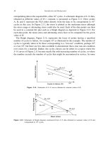
63 With reference to Fig. 4.6 we consider two cases: normal and shear strain.
Normal Strain: When Eq. 4.85 is applied to the differential element P
0
Q
0
which lies along the X
2
axis, the result will be the normal strain because since
d
X
1
dX
=
d
X
3
dX
=0and
d

X
2
dX
= 1. Therefore,
Eq. 4.85 becomes (with u
i
= x
i
− X
i
):
dx −dX
dX
= E
22
=
∂u
2
∂X
2
(4.86)
Victor Saouma Mechanics of Materials II
Draft
18 KINEMATIC
0
P
0
dX
2
X

X
X
2
Q
3
P
1
0
M
u
X
X
X
dX
1
2
3
dX
3
Normal
Shear
P
0
Q
0
2
1
x
x
x

M
Q
e
e
1
2
e
3
3
2
n
n
θ
3
Figure 4.6: Physical Interpretation of the Strain Tensor
Likewise for the other 2 directions. Hence the diagonal terms of the linear strain tensor represent
normal strains in the coordinate system.
Shear Strain: For the diagonal terms E
ij
we consider the two line elements originally located along
the X
2
and the X
3
axes before deformation. After deformation, the original right angle between
the lines becomes the angle θ. From Eq. 4.101 (du
i
=

∂u

i
∂X
j

P
0
dX
j
) a first order approximation
gives the unit vector at P in the direction of Q,andM as:
n
2
=
∂u
1
∂X
2
e
1
+ e
2
+
∂u
3
∂X
2
e
3
(4.87-a)
n

3
=
∂u
1
∂X
3
e
1
+
∂u
2
∂X
3
e
2
+ e
3
(4.87-b)
and from the definition of the dot product:
cos θ = n
2
·n
3
=
∂u
1
∂X
2
∂u
1

∂X
3
+
∂u
2
∂X
3
+
∂u
3
∂X
2
(4.88)
or neglecting the higher order term
cos θ =
∂u
2
∂X
3
+
∂u
3
∂X
2
=2E
23
(4.89)
64 Finally taking the change in right angle between the elements as γ
23
= π/2 − θ, and recalling

that for small strain theory γ
23
is very small it follows that
γ
23
≈ sin γ
23
=sin(π/2 −θ) = cos θ =2E
23
.
(4.90)
Victor Saouma Mechanics of Materials II
Draft
4.2 Strain Tensor 19
Therefore the off diagonal terms of the linear strain tensor represent one half of the angle change
between two line elements originally at right angles to one another. These components are called
the shear strains.
64 The Engineering shear strain is defined as one half the tensorial shear strain, and the resulting
tensor is written as
E
ij
=


ε
11
1
2
γ
12

1
2
γ
13
1
2
γ
12
ε
22
1
2
γ
23
1
2
γ
13
1
2
γ
23
ε
33


(4.91)
65 We note that a similar development paralleling the one just presented can be made for the linear
Eulerian strain tensor (where the straight lines and right angle will be in the deformed state).
4.2.5.2 Finite Strain; Stretch Ratio

66 The simplest and most useful measure of the extensional strain of an infinitesimal element is the
stretch or stretch ratio as
d
x
dX
which may be defined at point P
0
in the undeformed configuration or
at P in the deformed one (Refer to the original definition given by Eq, 4.1).
67 Hence, from Eq. 4.57-a, and Eq. 4.63 the squared stretch at P
0
for the line element along the unit
vector m =
d
X
dX
is given by
Λ
2
m
≡

dx
dX

2
P
0
= C
ij

dX
i
dX
dX
j
dX
or Λ
2
m
= m·C·m (4.92)
Thus for an element originally along X
2
, Fig. 4.6, m = e
2
and therefore dX
1
/dX =dX
3
/dX =0and
dX
2
/dX = 1, thus Eq. 4.92 (with Eq. ??) yields
Λ
2
e
2
= C
22
=1+2E
22

(4.93)
and similar results can be obtained for Λ
2
e
1
and Λ
2
e
3
.
68 Similarly from Eq. 4.53-b, the reciprocal of the squared stretch for the line element at P along the
unit vector n =
d
x
dx
is given by
1
λ
2
n
≡

dX
dx

2
P
= B
−1
ij

dx
i
dx
dx
j
dx
or
1
λ
2
n
= n·B
−1
·n (4.94)
Again for an element originally along X
2
, Fig. 4.6, we obtain
1
λ
2
e
2
=1−2E
∗
22
(4.95)
69 we note that in general Λ
e
2
= λ

e
2
since the element originally along the X
2
axis will not be along the
x
2
after deformation. Furthermore Eq. 4.92 and 4.94 show that in the matrices of rectangular cartesian
components the diagonal elements of both C and B
−1
must be positive, while the elements of E must
be greater than −
1
2
and those of E
∗
must be greater than +
1
2
.
70 The unit extension of the element is
dx −dX
dX
=
dx
dX
− 1=Λ
m
− 1 (4.96)
and for the element P

0
Q
0
along the X
2
axis, the unit extension is
dx −dX
dX
= E
(2)
=Λ
e
2
− 1=

1+2E
22
− 1 (4.97)
Victor Saouma Mechanics of Materials II
Draft
20 KINEMATIC
for small deformation theory E
22
<< 1, and
dx −dX
dX
= E
(2)
=(1+2E
22

)
1
2
− 1  1+
1
2
2E
22
− 1  E
22
(4.98)
which is identical to Eq. 4.86.
71 For the two differential line elements of Fig. 4.6, the change in angle γ
23
=
π
2
−θ is given in terms of
both Λ
e
2
and Λ
e
3
by
sin γ
23
=
2E
23

Λ
e
2
Λ
e
3
=
2E
23
√
1+2E
22
√
1+2E
33
(4.99)
Again, when deformations are small, this equation reduces to Eq. 4.90.
4.3 Strain Decomposition
72 In this section we first seek to express the relative displacement vector as the sum of the linear
(Lagrangian or Eulerian) strain tensor and the linear (Lagrangian or Eulerian) rotation tensor. This is
restricted to small strains.
73 For finite strains, the former additive decomposition is no longer valid, instead we shall consider the
strain tensor as a product of a rotation tensor and a stretch tensor.
4.3.1 †Linear Strain and Rotation Tensors
74 Strain components are quantitative measures of certain type of relative displacement between neigh-
boring parts of the material. A solid material will resist such relative displacement giving rise to internal
stresses.
75 Not all kinds of relative motion give rise to strain (and stresses). If a body moves as a rigid body,
the rotational part of its motion produces relative displacement. Thus the general problem is to express
the strain in terms of the displacements by separating off that part of the displacement distribution

which does not contribute to the strain.
4.3.1.1 Small Strains
76 From Fig. 4.7 the displacements of two neighboring particles are represented by the vectors u
P
0
and
u
Q
0
and the vector
du
i
= u
Q
0
i
− u
P
0
i
or du = u
Q
0
− u
P
0
(4.100)
is called the relative displacement vector of the particle originally at Q
0
with respect to the one

originally at P
0
.
4.3.1.1.1 Lagrangian Formulation
77 Neglecting higher order terms, and through a Taylor expansion
du
i
=

∂u
i
∂X
j

P
0
dX
j
or du =(u∇
X
)
P
0
dX (4.101)
78 We also define a unit relative displacement vector du
i
/dX where dX is the magnitude of the
differential distance dX
i
,ordX

i
= ξ
i
dX, then
du
i
dX
=
∂u
i
∂X
j
dX
j
dX
=
∂u
i
∂X
j
ξ
j
or
du
dX
= u∇
X
·ξ = J·ξ (4.102)
Victor Saouma Mechanics of Materials II
Draft

4.3 Strain Decomposition 21
0
Q
Q
0
0
p
Q
d X
d
u
d
x
u
u
P
0
P
Figure 4.7: Relative Displacement du of Q relative to P
79 The material displacement gradient
∂u
i
∂X
j
can be decomposed uniquely into a symmetric and an anti-
symetric part, we rewrite the previous equation as
du
i
=






1
2

∂u
i
∂X
j
+
∂u
j
∂X
i


 
E
ij
+
1
2

∂u
i
∂X
j
−

∂u
j
∂X
i


 
W
ij





dX
j
(4.103-a)
or
du =




1
2
(u∇
X
+ ∇
X
u)


 
E
+
1
2
(u∇
X
− ∇
X
u)

 
W




·dX (4.103-b)
or
E =





∂u
1
∂X
1

1
2

∂u
1
∂X
2
+
∂u
2
∂X
1

1
2

∂u
1
∂X
3
+
∂u
3
∂X
1

1
2

∂u

1
∂X
2
+
∂u
2
∂X
1

∂u
2
∂X
2
1
2

∂u
2
∂X
3
+
∂u
3
∂X
2

1
2

∂u

1
∂X
3
+
∂u
3
∂X
1

1
2

∂u
2
∂X
3
+
∂u
3
∂X
2

∂u
3
∂X
3






(4.104)
We thus introduce the linear lagrangian rotation tensor
W
ij
=
1
2

∂u
i
∂X
j
−
∂u
j
∂X
i

or W =
1
2
(u∇
X
− ∇
X
u)
(4.105)
in matrix form:
W =






0
1
2

∂u
1
∂X
2
−
∂u
2
∂X
1

1
2

∂u
1
∂X
3
−
∂u
3
∂X

1

−
1
2

∂u
1
∂X
2
−
∂u
2
∂X
1

0
1
2

∂u
2
∂X
3
−
∂u
3
∂X
2


−
1
2

∂u
1
∂X
3
−
∂u
3
∂X
1

−
1
2

∂u
2
∂X
3
−
∂u
3
∂X
2

0






(4.106)
80 In a displacement for which E
ij
is zero in the vicinity of a point P
0
, the relative displacement at that
point will be an infinitesimal rigid body rotation. It can be shown that this rotation is given by the
Victor Saouma Mechanics of Materials II
Draft
22 KINEMATIC
linear Lagrangian rotation vector
w
i
=
1
2

ijk
W
kj
or w =
1
2
∇
X
×u

(4.107)
or
w = −W
23
e
1
− W
31
e
2
− W
12
e
3
(4.108)
4.3.1.1.2 Eulerian Formulation
81 The derivation in an Eulerian formulation parallels the one for Lagrangian formulation. Hence,
du
i
=
∂u
i
∂x
j
dx
j
or du = K·dx (4.109)
82 The unit relative displacement vector will be
du
i

=
∂u
i
∂x
j
dx
j
dx
=
∂u
i
∂x
j
η
j
or
du
dx
= u∇
x
·η = K·β (4.110)
83 The decomposition of the Eulerian displacement gradient
∂u
i
∂x
j
results in
du
i
=







1
2

∂u
i
∂x
j
+
∂u
j
∂x
i


 
E
∗
ij
+
1
2

∂u
i

∂x
j
−
∂u
j
∂x
i


 
Ω
ij






dx
j
(4.111-a)
or
du =




1
2
(u∇

x
+ ∇
x
u)

 
E
∗
+
1
2
(u∇
x
− ∇
x
u)

 
Ω




·dx (4.111-b)
or
E =






∂u
1
∂x
1
1
2

∂u
1
∂x
2
+
∂u
2
∂x
1

1
2

∂u
1
∂x
3
+
∂u
3
∂x
1


1
2

∂u
1
∂x
2
+
∂u
2
∂x
1

∂u
2
∂x
2
1
2

∂u
2
∂x
3
+
∂u
3
∂x
2


1
2

∂u
1
∂x
3
+
∂u
3
∂x
1

1
2

∂u
2
∂x
3
+
∂u
3
∂x
2

∂u
3
∂x

3





(4.112)
84 We thus introduced the linear Eulerian rotation tensor
w
ij
=
1
2

∂u
i
∂x
j
−
∂u
j
∂x
i

or Ω =
1
2
(u∇
x
− ∇

x
u)
(4.113)
in matrix form:
W =





0
1
2

∂u
1
∂x
2
−
∂u
2
∂x
1

1
2

∂u
1
∂x

3
−
∂u
3
∂x
1

−
1
2

∂u
1
∂x
2
−
∂u
2
∂x
1

0
1
2

∂u
2
∂x
3
−

∂u
3
∂x
2

−
1
2

∂u
1
∂x
3
−
∂u
3
∂x
1

−
1
2

∂u
2
∂x
3
−
∂u
3

∂x
2

0





(4.114)
and the linear Eulerian rotation vector will be
ω
i
=
1
2

ijk
ω
kj
or ω =
1
2
∇
x
×u
(4.115)
Victor Saouma Mechanics of Materials II
Draft
4.3 Strain Decomposition 23

4.3.1.2 Examples
Example 4-8: Relative Displacement along a specified direction
A displacement field is specified by u = X
2
1
X
2
e
1
+(X
2
− X
2
3
)e
2
+ X
2
2
X
3
e
3
. Determine the relative
displacement vector du in the direction of the −X
2
axis at P (1, 2, −1). Determine the relative displace-
ments u
Q
i

− u
P
for Q
1
(1, 1, −1), Q
2
(1, 3/2, −1), Q
3
(1, 7/4, −1) and Q
4
(1, 15/8, −1) and compute their
directions with the direction of du.
Solution:
From Eq. 4.44, J = u∇
X
or
∂u
i
∂X
j
=


2X
1
X
2
X
2
1

0
01−2X
3
02X
2
X
3
X
2
2


(4.116)
thus from Eq. 4.101 du =(u∇
X
)
P
dX in the direction of −X
2
or
{du} =


410
012
0 −44






0
−1
0



=



−1
−1
4



(4.117)
By direct calculation from u we have
u
P
=2e
1
+ e
2
− 4e
3
(4.118-a)
u
Q

1
= e
1
− e
3
(4.118-b)
thus
u
Q
1
− u
P
= −e
1
− e
2
+3e
3
(4.119-a)
u
Q
2
− u
P
=
1
2
(−e
1
− e

2
+3.5e
3
) (4.119-b)
u
Q
3
− u
P
=
1
4
(−e
1
− e
2
+3.75e
3
) (4.119-c)
u
Q
4
− u
P
=
1
8
(−e
1
− e

2
+3.875e
3
) (4.119-d)
and it is clear that as Q
i
approaches P , the direction of the relative displacements of the two particles
approaches the limiting direction of du.
Example 4-9: Linear strain tensor, linear rotation tensor, rotation vector
Under the restriction of small deformation theory E = E
∗
, a displacement field is given by u =
(x
1
−x
3
)
2
e
1
+(x
2
+ x
3
)
2
e
2
−x
1

x
2
e
3
. Determine the linear strain tensor, the linear rotation tensor and
the rotation vector at point P (0, 2, −1).
Solution:
the matrix form of the displacement gradient is
[
∂u
i
∂x
j
]=


2(x
1
− x
3
)0−2(x
1
− x
3
)
02(x
2
+ x
3
)2(x

2
+ x
3
)
−x
2
−x
1
0


(4.120-a)

∂u
i
∂x
j

P
=


20−2
022
−20 0


(4.120-b)
Victor Saouma Mechanics of Materials II
Draft

24 KINEMATIC
Decomposing this matrix into symmetric and antisymmetric components give:
[E
ij
]+[w
ij
]=


20−2
021
−21 0


+


000
001
0 −10


(4.121)
and from Eq. Eq. 4.108
w = −W
23
e
1
− W
31

e
2
− W
12
e
3
= −1e
1
(4.122)
4.3.2 Finite Strain; Polar Decomposition
85 When the displacement gradients are finite, then we no longer can decompose
∂u
i
∂X
j
(Eq. 4.101) or
∂u
i
∂x
j
(Eq. 4.109) into a unique sum of symmetric and skew parts (pure strain and pure rotation).
86 Thus in this case, rather than having an additive decomposition, we will have a multiplicative
decomposition.
87 we call this a polar decomposition and it should decompose the deformation gradient in the product
of two tensors, one of which represents a rigid-body rotation, while the other is a symmetric positive-
definite tensor.
88 We apply this decomposition to the deformation gradient F:
F
ij
≡

∂x
i
∂X
j
= R
ik
U
kj
= V
ik
R
kj
or F = R·U = V·R
(4.123)
where R is the orthogonal rotation tensor,andU and V are positive symmetric tensors known as
the right stretch tensor and the left stretch tensor respectively.
89 The interpretation of the above equation is obtained by inserting the above equation into dx
i
=
∂x
i
∂X
j
dX
j
dx
i
= R
ik
U

kj
dX
j
= V
ik
R
kj
dX
j
or dx = R·U·dX = V·R·dX (4.124)
and we observe that in the first form the deformation consists of a sequential stretching (by U)and
rotation (R) to be followed by a rigid body displacement to x. In the second case, the orders are
reversed, we have first a rigid body translation to x, followed by a rotation (R) and finally a stretching
(by V).
90 To determine the stretch tensor from the deformation gradient
F
T
F =(RU)
T
(RU)=U
T
R
T
RU = U
T
U (4.125)
Recalling that R is an orthonormal matrix, and thus R
T
= R
−1

then we can compute the various
tensors from
U =
√
F
T
F (4.126)
R = FU
−1
(4.127)
V = FR
T
(4.128)
91 It can be shown that
U = C
1/2
and V = B
1/2
(4.129)
Example 4-10: Polar Decomposition I
Victor Saouma Mechanics of Materials II
Draft
4.3 Strain Decomposition 25
Given x
1
= X
1
, x
2
= −3X

3
, x
3
=2X
2
, find the deformation gradient F, the right stretch tensor U,
the rotation tensor R, and the left stretch tensor V.
Solution:
From Eq. 4.25
F =



∂x
1
∂X
1
∂x
1
∂X
2
∂x
1
∂X
3
∂x
2
∂X
1
∂x

2
∂X
2
∂x
2
∂X
3
∂x
3
∂X
1
∂x
3
∂X
2
∂x
3
∂X
3



=


10 0
00−3
02 0



(4.130)
From Eq. 4.126
U
2
= F
T
F =


100
002
0 −30




10 0
00−3
02 0


=


100
040
009


(4.131)

thus
U =


100
020
003


(4.132)
From Eq. 4.127
R = FU
−1
=


10 0
00−3
02 0




100
0
1
2
0
00
1

3


=


10 0
00−1
01 0


(4.133)
Finally, from Eq. 4.128
V = FR
T
=


10 0
00−3
02 0




100
001
0 −10



=


100
030
002


(4.134)
Example 4-11: Polar Decomposition II
For the following deformation: x
1
= λ
1
X
1
, x
2
= −λ
3
X
3
,andx
3
= λ
2
X
2
, find the rotation tensor.
Solution:

[F]=


λ
1
00
00−λ
3
0 λ
2
0


(4.135)
[U]
2
=[F]
T
[F] (4.136)
=


λ
1
00
00λ
2
0 −λ
3
0





λ
1
00
00−λ
3
0 λ
2
0


=


λ
2
1
00
0 λ
2
2
0
00λ
2
3



(4.137)
[U]=


λ
1
00
0 λ
2
0
00λ
3


(4.138)
[R]=[F][U]
−1
=


λ
1
00
00−λ
3
0 λ
2
0





1
λ
1
00
0
1
λ
2
0
00
1
λ
3


=


10 0
00−1
01 0


(4.139)
Thus we note that R corresponds to a 90
o
rotation about the e
1

axis.
Victor Saouma Mechanics of Materials II
Draft
4.3 Strain Decomposition 27
Polar Decomposition Using Mathematica
Given x
1
=X
1
+2X
2
, x
2
=X
2
, x
3
=X
3
, a) Obtain C, b) the principal values of C and the corresponding directions, c) the
matrix U and U
-1
with respect to the principal directions, d) Obtain the matrix U and U
-1
with respect to the e
i
bas
obtain the matrix R with respect to the e
i
basis.

Determine the F matrix
In[1]:= F = 881, 2, 0<, 80, 1, 0<, 80, 0, 1<<
Out[1]=
i
k
j
j
j
j
j
j
j
120
010
001
y
{
z
z
z
z
z
z
z
Solve for C
In[2]:= CST = Transpose@FD .F
Out[2]=
i
k
j

j
j
j
j
j
j
120
250
001
y
{
z
z
z
z
z
z
z
Determine Eigenvalues and Eigenvectors
In[3]:= N@Eigenvalues@CSTDD
Out[3]= 81., 0.171573, 5.82843<
In[4]:= 8v1, v2, v3< = N@Eigenvectors@CSTD,4D
Out[4]=
i
k
j
j
j
j
j

j
j
001.
-2.414 1. 0
0.4142 1. 0
y
{
z
z
z
z
z
z
z
In[5]:= << LinearAlgebra‘Orthogonalization‘
In[6]:= vnormalized = GramSchmidt@8v3, −v2, v1<D
Out[6]=
i
k
j
j
j
j
j
j
j
0.382683 0.92388 0
0.92388 -0.382683 0
001.
y

{
z
z
z
z
z
z
z
In[7]:= CSTeigen = Chop@N@vnormalized . CST . vnormalized, 4DD
Out[7]=
i
k
j
j
j
j
j
j
j
5.828 0 0
0 0.1716 0
001.
y
{
z
z
z
z
z
z

z
Determine U with respect to the principal directions
In[8]:= Ueigen = N@Sqrt@CSTeigenD,4D
Out[8]=
i
k
j
j
j
j
j
j
j
2.414 0 0
0 0.4142 0
001.
y
{
z
z
z
z
z
z
z
In[9]:= Ueigenminus1 = Inverse@UeigenD
Out[9]=
i
k
j

j
j
j
j
j
j
0.414214 0. 0.
0. 2.41421 0.
0. 0. 1.
y
{
z
z
z
z
z
z
z
2 m−
Determine U and U
-1
with respect to the e
i
basis
In[10]:= U_e = N@vnormalized . Ueigen . vnormalized, 3D
Out[10]=
i
k
j
j

j
j
j
j
j
0.707 0.707 0.
0.707 2.12 0.
0. 0. 1.
y
{
z
z
z
z
z
z
z
In[11]:= U_einverse = N@Inverse@%D,3D
Out[11]=
i
k
j
j
j
j
j
j
j
2.12 -0.707 0.
-0.707 0.707 0.

0. 0. 1.
y
{
z
z
z
z
z
z
z
Determine R with respect to the e
i
basis
In[12]:= R = N@F.%, 3D
Out[12]=
i
k
j
j
j
j
j
j
j
0.707 0.707 0.
-0.707 0.707 0.
0. 0. 1.
y
{
z

z
z
z
z
z
z
m−polar.nb
Victor Saouma Mechanics of Materials II
Draft
28 KINEMATIC
4.4 Summary and Discussion
92 From the above, we deduce the following observations:
1. If both the displacement gradients and the displacements themselves are small, then
∂u
i
∂X
j
≈
∂u
i
∂x
j
and
thus the Eulerian and the Lagrangian infinitesimal strain tensors may be taken as equal E
ij
= E
∗
ij
.
2. If the displacement gradients are small, but the displacements are large, we should use the Eulerian

infinitesimal representation.
3. If the displacements gradients are large, but the displacements are small, use the Lagrangian finite
strain representation.
4. If both the displacement gradients and the displacements are large, use the Eulerian finite strain
representation.
4.5 Compatibility Equation
93 If ε
ij
=
1
2
(u
i,j
+ u
j,i
) then we have six differential equations (in 3D the strain tensor has a total
of 9 terms, but due to symmetry, there are 6 independent ones) for determining (upon integration)
three unknowns displacements u
i
. Hence the system is overdetermined, and there must be some linear
relations between the strains.
94 It can be shown (through appropriate successive differentiation of the strain expression) that the
compatibility relation for strain reduces to:
∂
2
ε
ik
∂x
j
∂x

j
+
∂
2
ε
jj
∂x
i
∂x
k
−
∂
2
ε
jk
∂x
i
∂x
j
−
∂
2
ε
ij
∂x
j
∂x
k
=0. or ∇
x

×L×∇
x
=0
(4.140)
There are 81 equations in all, but only six are distinct
∂
2
ε
11
∂x
2
2
+
∂
2
ε
22
∂x
2
1
=2
∂
2
ε
12
∂x
1
∂x
2
(4.141-a)

∂
2
ε
22
∂x
2
3
+
∂
2
ε
33
∂x
2
2
=2
∂
2
ε
23
∂x
2
∂x
3
(4.141-b)
∂
2
ε
33
∂x

2
1
+
∂
2
ε
11
∂x
2
3
=2
∂
2
ε
31
∂x
3
∂x
1
(4.141-c)
∂
∂x
1

−
∂ε
23
∂x
1
+

∂ε
31
∂x
2
+
∂ε
12
∂x
3

=
∂
2
ε
11
∂x
2
∂x
3
(4.141-d)
∂
∂x
2

∂ε
23
∂x
1
−
∂ε

31
∂x
2
+
∂ε
12
∂x
3

=
∂
2
ε
22
∂x
3
∂x
1
(4.141-e)
∂
∂x
3

∂ε
23
∂x
1
+
∂ε
31

∂x
2
−
∂ε
12
∂x
3

=
∂
2
ε
33
∂x
1
∂x
2
(4.141-f)
In 2D, this results in (by setting i =2,j =1andl = 2):
∂
2
ε
11
∂x
2
2
+
∂
2
ε

22
∂x
2
1
=
∂
2
γ
12
∂x
1
∂x
2
(4.142)
Victor Saouma Mechanics of Materials II
Draft
4.5 Compatibility Equation 29
I , i
33
2
I , i
2
I , i
11
22
X , x
u
P
P
0

t=0
t=t
X
O
U
o
x
X , x
X , x
33
11
Material/Spatial
b=0
x
2
,
X
3
x
3
,
2
X
X
1
O
x
1
,
u

x
t=0
+d
X X
X
+d
d
d
x
t=t
X
u u
Q
0
Q
P
P
0
LAGRANGIAN EULERIAN
Material Spatial
Position Vector x = x(X,t) X = X(x,t)
GRADIENTS
Deformation F = x∇
X
≡
∂x
i
∂X
j
H = X∇

x
≡
∂X
i
∂x
j
H = F
−1
Displacement
∂u
i
∂X
j
=
∂x
i
∂X
j
− δ
ij
or
∂u
i
∂x
j
= δ
ij
−
∂X
i

∂x
j
or
J = u∇
X
= F − I K ≡ u∇
x
= I − H
TENSOR
dX
2
=dx·B
−1
·dx dx
2
=dX·C·dX
Cauchy Green
Deformation B
−1
ij
=
∂X
k
∂x
i
∂X
k
∂x
j
or C

ij
=
∂x
k
∂X
i
∂x
k
∂X
j
or
B
−1
= ∇
x
X·X∇
x
= H
c
·H C = ∇
X
x·x∇
X
= F
c
·F
C
−1
= B
−1

STRAINS
Lagrangian Eulerian/Almansi
dx
2
− dX
2
=dX·2E·dX dx
2
− dX
2
=dx·2E
∗
·dx
Finite Strain E
ij
=
1
2

∂x
k
∂X
i
∂x
k
∂X
j
− δ
ij


or
E
∗
ij
=
1
2

δ
ij
−
∂X
k
∂x
i
∂X
k
∂x
j

or
E =
1
2
(∇
X
x·x∇
X
  
F

c
·F
−I) E
∗
=
1
2
(I −∇
x
X·X∇
x
  
H
c
·H
)
E
ij
=
1
2

∂u
i
∂X
j
+
∂u
j
∂X

i
+
∂u
k
∂X
i
∂u
k
∂X
j

or
E
∗
ij
=
1
2

∂u
i
∂x
j
+
∂u
j
∂x
i
−
∂u

k
∂x
i
∂u
k
∂x
j

or
E =
1
2
(u∇
X
+ ∇
X
u + ∇
X
u·u∇
X
)

 
J+J
c
+J
c
·J
E
∗

=
1
2
(u∇
x
+ ∇
x
u −∇
x
u·u∇
x
)

 
K+K
c
−K
c
·K
Small E
ij
=
1
2

∂u
i
∂X
j
+

∂u
j
∂X
i

E
∗
ij
=
1
2

∂u
i
∂x
j
+
∂u
j
∂x
i

Deformation E =
1
2
(u∇
X
+ ∇
X
u)=

1
2
(J + J
c
) E
∗
=
1
2
(u∇
x
+ ∇
x
u)=
1
2
(K + K
c
)
ROTATION TENSORS
Small [
1
2

∂u
i
∂X
j
+
∂u

j
∂X
i

+
1
2

∂u
i
∂X
j
−
∂u
j
∂X
i

]dX
j

1
2

∂u
i
∂x
j
+
∂u

j
∂x
i

+
1
2

∂u
i
∂x
j
−
∂u
j
∂x
i

dx
j
deformation [
1
2
(u∇
X
+ ∇
X
u)

 

E
+
1
2
(u∇
X
− ∇
X
u)

 
W
]·dX [
1
2
(u∇
x
+ ∇
x
u)

 
E
∗
+
1
2
(u∇
x
− ∇

x
u)

 
Ω
]·dx
Finite Strain F = R·U = V·R
STRESS TENSORS
Piola-Kirchoff Cauchy
First T
0
= (det F)T

F
−1

T
Second
˜
T = (det F)

F
−1

T

F
−1

T

Table 4.1: Summary of Major Equations
Victor Saouma Mechanics of Materials II
Draft
30 KINEMATIC
(recall that 2ε
12
= γ
12
.)
95 When he compatibility equation is written in term of the stresses, it yields:
∂
2
σ
11
∂x
2
2
− ν
∂σ
22
2
∂x
2
2
+
∂
2
σ
22
∂x

2
1
− ν
∂
2
σ
11
∂x
2
1
=2(1+ν)
∂
2
σ
21
∂x
1
∂x
2
(4.143)
Example 4-13: Strain Compatibility
For the following strain field



−
X
2
X
2

1
+X
2
2
X
1
2(X
2
1
+X
2
2
)
0
X
1
2(X
2
1
+X
2
2
)
00
000



(4.144)
does there exist a single-valued continuous displacement field?

Solution:
∂E
11
∂X
2
= −
(X
2
1
+ X
2
2
) −X
2
(2X
2
)
(X
2
1
+ X
2
2
)
2
=
X
2
2
− X

2
1
(X
2
1
+ X
2
2
)
2
(4.145-a)
2
∂E
12
∂X
1
=
(X
2
1
+ X
2
2
) −X
1
(2X
1
)
(X
2

1
+ X
2
2
)
2
=
X
2
2
− X
2
1
(X
2
1
+ X
2
2
)
2
(4.145-b)
∂E
22
∂X
2
1
= 0 (4.145-c)
⇒
∂

2
E
11
∂X
2
2
+
∂
2
E
22
∂X
2
1
=2
∂
2
E
12
∂X
1
∂X
2
√
(4.145-d)
Actually, it can be easily verified that the unique displacement field is given by
u
1
= arctan
X

2
X
1
; u
2
=0; u
3
= 0 (4.146)
to which we could add the rigid body displacement field (if any).
4.6 Lagrangian Stresses; Piola Kirchoff Stress Tensors
96 In Sect. 2.2 the discussion of stress applied to the deformed configuration dA (using spatial coordiantes
x), that is the one where equilibrium must hold. The deformed configuration being the natural one in
which to characterize stress. Hence we had
df = tdA (4.147-a)
t = Tn (4.147-b)
(note the use of T instead of σ). Hence the Cauchy stress tensor was really defined in the Eulerian
space.
97 However, there are certain advantages in referring all quantities back to the undeformed configuration
(Lagrangian) of the body because often that configuration has geometric features and symmetries that
are lost through the deformation.
98 Hence, if we were to define the strain in material coordinates (in terms of X), we need also to express
the stress as a function of the material point X in material coordinates.
Victor Saouma Mechanics of Materials II
Draft
4.6 Lagrangian Stresses; Piola Kirchoff Stress Tensors 31
4.6.1 First
99 The first Piola-Kirchoff stress tensor T
0
is defined in the undeformed geometry in such a way that it
results in the same total force as the traction in the deformed configuration (where Cauchy’s stress

tensor was defined). Thus, we define
df ≡ t
0
dA
0
(4.148)
where t
0
is a pseudo-stress vector in that being based on the undeformed area, it does not describe
the actual intensity of the force, however it has the same direction as Cauchy’s stress vector t.
100 The first Piola-Kirchoff stress tensor (also known as Lagrangian Stress Tensor) is thus the linear
transformation T
0
such that
t
0
= T
0
n
0
(4.149)
and for which
df = t
0
dA
0
= tdA ⇒ t
0
=
dA

ddA
0
t (4.150)
using Eq. 4.147-b and 4.149 the preceding equation becomes
T
0
n
0
=
dA
dA
0
Tn = T
dA
dA
0
n (4.151)
and using Eq. 4.36 dAn =dA
0
(det F)

F
−1

T
n
0
we obtain
T
0

n
0
= T(det F)

F
−1

T
n
0
(4.152)
the above equation is true for all n
0
, therefore
T
0
= (det F)T

F
−1

T
(4.153)
T =
1
(det F)
T
0
F
T

or T
ij
=
1
(det F)
(T
0
)
im
F
jm
(4.154)
101 The first Piola-Kirchoff stress tensor is not symmetric in general, and is not energitically correct.
That is multiplying this stress tensor with the Green-Lagrange tensor will not be equal to the product
of the Cauchy stress tensor multiplied by the deformation strain tensor.
102 To determine the corresponding stress vector, we solve for T
0
first, then for dA
0
and n
0
from
dA
0
n
0
=
1
det F
F

T
n (assuming unit area dA), and finally t
0
= T
0
n
0
.
4.6.2 Second
103 The second Piola-Kirchoff stress tensor,
˜
T is formulated differently. Instead of the actual force df
on dA, it gives the force d
˜
f related to the force df in the same way that a material vector dX at X is
related by the deformation to the corresponding spatial vector dx at x. Thus, if we let
d
˜
f =
˜
tdA
0
(4.155-a)
and
df = Fd
˜
f (4.155-b)
where d
˜
f is the pseudo differential force which transforms, under the deformation gradient F,the

(actual) differential force df at the deformed position (note similarity with dx = FdX). Thus, the
pseudo vector t is in general in a differnt direction than that of the Cauchy stress vector t.
104 The second Piola-Kirchoff stress tensor is a linear transformation
˜
T such that
˜
t =
˜
Tn
0
(4.156)
Victor Saouma Mechanics of Materials II