Mechanics of Materials 2010 Part 6 ppsx

Draft
6.4 Conservation of Energy; First Principle of Thermodynamics 7
32 We thus have
dK
dt
+

V
D
ij
T
ij
dV =

V
(v
i
T
ji
)
,j
dV +

V
ρv
i
b
i
dV + Q (6.27)
33 We next convert the first integral on the right hand side to a surface integral by the divergence theorem
(


V
∇·TdV =

S
T.ndS) and since t
i
= T
ij
n
j
we obtain
dK
dt
+

V
D
ij
T
ij
dV =

S
v
i
t
i
dS +


V
ρv
i
b
i
dV + Q (6.28)
dK
dt
+
dU
dt
=
dW
dt
+ Q (6.29)
this equation relates the time rate of change of total mechanical energy of the continuum on the left side
to the rate of work done by the surface and body forces on the right hand side.
34 If both mechanical and non mechanical energies are to be considered, the first principle states that the
time rate of change of the kinetic plus the internal energy is equal to the sum of the rate of work plus all
other energies supplied to, or removed from the continuum per unit time (heat, chemical, electromagnetic,
etc.).
35 For a thermomechanical continuum, it is customary to express the time rate of change of internal
energy by the integral expression
dU
dt
=
d
dt

V

ρudV (6.30)
where u is the internal energy per unit mass or specific internal energy. We note that U appears
only as a differential in the first principle, hence if we really need to evaluate this quantity, we need to
have a reference value for which U will be null. The dimension of U is one of energy dim U = ML
2
T
−2
,
and the SI unit is the Joule, similarly dim u = L
2
T
−2
with the SI unit of Joule/Kg.
36 In terms of energy integrals, the first principle can be rewritten as
Rate of increase

 
d
dt

V
1
2
ρv
i
v
i
dV

 

dK
dt
=
˙
K
+
d
dt

V
ρudV

 
dU
dt
=
˙
U
=
Exchange

 

S
t
i
v
i
dS +
Source


 

V
ρv
i
b
i
dV

 
dW
dt
(P
ext
)
+
Source

 

V
ρrdV −
Exchange

 

S
q
i

n
i
dS

 
Q(P
cal
)
(6.31)
37 † If we apply Gauss theorem and convert the surface integral, collect terms and use the fact that dV
is arbitrary we obtain
ρ
du
dt
= T:D + ρr − ∇·q (6.32)
or (6.33)
ρ
du
dt
= T
ij
D
ij
+ ρr −
∂q
j
∂x
j
(6.34)
This equation expresses the rate of change of internal energy as the sum of the stress power plus

the heat added to the continuum.
38 In ideal elasticity, heat transfer is considered insignificant, and all of the input work is assumed
converted into internal energy in the form of recoverable stored elastic strain energy, which can be
recovered as work when the body is unloaded.
39 In general, however, the major part of the input work into a deforming material is not recoverably
stored, but dissipated by the deformation process causing an increase in the body’s temperature and
eventually being conducted away as heat.
Victor Saouma Mechanics of Materials II
Draft
8 FUNDAMENTAL LAWS of CONTINUUM MECHANICS
6.4.2 Local Form
40 Examining the third term in Eq. 6.31

S
t
i
v
i
dS =

S
v
i
T
ij
n
j
dS =

V

∂(v
i
T
ij
)
∂x
j
dV (6.35-a)
=

V
T
ij
∂v
i
∂x
j
dV +

V
v
i
∂T
ij
∂x
j
dV =

V
T:

˙
εdV +

V
v·(∇·T)dV (6.35-b)
41 We now evaluate P
ext
in Eq. 6.31
P
ext
=

S
t
i
v
i
dS +

V
ρv
i
b
i
dV (6.36-a)
=

V
v·(ρb + ∇·T)dV +


V
T:
˙
εdV (6.36-b)
Using Eq. 6.17 (T
ij,j
+ ρb
i
= ρ ˙v
i
), this reduces to
P
ext
=

V
v·(ρ
˙
v)dV

 
dK
+

V
T:
˙
εdV

 

P
int
(6.37)
(note that P
int
corresponds to the stress power).
42 Hence, we can rewrite Eq. 6.31 as
˙
U = P
int
+ P
cal
=

V
T:
˙
εdV +

V
(ρr − ∇·q)dV (6.38)
Introducing the specific internal energy u (taken per unit mass), we can express the internal energy of
the finite body as U =

V
ρudV , and rewrite the previous equation as

V
(ρ ˙u −T:
˙

ε − ρr + ∇·q)dV = 0 (6.39)
Since this equation must hold for any arbitrary partial volume V , we obtain the local form of the First
Law
ρ ˙u = T:
˙
ε + ρr − ∇·q
(6.40)
or the rate of increase of internal energy in an elementary material volume is equal to the sum of 1) the
power of stress T working on the strain rate
˙
ε, 2) the heat supplied by an internal source of intensity
r, and 3) the negative divergence of the heat flux which represents the net rate of heat entering the
elementary volume through its boundary.
6.5 Second Principle of Thermodynamics
6.5.1 Equation of State
43 The complete characterization of a thermodynamic system is said to describe the state of a system
(here a continuum). This description is specified, in general, by several thermodynamic and kinematic
state variables. A change in time of those state variables constitutes a thermodynamic process.
Usually state variables are not all independent, and functional relationships exist among them through
Victor Saouma Mechanics of Materials II
Draft
6.5 Second Principle of Thermodynamics 9
equations of state. Any state variable which may be expressed as a single valued function of a set of
other state variables is known as a state function.
44 The first principle of thermodynamics can be regarded as an expression of the interconvertibility of
heat and work, maintaining an energy balance. It places no restriction on the direction of the process.
In classical mechanics, kinetic and potential energy can be easily transformed from one to the other in
the absence of friction or other dissipative mechanism.
45 The first principle leaves unanswered the question of the extent to which conversion process is re-
versible or irreversible. If thermal processes are involved (friction) dissipative processes are irreversible

processes, and it will be up to the second principle of thermodynamics to put limits on the direction of
such processes.
6.5.2 Entropy
46 The basic criterion for irreversibility is given by the second principle of thermodynamics through
the statement on the limitation of entropy production. This law postulates the existence of two
distinct state functions: θ the absolute temperature and S the entropy with the following properties:
1. θ is a positive quantity.
2. Entropy is an extensive property, i.e. the total entropy in a system is the sum of the entropies of
its parts.
47 Thus we can write
ds =ds
(e)
+ds
(i)
(6.41)
where ds
(e)
is the increase due to interaction with the exterior, and ds
(i)
is the internal increase, and
ds
(e)
> 0 irreversible process (6.42-a)
ds
(i)
= 0 reversible process (6.42-b)
48 Entropy expresses a variation of energy associated with a variation in the temperature.
6.5.2.1 †Statistical Mechanics
49 In statistical mechanics, entropy is related to the probability of the occurrence of that state among
all the possible states that could occur. It is found that changes of states are more likely to occur in the

direction of greater disorder when a system is left to itself. Thus increased entropy means increased
disorder.
50 Hence Boltzman’s principle postulates that entropy of a state is proportional to the logarithm of its
probability, and for a gas this would give
S = kN[ln V +
3
2
lnθ]+C (6.43)
where S is the total entropy, V is volume, θ is absolute temperature, k is Boltzman’s constant, and C
is a constant and N is the number of molecules.
6.5.2.2 Classical Thermodynamics
51 In a reversible process (more about that later), the change in specific entropy s is given by
ds =

dq
θ

rev
(6.44)
Victor Saouma Mechanics of Materials II
Draft
10 FUNDAMENTAL LAWS of CONTINUUM MECHANICS
52 †If we consider an ideal gas governed by
pv = Rθ (6.45)
where R is the gas constant, and assuming that the specific energy u is only a function of temperature
θ, then the first principle takes the form
du =dq − pdv (6.46)
and for constant volume this gives
du =dq = c
v

dθ (6.47)
wher c
v
is the specific heat at constant volume. The assumption that u = u(θ) implies that c
v
is a
function of θ only and that
du = c
v
(θ)dθ (6.48)
53 †Hence we rewrite the first principle as
dq = c
v
(θ)dθ + Rθ
dv
v
(6.49)
or division by θ yields
s − s
0
=

p,v
p
0
,v
0
dq
θ
=


θ
θ
0
c
v
(θ)
dθ
θ
+ R ln
v
v
0
(6.50)
which gives the change in entropy for any reversible process in an ideal gas. In this case, entropy is a
state function which returns to its initial value whenever the temperature returns to its initial value that
is p and v return to their initial values.
54 The Clausius-Duhem inequality, an important relation associated with the second principle, will be
separately examined in Sect. 18.2.
6.6 Balance of Equations and Unknowns
55 In the preceding sections several equations and unknowns were introduced. Let us count them. for
both the coupled and uncoupled cases.
Coupled Uncoupled
dρ
dt
+ ρ
∂v
i
∂x
i

=0 Continuity Equation 1 1
∂T
ij
∂x
j
+ ρb
i
= ρ
dv
i
dt
Equation of motion 3 3
ρ
du
dt
= T
ij
D
ij
+ ρr −
∂q
j
∂x
j
Energy equation 1
Total number of equations 5 4
56 Assuming that the body forces b
i
and distributed heat sources r are prescribed, then we have the
following unknowns:

Coupled Uncoupled
Density ρ 1 1
Velocity (or displacement) v
i
(u
i
) 3 3
Stress components T
ij
6 6
Heat flux components q
i
3 -
Specific internal energy u 1 -
Entropy density s 1 -
Absolute temperature θ 1 -
Total number of unknowns 16 10
Victor Saouma Mechanics of Materials II
Draft
6.6 Balance of Equations and Unknowns 11
and in addition the Clausius-Duhem inequality
d
s
dt
≥
r
θ
−
1
ρ

div
q
θ
which governs entropy production must
hold.
57 We thus need an additional 16 −5 = 11 additional equations to make the system determinate. These
will be later on supplied by:
6 constitutive equations
3 temperature heat conduction
2 thermodynamic equations of state
11 Total number of additional equations
58 The next chapter will thus discuss constitutive relations, and a subsequent one will separately discuss
thermodynamic equations of state.
59 We note that for the uncoupled case
1. The energy equation is essentially the integral of the equation of motion.
2. The 6 missing equations will be entirely supplied by the constitutive equations.
3. The temperature field is regarded as known, or at most, the heat-conduction problem must be
solved separately and independently from the mechanical problem.
Victor Saouma Mechanics of Materials II
Draft
Chapter 7
CONSTITUTIVE EQUATIONS;
Part I Engineering Approach
ceiinosssttuu
Hooke, 1676
Ut tensio sic vis
Hooke, 1678
7.1 Experimental Observations
1 We shall discuss two experiments which will yield the elastic Young’s modulus, and then the bulk
modulus. In the former, the simplicity of the experiment is surrounded by the intriguing character of

Hooke, and in the later, the bulk modulus is mathematically related to the Green deformation tensor
C, the deformation gradient F and the Lagrangian strain tensor E.
7.1.1 Hooke’s Law
2 Hooke’s Law is determined on the basis of a very simple experiment in which a uniaxial force is applied
on a specimen which has one dimension much greater than the other two (such as a rod). The elongation
is measured, and then the stress is plotted in terms of the strain (elongation/length). The slope of the
line is called Young’s modulus.
3 Hooke anticipated some of the most important discoveries and inventions of his time but failed to carry
many of them through to completion. He formulated the theory of planetary motion as a problem in
mechanics, and grasped, but did not develop mathematically, the fundamental theory on which Newton
formulated the law of gravitation.
His most important contribution was published in 1678 in the paper De Potentia Restitutiva.It
contained results of his experiments with elastic bodies, and was the first paper in which the elastic
properties of material was discussed.
“Take a wire string of 20, or 30, or 40 ft long, and fasten the upper part thereof to a nail,
and to the other end fasten a Scale to receive the weights: Then with a pair of compasses take
the distance of the bottom of the scale from the ground or floor underneath, and set down the
said distance, then put inweights into the said scale and measure the several stretchings of
the said string, and set them down. Then compare the several stretchings of the said string,
and you will find that they will always bear the same proportions one to the other that the
weights do that made them”.
Draft
2 CONSTITUTIVE EQUATIONS; Part I Engineering Approach
This became Hooke’s Law
σ = Eε
(7.1)
4 Because he was concerned about patent rights to his invention, he did not publish his law when first
discovered it in 1660. Instead he published it in the form of an anagram “ceiinosssttuu” in 1676 and
the solution was given in 1678. Ut tensio sic vis (at the time the two symbols u and v were employed
interchangeably to denote either the vowel u or the consonant v), i.e. extension varies directly with force.

7.1.2 Bulk Modulus
5 If, instead of subjecting a material to a uniaxial state of stress, we now subject it to a hydrostatic
pressure p and measure the change in volume ∆V .
6 From the summary of Table 4.1 we know that:
V = (det F)V
0
(7.2-a)
det F =
√
det C =

det[I +2E] (7.2-b)
therefore,
V +∆V
V
=

det[I +2E] (7.3)
we can expand the determinant of the tensor det[I +2E]tofind
det[I +2E]=1+2I
E
+4II
E
+8III
E
(7.4)
but for small strains, I
E
 II
E

 III
E
since the first term is linear in E, the second is quadratic, and
the third is cubic. Therefore, we can approximate det[I+2E] ≈ 1+2I
E
, hence we define the volumetric
dilatation as
∆V
V
≡ e ≈ I
E
=trE
(7.5)
this quantity is readily measurable in an experiment.
7.2 Stress-Strain Relations in Generalized Elasticity
7.2.1 Anisotropic
7 From Eq. 18.31 and 18.32 we obtain the stress-strain relation for homogeneous anisotropic material
















T
11
T
22
T
33
T
12
T
23
T
31

















 
T
ij
=








c
1111
c
1112
c
1133
c
1112
c
1123
c
1131
c
2222
c
2233
c
2212

c
2223
c
2231
c
3333
c
3312
c
3323
c
3331
c
1212
c
1223
c
1231
SYM. c
2323
c
2331
c
3131










 
c
ijkm















E
11
E
22
E
33
2E
12
(γ

12
)
2E
23
(γ
23
)
2E
31
(γ
31
)
















 
E

km
(7.6)
which is Hooke’s law for small strain in linear elasticity.
8 †We also observe that for symmetric c
ij
we retrieve Clapeyron formula
W =
1
2
T
ij
E
ij
(7.7)
Victor Saouma Mechanics of Materials II
Draft
7.2 Stress-Strain Relations in Generalized Elasticity 3
9 In general the elastic moduli c
ij
relating the cartesian components of stress and strain depend on the
orientation of the coordinate system with respect to the body. If the form of elastic potential function
W and the values c
ij
are independent of the orientation, the material is said to be isotropic, if not it
is anisotropic.
10 c
ijkm
is a fourth order tensor resulting with 3
4
= 81 terms.

















c
1,1,1,1
c
1,1,1,2
c
1,1,1,3
c
1,1,2,1
c
1,1,2,2
c
1,1,2,3
c
1,1,3,1

c
1,1,3,2
c
1,1,3,3




c
1,2,1,1
c
1,2,1,2
c
1,2,1,3
c
1,2,2,1
c
1,2,2,2
c
1,2,2,3
c
1,2,3,1
c
1,2,3,2
c
1,2,3,3





c
1,3,1,1
c
1,3,1,2
c
1,3,1,3
c
1,3,2,1
c
1,3,2,2
c
1,3,2,3
c
1,3,3,1
c
1,3,3,2
c
1,3,3,3




c
2,1,1,1
c
2,1,1,2
c
2,1,1,3
c
2,1,2,1

c
2,1,2,2
c
2,1,2,3
c
2,1,3,1
c
2,1,3,2
c
2,1,3,3




c
2,2,1,1
c
2,2,1,2
c
2,2,1,3
c
2,2,2,1
c
2,2,2,2
c
2,2,2,3
c
2,2,3,1
c
2,2,3,2

c
2,2,3,3




c
2,3,1,1
c
2,3,1,2
c
2,3,1,3
c
2,3,2,1
c
2,3,2,2
c
2,3,2,3
c
2,3,3,1
c
2,3,3,2
c
2,3,3,3




c
3,1,1,1

c
3,1,1,2
c
3,1,1,3
c
3,1,2,1
c
3,1,2,2
c
3,1,2,3
c
3,1,3,1
c
3,1,3,2
c
3,1,3,3




c
3,2,1,1
c
3,2,1,2
c
3,2,1,3
c
3,2,2,1
c
3,2,2,2

c
3,2,2,3
c
3,2,3,1
c
3,2,3,2
c
3,2,3,3




c
3,3,1,1
c
3,3,1,2
c
3,3,1,3
c
3,3,2,1
c
3,3,2,2
c
3,3,2,3
c
3,3,3,1
c
3,3,3,2
c
3,3,3,3

















(7.8)
But the matrix must be symmetric thanks to Cauchy’s second law of motion (i.e symmetry of both the
stress and the strain), and thus for anisotropic material we will have a symmetric 6 by 6 matrix with
(6)(6+1)
2
= 21 independent coefficients.
11 †By means of coordinate transformation we can relate the material properties in one coordinate system
(old) x
i
,toanewonex
i
, thus from Eq. 1.39 (v
j
= a

p
j
v
p
) we can rewrite
W =
1
2
c
rstu
E
rs
E
tu
=
1
2
c
rstu
a
r
i
a
s
j
a
t
k
a
u

m
E
ij
E
km
=
1
2
c
ijkm
E
ij
E
km
(7.9)
thus we deduce
c
ijkm
= a
r
i
a
s
j
a
t
k
a
u
m

c
rstu
(7.10)
that is the fourth order tensor of material constants in old coordinates may be transformed into a new
coordinate system through an eighth-order tensor a
r
i
a
s
j
a
t
k
a
u
m
7.2.2 †Monotropic Material
12 A plane of elastic symmetry exists at a point where the elastic constants have the same values
for every pair of coordinate systems which are the reflected images of one another with respect to the
plane. The axes of such coordinate systems are referred to as “equivalent elastic directions”.
13 If we assume x
1
= x
1
, x
2
= x
2
and x
3

= −x
3
, then the transformation x
i
= a
j
i
x
j
is defined through
a
j
i
=


10 0
01 0
00−1


(7.11)
where the negative sign reflects the symmetry of the mirror image with respect to the x
3
plane.
14 We next substitute in Eq.7.10, and as an example we consider c
1123
= a
r
1

a
s
1
a
t
2
a
u
3
c
rstu
= a
1
1
a
1
1
a
2
2
a
3
3
c
1123
=
(1)(1)(1)(−1)c
1123
= −c
1123

, obviously, this is not possible, and the only way the relation can remanin
valid is if c
1123
= 0. We note that all terms in c
ijkl
with the index 3 occurring an odd number of times
will be equal to zero. Upon substitution, we obtain
c
ijkm
=








c
1111
c
1122
c
1133
c
1112
00
c
2222
c

2233
c
2212
00
c
3333
c
3312
00
c
1212
00
SYM. c
2323
c
2331
c
3131








(7.12)
we now have 13 nonzero coefficients.
Victor Saouma Mechanics of Materials II
Draft

4 CONSTITUTIVE EQUATIONS; Part I Engineering Approach
7.2.3 † Orthotropic Material
15 If the material possesses three mutually perpendicular planes of elastic symmetry, (that is symmetric
with respect to two planes x
2
and x
3
), then the transformation x
i
= a
j
i
x
j
is defined through
a
j
i
=


10 0
0 −10
00−1


(7.13)
where the negative sign reflects the symmetry of the mirror image with respect to the x
3
plane. Upon

substitution in Eq.7.10 we now would have
c
ijkm
=








c
1111
c
1122
c
1133
000
c
2222
c
2233
000
c
3333
000
c
1212
00

SYM. c
2323
0
c
3131








(7.14)
We note that in here all terms of c
ijkl
with the indices 3 and 2 occuring an odd number of times are
again set to zero.
16 Wood is usually considered an orthotropic material and will have 9 nonzero coefficients.
7.2.4 †Transversely Isotropic Material
17 A material is transversely isotropic if there is a preferential direction normal to all but one of the
three axes. If this axis is x
3
, then rotation about it will require that
a
j
i
=



cos θ sin θ 0
−sin θ cos θ 0
001


(7.15)
substituting Eq. 7.10 into Eq. 7.18, using the above transformation matrix, we obtain
c
1111
= (cos
4
θ)c
1111
+ (cos
2
θ sin
2
θ)(2c
1122
+4c
1212
) + (sin
4
θ)c
2222
(7.16-a)
c
1122
= (cos
2

θ sin
2
θ)c
1111
+ (cos
4
θ)c
1122
− 4(cos
2
θ sin
2
θ)c
1212
+(sin
4
θ)c
2211
(7.16-b)
+(sin
2
θ cos
2
θ)c
2222
(7.16-c)
c
1133
= (cos
2

θ)c
1133
+(sin
2
θ)c
2233
(7.16-d)
c
2222
=(sin
4
θ)c
1111
+ (cos
2
θ sin
2
θ)(2c
1122
+4c
1212
) + (cos
4
θ)c
2222
(7.16-e)
c
1212
= (cos
2

θ sin
2
θ)c
1111
− 2(cos
2
θ sin
2
θ)c
1122
− 2(cos
2
θ sin
2
θ)c
1212
+ (cos
4
θ)c
1212
(7.16-f)
+(sin
2
θ cos
2
θ)c
2222
+sin
4
θc

1212
(7.16-g)
.
.
.
But in order to respect our initial assumption about symmetry, these results require that
c
1111
= c
2222
(7.17-a)
c
1133
= c
2233
(7.17-b)
c
2323
= c
3131
(7.17-c)
c
1212
=
1
2
(c
1111
− c
1122

) (7.17-d)
Victor Saouma Mechanics of Materials II
Draft
7.2 Stress-Strain Relations in Generalized Elasticity 5
yielding
c
ijkm
=








c
1111
c
1122
c
1133
000
c
2222
c
2233
000
c
3333

000
1
2
(c
1111
− c
1122
)0 0
SYM. c
2323
0
c
3131








(7.18)
we now have 5 nonzero coefficients.
18 It should be noted that very few natural or man-made materials are truly orthotropic (certain crystals
as topaz are), but a number are transversely isotropic (laminates, shist, quartz, roller compacted concrete,
etc ).
7.2.5 Isotropic Material
19 An isotropic material is symmetric with respect to every plane and every axis, that is the elastic
properties are identical in all directions.
20 To mathematically characterize an isotropic material, we require coordinate transformation with

rotation about x
2
and x
1
axes in addition to all previous coordinate transformations. This process will
enforce symmetry about all planes and all axes.
21 The rotation about the x
2
axis is obtained through
a
j
i
=


cos θ 0 −sin θ
01 0
sin θ 0cosθ


(7.19)
we follow a similar procedure to the case of transversely isotropic material to obtain
c
1111
= c
3333
(7.20-a)
c
3131
=

1
2
(c
1111
− c
1133
) (7.20-b)
22 next we perform a rotation about the x
1
axis
a
j
i
=


10 0
0cosθ sin θ
0 −sin θ cos θ


(7.21)
it follows that
c
1122
= c
1133
(7.22-a)
c
3131

=
1
2
(c
3333
− c
1133
) (7.22-b)
c
2323
=
1
2
(c
2222
− c
2233
) (7.22-c)
which will finally give
c
ijkm
=









c
1111
c
1122
c
1133
000
c
2222
c
2233
000
c
3333
000
a 00
SYM. b 0
c








(7.23)
Victor Saouma Mechanics of Materials II
Draft
6 CONSTITUTIVE EQUATIONS; Part I Engineering Approach

with a =
1
2
(c
1111
− c
1122
), b =
1
2
(c
2222
− c
2233
), and c =
1
2
(c
3333
− c
1133
).
23 If we denote c
1122
= c
1133
= c
2233
= λ and c
1212

= c
2323
= c
3131
= µ then from the previous relations
we determine that c
1111
= c
2222
= c
3333
= λ +2µ,or
c
ijkm
=








λ +2µλ λ000
λ +2µλ000
λ +2µ 000
µ 00
SYM. µ 0
µ









(7.24)
= λδ
ij
δ
km
+ µ(δ
ik
δ
jm
+ δ
im
δ
kj
) (7.25)
and we are thus left with only two independent non zero coefficients λ and µ which are called Lame’s
constants.
24 Substituting the last equation into Eq. 7.6,
T
ij
=[λδ
ij
δ
km

+ µ(δ
ik
δ
jm
+ δ
im
δ
kj
)]E
km
(7.26)
Or in terms of λ and µ, Hooke’s Law for an isotropic body is written as
T
ij
= λδ
ij
E
kk
+2µE
ij
or T = λI
E
+2µE (7.27)
E
ij
=
1
2µ

T

ij
−
λ
3λ +2µ
δ
ij
T
kk

or E =
−λ
2µ(3λ +2µ)
I
T
+
1
2µ
T (7.28)
25 It should be emphasized that Eq. 7.24 is written in terms of the Engineering strains (Eq. 7.6) that
is γ
ij
=2E
ij
for i = j. On the other hand the preceding equations are written in terms of the tensorial
strains E
ij
7.2.5.1 Engineering Constants
26 The stress-strain relations were expressed in terms of Lame’s parameters which can not be readily
measured experimentally. As such, in the following sections we will reformulate those relations in terms
of “engineering constants” (Young’s and the bulk’s modulus). This will be done for both the isotropic

and transversely isotropic cases.
7.2.5.1.1 Isotropic Case
7.2.5.1.1.1 Young’s Modulus
27 In order to avoid certain confusion between the strain E and the elastic constant E, we adopt the
usual engineering notation T
ij
→ σ
ij
and E
ij
→ ε
ij
28 If we consider a simple uniaxial state of stress in the x
1
direction (σ
11
= σ, σ
22
= σ
33
= 0), then from
Eq. 7.28
ε
11
=
λ + µ
µ(3λ +2µ)
σ (7.29-a)
ε
22

= ε
33
=
−λ
2µ(3λ +2µ)
σ (7.29-b)
0=ε
12
= ε
23
= ε
13
(7.29-c)
Victor Saouma Mechanics of Materials II
Draft
7.2 Stress-Strain Relations in Generalized Elasticity 7
29 Yet we have the elementary relations in terms engineering constants E Young’s modulus and ν
Poisson’s ratio
ε
11
=
σ
E
(7.30-a)
ν = −
ε
22
ε
11
= −

ε
33
ε
11
(7.30-b)
then it follows that
1
E
=
λ + µ
µ(3λ +2µ)
; ν =
λ
2(λ + µ)
(7.31)
λ =
νE
(1 + ν)(1 − 2ν)
; µ = G =
E
2(1 + ν)
(7.32)
30 Similarly in the case of pure shear in the x
1
x
3
and x
2
x
3

planes, we have
σ
21
= σ
12
= τ all other σ
ij
= 0 (7.33-a)
2ε
12
=
τ
G
(7.33-b)
and the µ is equal to the shear modulus G.
31 Hooke’s law for isotropic material in terms of engineering constants becomes
σ
ij
=
E
1+ν

ε
ij
+
ν
1 − 2ν
δ
ij
ε

kk

or σ =
E
1+ν

ε +
ν
1 − 2ν
I
ε

(7.34)
ε
ij
=
1+ν
E
σ
ij
−
ν
E
δ
ij
σ
kk
or ε =
1+ν
E

σ −
ν
E
I
σ
(7.35)
32 When the strain equation is expanded in 3D cartesian coordinates it would yield:















ε
xx
ε
yy
ε
zz
γ
xy

(2ε
xy
)
γ
yz
(2ε
yz
)
γ
zx
(2ε
zx
)















=
1

E








1 −ν −ν 000
−ν 1 −ν 000
−ν −ν 10 0 0
0001+ν 00
000 01+ν 0
000 0 01+ν
























σ
xx
σ
yy
σ
zz
τ
xy
τ
yz
τ
zx
















(7.36)
33 If we invert this equation, we obtain















σ
xx
σ
yy
σ
zz
τ
xy

τ
yz
τ
zx















=








E
(1+ν)(1−2ν)



1 − νν ν
ν 1 −νν
νν1 − ν


0
0 G


100
010
001


























ε
xx
ε
yy
ε
zz
γ
xy
(2ε
xy
)
γ
yz
(2ε
yz
)
γ
zx
(2ε
zx
)
















(7.37)
7.2.5.1.1.2 Bulk’s Modulus; Volumetric and Deviatoric Strains
34 We can express the trace of the stress I
σ
in terms of the volumetric strain I
ε
From Eq. 7.27
σ
ii
= λδ
ii
ε
kk
+2µε
ii

=(3λ +2µ)ε
ii
≡ 3Kε
ii
(7.38)
Victor Saouma Mechanics of Materials II
Draft
8 CONSTITUTIVE EQUATIONS; Part I Engineering Approach
or
K = λ +
2
3
µ
(7.39)
35 We can provide a complement to the volumetric part of the constitutive equations by substracting
the trace of the stress from the stress tensor, hence we define the deviatoric stress and strains as as
σ

≡ σ −
1
3
(tr σ)I (7.40)
ε

≡ ε −
1
3
(tr ε)I (7.41)
and the corresponding constitutive relation will be
σ = KeI +2µε


(7.42)
ε =
p
3K
I +
1
2µ
σ

(7.43)
where p ≡
1
3
tr (σ) is the pressure, and σ

= σ −pI is the stress deviator.
7.2.5.1.1.3 †Restriction Imposed on the Isotropic Elastic Moduli
36 We can rewrite Eq. 18.29 as
dW = T
ij
dE
ij
(7.44)
but since dW is a scalar invariant (energy), it can be expressed in terms of volumetric (hydrostatic) and
deviatoric components as
dW = −pde + σ

ij
dE


ij
(7.45)
substituting p = −Ke and σ

ij
=2GE

ij
, and integrating, we obtain the following expression for the
isotropic strain energy
W =
1
2
Ke
2
+ GE

ij
E

ij
(7.46)
and since positive work is required to cause any deformation W>0thus
λ +
2
3
G ≡ K>0 (7.47-a)
G>0 (7.47-b)
ruling out K = G = 0, we are left with

E>0; −1 <ν<
1
2
(7.48)
37 The isotropic strain energy function can be alternatively expressed as
W =
1
2
λe
2
+ GE
ij
E
ij
(7.49)
38 From Table 7.1, we observe that ν =
1
2
implies G =
E
3
,and
1
K
= 0 or elastic incompressibility.
39 The elastic properties of selected materials is shown in Table 7.2.
Victor Saouma Mechanics of Materials II
Draft
7.2 Stress-Strain Relations in Generalized Elasticity 9
λ, µ E, ν µ, ν E, µ K, ν

λ λ
νE
(1+ν)(1−2ν)
2µν
1−2ν
µ(E−2µ)
3µ−E
3Kν
1+ν
µ µ
E
2(1+ν)
µµ
3K(1−2ν)
2(1+ν)
K λ +
2
3
µ
E
3(1−2ν)
2µ(1+ν)
3(1−2ν)
µE
3(3µ−E)
K
E
µ(3λ+2µ)
λ+µ
E 2µ(1 + ν) E 3K(1 − 2ν)

ν
λ
2(λ+µ)
νν
E
2µ
− 1 ν
Table 7.1: Conversion of Constants for an Isotropic Elastic Material
Material E (MPa) ν
A316 Stainless Steel 196,000 0.3
A5 Aluminum 68,000 0.33
Bronze 61,000 0.34
Plexiglass 2,900 0.4
Rubber 2 →0.5
Concrete 60,000 0.2
Granite 60,000 0.27
Table 7.2: Elastic Properties of Selected Materials at 20
0c
7.2.5.1.2 †Transversly Isotropic Case
40 For transversely isotropic, we can express the stress-strain relation in tems of
ε
xx
= a
11
σ
xx
+ a
12
σ
yy

+ a
13
σ
zz
ε
yy
= a
12
σ
xx
+ a
11
σ
yy
+ a
13
σ
zz
ε
zz
= a
13
(σ
xx
+ σ
yy
)+a
33
σ
zz

γ
xy
=2(a
11
− a
12
)τ
xy
γ
yz
= a
44
τ
xy
γ
xz
= a
44
τ
xz
(7.50)
and
a
11
=
1
E
; a
12
= −

ν
E
; a
13
= −
ν

E

; a
33
= −
1
E

; a
44
= −
1
µ

(7.51)
where E is the Young’s modulus in the plane of isotropy and E

the one in the plane normal to it. ν
corresponds to the transverse contraction in the plane of isotropy when tension is applied in the plane;
ν

corresponding to the transverse contraction in the plane of isotropy when tension is applied normal
to the plane; µ


corresponding to the shear moduli for the plane of isotropy and any plane normal to it,
and µ is shear moduli for the plane of isotropy.
7.2.5.2 Special 2D Cases
41 Often times one can make simplifying assumptions to reduce a 3D problem into a 2D one.
7.2.5.2.1 Plane Strain
42 For problems involving a long body in the z direction with no variation in load or geometry, then
Victor Saouma Mechanics of Materials II
Draft
10 CONSTITUTIVE EQUATIONS; Part I Engineering Approach
ε
zz
= γ
yz
= γ
xz
= τ
xz
= τ
yz
= 0. Thus, replacing into Eq. 7.37 we obtain







σ
xx

σ
yy
σ
zz
τ
xy







=
E
(1 + ν)(1 − 2ν)




(1 − ν) ν 0
ν (1 − ν)0
νν0
00
1−2ν
2








ε
xx
ε
yy
γ
xy



(7.52)
7.2.5.2.2 Axisymmetry
43 In solids of revolution, we can use a polar coordinate sytem and
ε
rr
=
∂u
∂r
(7.53-a)
ε
θθ
=
u
r
(7.53-b)
ε
zz
=

∂w
∂z
(7.53-c)
ε
rz
=
∂u
∂z
+
∂w
∂r
(7.53-d)
44 The constitutive relation is again analogous to 3D/plane strain







σ
rr
σ
zz
σ
θθ
τ
rz








=
E
(1 + ν)(1 − 2ν)






1 − νν ν 0
ν 1 −νν 0
νν1 − ν 0
νν1 − ν 0
000
1−2ν
2














ε
rr
ε
zz
ε
θθ
γ
rz







(7.54)
7.2.5.2.3 Plane Stress
45 If the longitudinal dimension in z direction is much smaller than in the x and y directions, then
τ
yz
= τ
xz
= σ
zz
= γ
xz

= γ
yz
= 0 throughout the thickness. Again, substituting into Eq. 7.37 we
obtain:



σ
xx
σ
yy
τ
xy



=
1
1 − ν
2


1 ν 0
ν 10
00
1−ν
2






ε
xx
ε
yy
γ
xy



(7.55-a)
ε
zz
= −
1
1 − ν
ν(ε
xx
+ ε
yy
) (7.55-b)
7.3 †Linear Thermoelasticity
46 If thermal effects are accounted for, the components of the linear strain tensor E
ij
may be considered
as the sum of
E
ij
= E

(T )
ij
+ E
(Θ)
ij
(7.56)
where E
(T )
ij
is the contribution from the stress field, and E
(Θ)
ij
the contribution from the temperature
field.
47 When a body is subjected to a temperature change Θ − Θ
0
with respect to the reference state
temperature, the strain componenet of an elementary volume of an unconstrained isotropic body are
given by
E
(Θ)
ij
= α(Θ − Θ
0
)δ
ij
(7.57)
Victor Saouma Mechanics of Materials II
Draft
7.4 Fourrier Law 11

where α is the linear coefficient of thermal expansion.
48 Inserting the preceding two equation into Hooke’s law (Eq. 7.28) yields
E
ij
=
1
2µ

T
ij
−
λ
3λ +2µ
δ
ij
T
kk

+ α(Θ − Θ
0
)δ
ij
(7.58)
which is known as Duhamel-Neumann relations.
49 If we invert this equation, we obtain the thermoelastic constitutive equation:
T
ij
= λδ
ij
E

kk
+2µE
ij
− (3λ +2µ)αδ
ij
(Θ − Θ
0
)
(7.59)
50 Alternatively, if we were to consider the derivation of the Green-elastic hyperelastic equations, (Sect.
18.5.1), we required the constants c
1
to c
6
in Eq. 18.31 to be zero in order that the stress vanish in the
unstrained state. If we accounted for the temperature change Θ −Θ
0
with respect to the reference state
temperature, we would have c
k
= −β
k
(Θ − Θ
0
)fork = 1 to 6 and would have to add like terms to Eq.
18.31, leading to
T
ij
= −β
ij

(Θ − Θ
0
)+c
ijrs
E
rs
(7.60)
for linear theory, we suppose that β
ij
is independent from the strain and c
ijrs
independent of temperature
change with respect to the natural state. Finally, for isotropic cases we obtain
T
ij
= λE
kk
δ
ij
+2µE
ij
− β
ij
(Θ − Θ
0
)δ
ij
(7.61)
which is identical to Eq. 7.59 with β =
Eα

1−2ν
. Hence
T
Θ
ij
=
Eα
1 − 2ν
(7.62)
51 In terms of deviatoric stresses and strains we have
T

ij
=2µE

ij
and E

ij
=
T

ij
2µ
(7.63)
and in terms of volumetric stress/strain:
p = −Ke + β(Θ − Θ
0
)ande =
p

K
+3α(Θ − Θ
0
)
(7.64)
7.4 Fourrier Law
52 Consider a solid through which there is a flow q of heat (or some other quantity such as mass, chemical,
etc )
53 The rate of transfer per unit area is q
54 The direction of flow is in the direction of maximum “potential” (temperature in this case, but could
be, piezometric head, or ion concentration) decreases (Fourrier, Darcy, Fick ).
q =



q
x
q
y
q
z



= −D






∂φ
∂x
∂φ
∂y
∂φ
∂z





= −D∇φ (7.65)
Victor Saouma Mechanics of Materials II
Draft
12 CONSTITUTIVE EQUATIONS; Part I Engineering Approach
D is a three by three (symmetric) constitutive/conductivity matrix
The conductivity can be either
Isotropic
D = k


100
010
001


(7.66)
Anisotropic
D =



k
xx
k
xy
k
xz
k
yx
k
yy
k
yz
k
zx
k
zy
k
zz


(7.67)
Orthotropic
D =


k
xx
00
0 k

yy
0
00k
zz


(7.68)
Note that for flow through porous media, Darcy’s equation is only valid for laminar flow.
7.5 Updated Balance of Equations and Unknowns
55 In light of the new equations introduced in this chapter, it would be appropriate to revisit our balance
of equations and unknowns.
Coupled Uncoupled
dρ
dt
+ ρ
∂v
i
∂x
i
=0 Continuity Equation 1 1
∂T
ij
∂x
j
+ ρb
i
= ρ
dv
i
dt

Equation of motion 3 3
ρ
du
dt
= T
ij
D
ij
+ ρr −
∂q
j
∂x
j
Energy equation 1
T = λI
E
+2µE Hooke’s Law 6 6
q = −D∇φ Heat Equation (Fourrier) 3
Θ=Θ(s,ν); τ
j
= τ
j
(s, ν) Equations of state 2
Total number of equations 16 10
and we repeat our list of unknowns
Coupled Uncoupled
Density ρ 1 1
Velocity (or displacement) v
i
(u

i
) 3 3
Stress components T
ij
6 6
Heat flux components q
i
3 -
Specific internal energy u 1 -
Entropy density s 1 -
Absolute temperature Θ 1 -
Total number of unknowns 16 10
and in addition the Clausius-Duhem inequality
ds
dt
≥
r
Θ
−
1
ρ
div
q
Θ
which governs entropy production
must hold.
56 Hence we now have as many equations as unknowns and are (almost) ready to pose and solve problems
in continuum mechanics.
Victor Saouma Mechanics of Materials II
Draft

Part II
ELASTICITY/SOLID
MECHANICS
Draft
Chapter 8
BOUNDARY VALUE PROBLEMS
in ELASTICITY
8.1 Preliminary Considerations
1 All problems in elasticity require three basic components:
3 Equations of Motion (Equilibrium): i.e. Equations relating the applied tractions and body forces
to the stresses (3)
∂T
ij
∂X
j
+ ρb
i
= ρ
∂
2
u
i
∂t
2
(8.1)
6 Stress-Strain relations: (Hooke’s Law)
T = λI
E
+2µE (8.2)
6 Geometric (kinematic) equations: i.e. Equations of geometry of deformation relating displace-

ment to strain (6)
E
∗
=
1
2
(u∇
x
+ ∇
x
u) (8.3)
2 Those 15 equations are written in terms of 15 unknowns: 3 displacement u
i
, 6 stress components T
ij
,
and 6 strain components E
ij
.
3 In addition to these equations which describe what is happening inside the body, we must describe
what is happening on the surface or boundary of the body, just like for the solution of a differential
equation. These extra conditions are called boundary conditions.
8.2 Boundary Conditions
4 In describing the boundary conditions (B.C.), we must note that:
1. Either we know the displacement but not the traction, or we know the traction and not the
corresponding displacement. We can never know both a priori.
2. Not all boundary conditions specifications are acceptable. For example we can not apply tractions
to the entire surface of the body. Unless those tractions are specially prescribed, they may not
necessarily satisfy equilibrium.
Draft

2 BOUNDARY VALUE PROBLEMS in ELASTICITY
5 Properly specified boundary conditions result in well-posed boundary value problems, while improp-
erly specified boundary conditions will result in ill-posed boundary value problem. Only the former
can be solved.
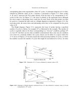
6 Thus we have two types of boundary conditions in terms of known quantitites, Fig. 8.1:
Ω
Γ
Τ
u
t
Figure 8.1: Boundary Conditions in Elasticity Problems
Displacement boundary conditions along Γ
u
with the three components of u
i
prescribed on the
boundary. The displacement is decomposed into its cartesian (or curvilinear) components, i.e.
u
x
,u
y
Traction boundary conditions along Γ
t
with the three traction components t
i
= n
j
T
ij
prescribed

at a boundary where the unit normal is n. The traction is decomposed into its normal and shear(s)
components, i.e t
n
,t
s
.
Mixed boundary conditions where displacement boundary conditions are prescribed on a part of
the bounding surface, while traction boundary conditions are prescribed on the remainder.
We note that at some points, traction may be specified in one direction, and displacement at another.
Displacement and tractions can never be specified at the same point in the same direction.
7 Various terms have been associated with those boundary conditions in the litterature, those are su-
umarized in Table 8.1.
u,Γ
u
t,Γ
t
Dirichlet Neuman
Field Variable Derivative(s) of Field Variable
Essential Non-essential
Forced Natural
Geometric Static
Table 8.1: Boundary Conditions in Elasticity
8 Often time we take advantage of symmetry not only to simplify the problem, but also to properly
define the appropriate boundary conditions, Fig. 8.2.
Victor Saouma Mechanics of Materials II