Mobile Robots Perception & Navigation Part 1 ppsx
Bạn đang xem bản rút gọn của tài liệu. Xem và tải ngay bản đầy đủ của tài liệu tại đây (769.24 KB, 40 trang )
Mobile Robots
Perception & Navigation
Mobile Robots
Perception & Navigation
Edited by
Sascha Kolski
pro literatur Verlag
Published by the Advanced Robotic Systems International and pro literatur Verlag
plV pro literatur Verlag Robert Mayer-Scholz
Mammendorf
Germany
Abstracting and non-profit use of the material is permitted with credit to the source. Statements and
opinions expressed in the chapters are these of the individual contributors and not necessarily those of
the editors or publisher. No responsibility is accepted for the accuracy of information contained in the
published articles. Publisher assumes no responsibility liability for any damage or injury to persons or
property arising out of the use of any materials, instructions, methods or ideas contained inside. After
this work has been published by the Advanced Robotic Systems International, authors have the right to
republish it, in whole or part, in any publication of which they are an author or editor, and the make
other personal use of the work.
© 2007 Advanced Robotic Systems International
www.ars-journal.com
Additional copies can be obtained from:
First published March 2007
Printed in Croatia
A catalog record for this book is available from the German Library.
Mobile Robots, Perception & Navigation, Edited by Sascha Kolski
p. cm.
ISBN 3-86611-283-1
1. Mobile Robotics. 2. Perception. 3. Sascha Kolski
V
Preface
Mobile Robotics is an active research area where researchers from all over the world find
new technologies to improve mobile robots intelligence and areas of application. Today ro-
bots navigate autonomously in office environments as well as outdoors. They show their
ability to beside mechanical and electronic barriers in building mobile platforms, perceiving
the environment and deciding on how to act in a given situation are crucial problems. In this
book we focused on these two areas of mobile robotics, Perception and Navigation.
Perception includes all means of collecting information about the robot itself and it’s envi-
ronment. To make robots move in their surrounding and interact with their environment in
a reasonable way, it is crucial to understand the actual situation the robot faces.
Robots use sensors to measure properties of the environment and interpret these measure-
ments to gather knowledge needed for save interaction. Sensors used in the work described
in the articles in this book include computer vision, range finders, sonars and tactile sensors
and the way those sensors can be used to allow the robot the perception of it’s environment
and enabling it to safely accomplishing it’s task. There is also a number of contributions that
show how measurements from different sensors can be combined to gather more reliable
and accurate information as a single sensor could provide, this is especially efficient when
sensors are complementary on their strengths and weaknesses.
As for many robot tasks mobility is an important issue, robots have to navigate their envi-
ronments in a safe and reasonable way. Navigation describes, in the field of mobile robotics,
techniques that allow a robot to use information it has gathered about the environment to
reach goals that are given a priory or derived from a higher level task description in an ef-
fective and efficient way.
The main question of navigation is how to get from where we are to where we want to be.
Researchers work on that question since the early days of mobile robotics and have devel-
oped many solutions to the problem considering different robot environments. Those in-
clude indoor environments, as well is in much larger scale outdoor environments and under
water navigation.
Beside the question of global navigation, how to get from A to B navigation in mobile robot-
ics has local aspects. Depending on the architecture of a mobile robot (differential drive, car
like, submarine, plain, etc.) the robot’s possible actions are constrained not only by the ro-
VI
bots’ environment but by its dynamics. Robot motion planning takes these dynamics into
account to choose feasible actions and thus ensure a safe motion.
This book gives a wide overview over different navigation techniques describing both navi-
gation techniques dealing with local and control aspects of navigation as well es those han-
dling global navigation aspects of a single robot and even for a group of robots.
As not only this book shows, mobile robotics is a living and exciting field of research com-
bining many different ideas and approaches to build mechatronical systems able to interact
with their environment.
Editor
Sascha Kolski
VII
Contents
Perception
1. Robot egomotion from the deformation of active contours
.
01
Guillem Alenya and Carme Torras
2. Visually Guided Robotics Using Conformal Geometric Computing 19
Eduardo Bayro-Corrochano, Luis Eduardo Falcon-Morales and
Julio Zamora-Esquivel
3. One approach To The Fusion Of Inertial Navigation
And Dynamic Vision 45
Stevica Graovac
4. Sonar Sensor Interpretation and Infrared Image
Fusion for Mobile Robotics 69
Mark Hinders, Wen Gao and William Fehlman
5. Obstacle Detection Based on Fusion Between
Stereovision and 2D Laser Scanner 91
Raphaël Labayrade, Dominique Gruyer, Cyril Royere,
Mathias Perrollaz and Didier Aubert
6. Optical Three-axis Tactile Sensor 111
Ohka, M.
7. Vision Based Tactile Sensor Using Transparent
Elastic Fingertip for Dexterous Handling 137
Goro Obinata, Dutta Ashish, Norinao Watanabe and Nobuhiko Moriyama
8. Accurate color classification and segmentation for mobile robots 149
Raziel Alvarez, Erik Millán, Alejandro Aceves-López and
Ricardo Swain-Oropeza
9. Intelligent Global Vision for Teams of Mobile Robots 165
Jacky Baltes and John Anderson
10. Contour Extraction and Compression-Selected Topics 187
Andrzej Dziech
VIII
Navigation
11. Comparative Analysis of Mobile Robot Localization Methods
Based On Proprioceptive and Exteroceptive Sensors
.
215
Gianluca Ippoliti, Leopoldo Jetto, Sauro Longhi and Andrea Monteriù
12. Composite Models for Mobile Robot Offline Path Planning
.
237
Ellips Masehian and M. R. Amin-Naseri
13. Global Navigation of Assistant Robots using Partially
Observable Markov Decision Processes
.
263
María Elena López, Rafael Barea, Luis Miguel Bergasa,
Manuel Ocaña and María Soledad Escudero
14. Robust Autonomous Navigation and World
Representation in Outdoor Environments 299
Favio Masson, Juan Nieto, José Guivant and Eduardo Nebot
15. Unified Dynamics-based Motion Planning Algorithm for
Autonomous Underwater Vehicle-Manipulator Systems (UVMS) 321
Tarun K. Podder and Nilanjan Sarkar
16. Optimal Velocity Planning of Wheeled Mobile Robots on
Specific Paths in Static and Dynamic Environments
.
357
María Prado
17. Autonomous Navigation of Indoor Mobile Robot
Using Global Ultrasonic System 383
Soo-Yeong Yi and Byoung-Wook Choi
18. Distance Feedback Travel Aid Haptic Display Design 395
Hideyasu Sumiya
19. Efficient Data Association Approach to Simultaneous
Localization and Map Building 413
Sen Zhang, Lihua Xie and Martin David Adams
20. A Generalized Robot Path Planning Approach Without
The Cspace Calculation 433
Yongji Wang, Matthew Cartmell, QingWang and Qiuming Tao
21. A pursuit-rendezvous approach for robotic tracking
.
461
Fethi Belkhouche and Boumediene Belkhouche
22. Sensor-based Global Planning for Mobile Manipulators
Navigation using Voronoi Diagram and Fast Marching 479
S. Garrido, D. Blanco, M.L. Munoz, L. Moreno and M. Abderrahim
IX
23. Effective method for autonomous Simultaneous Localization
and Map building in unknown indoor environments 497
Y.L. Ip, A.B. Rad, and Y.K. Wong
24. Motion planning and reconfiguration for systems of
multiple objects 523
Adrian Dumitrescu
25. Symbolic trajectory description in mobile robotics 543
Pradel Gilbert and Caleanu Catalin-Daniel
26. Robot Mapping and Navigation by Fusing Sensory Information
.
571
Maki K. Habib
27. Intelligent Control of AC Induction Motors 595
Hosein Marzi
28. Optimal Path Planning of Multiple Mobile Robots for
Sample Collection on a Planetary Surface
.
605
J.C. Cardema and P.K.C. Wang
29. Multi Robotic Conflict Resolution by Cooperative Velocity
and Direction Control 637
Satish Pedduri and K Madhava Krishna
30. Robot Collaboration For Simultaneous Map Building
and Localization
.
667
M. Oussalah and D. Wilson
X
1
Robot Egomotion from the Deformation of
Active Contours
Guillem ALENYA and Carme TORRAS
Institut de Robòtica i Informàtica Industrial (CSIC-UPC) Barcelona, Catalonia, Spain
1.Introduction
Traditional sources of information for image-based computer vision algorithms have been
points, lines, corners, and recently SIFT features (Lowe, 2004), which seem to represent at
present the state of the art in feature definition. Alternatively, the present work explores the
possibility of using tracked contours as informative features, especially in applications not
requiring high precision as it is the case of robot navigation.
In the past two decades, several approaches have been proposed to solve the robot positioning
problem. These can be classified into two general groups (Borenstein et al., 1997): absolute and
relative positioning. Absolute positioning methods estimate the robot position and orientation
in the workspace by detecting some landmarks in the robot environment. Two subgroups can
be further distinguished depending on whether they use natural landmarks (Betke and Gurvits,
1997; Sim and Dudek, 2001) or artificial ones (Jang et al., 2002; Scharstein and Briggs, 2001).
Approaches based on natural landmarks exploit distinctive features already present in the
environment. Conversely, artificial landmarks are placed at known locations in the workspace
with the sole purpose of enabling robot navigation. This is expensive in terms of both presetting
of the environment and sensor resolution.
Relative positioning methods, on the other hand, compute the robot position and orientation
from an initial configuration, and, consequently, are often referred to as motion estimation
methods. A further distinction can also be established here between incremental and non-
incremental approaches. Among the former are those based on odometry and inertial
sensing, whose main shortcoming is that errors are cumulative.
Here we present a motion estimation method that relies on natural landmarks. It is not
incremental and, therefore, doesn’t suffer from the cumulative error drawback. It uses the
images provided by a single camera. It is well known that in the absence of any
supplementary information, translations of a monocular vision system can be recovered up
to a scale factor. The camera model is assumed to be weak-perspective. The assumed
viewing conditions in this model are, first, that the object points are near the projection ray
(can be accomplished with a camera having a small field of view), and second, that the
depth variation of the viewed object is small compared to its distance to the camera This
camera model has been widely used before (Koenderink and van Doorn, 1991; Shapiro et al.,
1995; Brandt, 2005).
2 Mobile Robots, Perception & Navigation
Active contours are a usual tool for image segmentation in medical image analysis. The
ability of fastly tracking active contours was developed by Blake (Blake and Isard, 1998) in
the framework of dynamics learning and deformable contours. Originally, the tracker was
implemented with a Kalman filter and the active contour was parameterized as a b-spline in
the image plane. Considering non-deformable objects, Martinez (Martínez, 2000)
demonstrated that contours could be suitable to recover robot ego-motion qualitatively, as
required in the case of a walking robot (Martínez and Torras, 2001). In these works,
initialization of the b-spline is manually performed by an operator. When corners are
present, the use of a corner detector (Harris and Stephens, 1988) improves the initial
adjustment. Automatic initialization techniques have been proposed (Cham and Cipolla,
1999) and tested with good results. Since we are assuming weak perspective, only affine
deformations of the initial contour will be allowed by the tracker and, therefore, the
initialization process is importantas it determines the family of affine shapes that the
contour will be allowed to adjust to.
We are interested in assessing the accuracy of the motion recovery algorithm by analyzing
the estimation errors and associated uncertainties computed while the camera moves. We
aim to determine which motions are better sensed and which situations are more favorable
to minimize estimation errors. Using Monte Carlo simulations, we will be able to assign an
uncertainty value to each estimated motion, obtaining also a quality factor. Moreover, a real
experiment with a robotized fork-lift will be presented, where we compare our results with
the motion measured by a positioning laser. Later, we will show how the information from
an inertial sensor can complement the visual information within the tracking algorithm. An
experiment with a four-person transport robot illustrates the obtained results.
2. Mapping contour deformations to camera motions
2.1. Parameterisation of contour deformation
Under weak-perspective conditions (i.e., when the depth variation of the viewed object is
small compared to its distance to the camera), every 3D motion of the object projects as an
affine deformation in the image plane.
The affinity relating two views is usually computed from a set of point matches (Koenderink
and van Doorn, 1991; Shapiro et al., 1995). Unfortunately, point matching can be
computationally very costly, it being still one of the key bottlenecks in computer vision. In
this work an active contour (Blake and Isard, 1998) fitted to a target object is used instead.
The contour, coded as a b-spline (Foley et al., 1996), deforms between views leading to
changes in the location of the control points.
It has been formerly demonstrated (Blake and Isard, 1998; Martínez and Torras, 2001, 2003)
that the difference in terms of control points Q’-Q that quantifies the deformation of the
contour can be written as a linear combination of six vectors. Using matrix notation
QĻ-
ï
Q=WS (1)
where
and S is a vector with the six coefficients of the linear combination. This so-called shape
Robot Egomotion from the Deformation of Active Contours 3
vector
(3)
encodes the affinity between two views d’(s) and d (s) of the planar contour:
dĻ (s) = Md (s) + t, (4)
where M = [M
i,j
] and t = (t
x
, t
y
) are, respectively, the matrix and vector defining the affinity
in the plane.
Different deformation subspaces correspond to constrained robot motions. In the case of a
planar robot, with 3 degrees of freedom, the motion space is parametrized with two
translations (T
x
, T
z
) and one rotation (lj
y
). Obviously, the remaining component motions are
not possible with this kind of robot. Forcing these constraints in the equations of the affine
deformation of the contour, a new shape space can be deduced. This corresponds to a shape
matrix having also three dimensions.
However, for this to be so, the target object should be centered in the image. Clearly, the
projection of a vertically non-centered object when the camera moves towards will translate
also vertically in the image plane. Consequently, the family of affine shapes that the contour
is allowed to adjust to should include vertical displacements. The resulting shape matrix can
then be expressed as
(5)
and the shape vector as
(6)
2.2. Recovery of 3Dmotion
The contour is tracked along the image sequence with a Kalman filter (Blake and Isard,
1998) and, for each frame, the shape vector and its associated covariance matrix are updated.
The affinity coded by the shape vector relates to the 3D camera motion in the following way
(Blake and Isard, 1998; Martínez and Torras, 2001, 2003):
(7)
(8)
where R
ij
are the elements of the 3D rotation matrix R, T
i
are the elements of the 3D
translation vector T, and
is the distance from the viewed object to the camera in the
initial position.
We will see next how the 3D rotation and translation are obtained from the M = [M
i,j
] and t
= (t
x
, t
y
) defining the affinity. Representing the rotation matrix in Euler angles form,
(9)
equation (7) can be rewritten as
4 Mobile Robots, Perception & Navigation
where R|2 denotes de 2 X 2 submatrix of R. Then,
(10)
where
This last equation shows that lj can be calculated from the eigenvalues of the matrix MM
T
,
which we will name (nj
1
, nj
2
):
(11)
where nj
1
is the largest eigenvalue. The angle
φ
can be extracted from the eigenvectors of
MM
T
; the eigenvector v
1
with larger value corresponds to the first column of
(12)
Isolating Rz|2(Ǚ)from equation (10),
(13)
and observing, in equation (10), that
sin Ǚ can be found, and then Ǚ.
Once the angles lj,
φ
, Ǚ are known, the rotation matrix R can be derived from equation (9).
The scaled translation in direction Z is calculated as
(14)
The rest of components of the 3D translation can be derived from tand Rusing equation (8):
(15)
(16)
Using the equations above, the deformation of the contour parameterized as a planar
affinity permits deriving the camera motion in 3D space. Note that, to simplify the
derivation, the reference system has been assumed to be centered on the object.
3. Precision of motion recovery
3.1. Rotation representation and systematic error
As shown in equation (9), rotation is codified as a sequence of Euler angles R = R
z
(
φ
) R
x
(lj)
R
z
(Ǚ). Typically, this representation has the problem of the Gimbal lock: when two axes are
aligned there is a problem of indetermination.
Robot Egomotion from the Deformation of Active Contours 5
Fig. 1. Histogram of the computed rotation values for 5000 trials adding Gaussian
noise with ǔ = 0.5pixels to the contour control points.(a) In the ZXZ representation,
small variations of the pose correspond to discontinuous values in the rotation
components R
z
(
φ
) and R
z
(Ǚ). (b) In contrast, the same rotations in the ZYX
representation yield continuous values.
This happens when the second rotation Rx(lj) is near the null rotation. As a result,
small variations in the camera pose do not lead to continuous values in the rotation
representation (see R
z
(
φ
) and R
z
(Ǚ) in Fig. 1(a)). Using this representation, means and
covariances cannot be coherently computed. In our system this could happen
frequently, for example at the beginning of any motion, or when the robot is moving
towards the target object with small rotations.
We propose to change the representation to a roll-pitch-yaw codification. It is frequently used
in the navigation field, it being also called heading-attitude-bank (Sciavicco and Siciliano,
2000). We use the form
(17)
where sǙ and cǙ denote the sinus and cosinus of Ǚ, respectively. The inverse solution is.
(18)
(19)
(20)
6 Mobile Robots, Perception & Navigation
Fig. 2. Systematic error in the R
x
component. Continuous line for values obtained with Monte
Carlo simulation and dotted line for true values. The same is applicable to the R
y
component.
Typically, in order to represent all the rotation space the elemental rotations should be
restricted to lie in the [0 2Ǒ]rad range for Ǚ and
φ
, and in [0 Ǒ]rad for lj.
Indeed, tracking a planar object by rotating the camera about X or Y further than Ǒ/2rad has
no sense, as in such position all control points lie on a single line and the shape information
is lost. Also, due to the Necker reversal ambiguity, it is not possible to determine the sign of
the rotations about these axes. Consequently, without loss of generality, we can restrict the
range of the rotations R
x
(
φ
)and R
y
(lj) to lie in the range rad and let Rz(Ǚ) in [0 2Ǒ] rad.
With this representation, the Gimbal lock has been displaced to cos(lj) = 0, but lj = Ǒ/2 is out
of the range in our application.
With the above-mentioned sign elimination, a bias is introduced for small R
x
(
φ
)and
R
y
(lj) rotations. In the presence of noise and when the performed camera rotation is
small, negative rotations will be estimated positive. Thus, the computation of a mean
pose, as presented in the next section, will be biased. Figure 2(a) plots the results of an
experiment where the camera performs a rotation from 0 to 20°about the X axis of a
coordinate system located at the target. Clearly, the values R
x
(
φ
) computed by the
Monte Carlo simulation are closer to the true ones as the amount of rotation increases.
Figure 2(b) summarizes the resulting errors. This permits evaluating the amount of
systematic error introduced by the rotation representation.
In sum, the proposed rotation space is significantly reduced, but we have shown that it is
enough to represent all possible real situations. Also, with this representation the Gimbal lock is
avoided in the range of all possible data. As can be seen in Figure 1(b), small variations in the
pose lead to small variations in the rotation components. Consequently, means and covariances
can be coherently computed with Monte Carlo estimation. A bias is introduced when small
rotations about X and Y are performed, which disappears when the rotations become more
significant. This is not a shortcoming in real applications.
3.2. Assessing precision through Monte Carlo simulation
The synthetic experiments are designed as follows. A set of control points on the 3D planar
object is chosen defining the b-spline parameterisation of its contour.
Robot Egomotion from the Deformation of Active Contours 7
Fig. 3. Original contour projection (continuous line) and contour projection after motion
(dotted line)for the experiments detailed in the text.
The control points of the b-spline are projected using a perspective camera model yielding
the control points in the image plane (Fig. 3). Although the projection is performed with a
complete perspective camera model, the recovery algorithm assumes a weak-perspective
camera. Therefore, the perspective effects show up in the projected points (like in a real
situation) but the affinity is not able to model them (only approximates the set of points as
well as possible), so perspective effects are modelled as affine deformations introducing
some error in the recovered motion. For these experiments the camera is placed at 5000mm
and the focal distance is set to 50mm.
Several different motions are applied to the camera depending on the experiment. Once the
camera is moved, Gaussian noise with zero mean and ǔ = 0.5 is added to the new projected
control points to simulate camera acquisition noise. We use the algorithm presented in
Section 2.2 to obtain an estimate of the 3D pose for each perturbed contour in the Monte
Carlo simulation. 5000 perturbed samples are taken. Next, the statistics are calculated from
the obtained set of pose estimations.
3.2.1. Precision in the recovery of a single translation or rotation
Here we would like to determine experimentally the performance (mean error and
uncertainty) of the pose recovery algorithm for each camera component motion, that
is, translations T
x
, T
y
and T
z
, and rotations R
x
, R
y
and R
z
. The first two experiments
involve lateral camera translations parallel to the X or Y axes. With the chosen camera
configuration, the lateral translation of the camera up to 250mm takes the projection of
the target from the image center to the image bound. The errors in the estimations are
presented in Figure 4(a) and 4(c), and as expected are the same for both translations.
Observe that while the camera is moving away from the initial position, the error in
the recovered translation increases, as well as the corresponding uncertainty. The
explanation is that the weak-perspective assumptions are less satisfied when the target
is not centered. However, the maximum error in the mean is about 0.2%, and the worst
standard deviation is 0.6%, therefore lateral translations are quite correctly recovered.
As shown in (Alberich-Carramiñana et al., 2006), the sign of the error depends on the
target shape and the orientation of the axis of rotation.
8 Mobile Robots, Perception & Navigation
The third experiment involves a translation along the optical axis Z. From the initial distance Z
0
=
5000 the camera is translated to Z = 1500, that is a translation of —3500mm. The errors and the
confidence values are shown in Figure 4(e). As the camera approaches the target, the mean error
and its standard deviation decrease. This is in accordance with how the projection works
1
As
expected, the precision of the translation estimates is worse for this axis than for X and Y.
The next two experiments involve rotations of the camera about the target. In the first, the camera
is rotated about the X and Y axes of a coordinate system located at the target. Figure 4(b) and 4(d)
show the results. As expected, the obtained results are similar for these two experiments. We use
the alternative rotation representation presented in Section 3.1, so the values R
x
and R
y
are
restricted. As detailed there, all recovered rotations are estimated in the same side of the null
rotation, thus introducing a bias. This is not a limitation in practice since, as will be shown in
experiments with real images, the noise present in the tracking step masks these small rotations,
and the algorithm is unable to distinguish rotations of less than about 10° anyway.
The last experiment in this section involves rotations of the camera about Z. As expected, the
computed errors (Fig. 4(f)) show that this component is accurately recovered, as the errors in the
mean are negligible and the corresponding standard deviation keeps also close to zero.
4. Performance in real experiments
The mobile robot used in this experiment is a Still EGV-10 modified forklift (see Fig. 5). This
is a manually-guided vehicle with aids in the traction. To robotize it, a motor was added in
the steering axis with all needed electronics. The practical experience was carried out in a
warehouse of the brewer company DAMM in El Prat del Llobregat, Barcelona. During the
experience, the robot was guided manually. A logger software recorded the following
simultaneous signals: the position obtained by dynamic triangulation using a laser-based
goniometer, the captured reflexes, and the odometry signals provided by the encoders. At
the same frequency, a synchronism signal was sent to the camera and a frame was captured.
A log file was created with the obtained information. This file permitted multiple processing
to extract the results for the performance assessment and comparison of different estimation
techniques (Alenyà et al., 2005). Although this experiment was designed in two steps: data
collection and data analysis, the current implementations of both algorithms run in real
time, that is, 20 fps for the camera subsystem and 8 Hz for the laser subsystem.
In the presented experiment the set of data to be analyzed by the vision subsystem consists
of 200 frames. An active contour was initialized manually on an information board
appearing in the first frame of the chosen sequence (Fig. 6). The tracking algorithm finds the
most suitable affine deformation of the defined contour that fits the target in the next frame,
yielding an estimated affine deformation (Blake and Isard, 1998). Generally, this is
expressed in terms of a shape vector (6), from which the corresponding Euclidean 3D
transformation is derived: a translation vector (equations 14-16)and a rotation matrix
(equations 9-13). Note that, in this experiment, as the robot moves on a plane, the reduced 4-
dimensionalshape vector (6) was used.
__________________
1
The resolution in millimeters corresponding to a pixel depends on the distance of the object to the
camera. When the target is near the camera, small variations in depth are easily sensed. Otherwise,
when the target is far from the camera, larger motions are required to be sensed by the camera.
Robot Egomotion from the Deformation of Active Contours 9
Fig. 4. Mean error (solid lines) and 2ǔ deviation (dashed lines) for pure motions along
and about the 6 coordinate axes of a camera placed at 5000mm and focal length 50mm.
Errors in T
x
and T
y
translations are equivalent, small while centered and increasing
while uncentered, and translation is worst recovered for T
z
(although it gets better
while approximating). Errors for small R
x
and R
y
rotations are large, as contour
deformation in the image is small, while for large transformations errors are less
significant. The error in R
z
rotations is negligible.
The tracking process produces a new deformation for each new frame, from which 3D
motion parameters are obtained. If the initial distance Z
0
to the target object can be
estimated, a metric reconstruction of motion can be accomplished. In the present
experiment, the value of the initial depth was estimated with the laser sensor, as the target
(the information board) was placed in the same wall as some catadioptric marks, yielding a
value of 7.7m. The performed motion was a translation of approximately 3.5m along the
heading direction of the robot perturbed by small turnings.
10 Mobile Robots, Perception & Navigation
Fig. 5. Still EGV-10robotized forklift used in a warehouse for realexperimentation.
Odometry, laser positioningandmonocular vision data were recollected.
Fig. 6. Real experiment to compute a large translation while slightly oscillating. An active
contour is fitted to an information board and used as target to compute egomotion.
The computed T
x
, T
y
and T
z
values can be seen in Fig. 7(a). Observe that, although the t
y
component is included in the shape vector, the recovered T
y
motion stays correctly at zero.
Placing the computed values for the X and Z translations in correspondence in the actual
motion plane, the robot trajectory can be reconstructed (Fig. 7(b)).
Robot Egomotion from the Deformation of Active Contours 11
Fig. 7. (a)Evolution of the recovered T
x
, T
y
and T
z
components (in millimeters). (b)
Computed trajectory (in millimeters)in the XZ plane.
Extrinsic parameters from the laser subsystem and the vision subsystem are needed to be
able to compare the obtained results. They provide the relative position between both
acquisition reference frames, which is used to put in correspondence both position
estimations. Two catadrioptic landmarks used by the laser were placed in the same plane as
a natural landmark used by the vision tracker. A rough estimation of the needed calibration
parameters (d
x
and d
y
) was obtained with measures taken from controlled motion of the
robot towards this plane, yielding the values of 30 mm and 235 mm, respectively. To perform
the reference frame transformation the following equations were used:
While laser measurements are global, the vision system ones are relative to the initial
position taken as reference (Martíınez and Torras, 2001). To compare both estimations, laser
measurements have been transformed to express measurement increments.
The compared position estimations are shown in Fig. 8 (a), where the vision estimation is
subtracted from the laser estimation to obtain the difference for each time step.
Congruent with previous results (see Sec 3.2) the computed difference in the Z direction is more
noisy, as estimations from vision for translations in such direction are more ill conditioned than for
the X or Y directions. In all, it is remarkable that the computed difference is only about 3%.
The computed differences in X are less noisy, but follow the robot motion. Observe that, for
larger heading motions, the difference between both estimations is also larger. This has been
explained before and it is caused by the uncentered position of the object projection, which
violates one of the weak-perspective assumptions.
Fig. 8. Comparison between the results obtained with the visual egomotion recovery algorithm
and laser positioning estimation. (a) Difference in millimeters between translation estimates
provided by the laser and the vision subsystems for each frame. (b) Trajectories in millimeters in
the XZ plane. The black line corresponds to the laser trajectory, the blue dashed line to the laser-
estimated camera trajectory, and the green dotted one to the vision-computed camera trajectory.
12 Mobile Robots, Perception & Navigation
Finally, to compare graphically both methods, the obtained translations are represented in
the XZ plane (Fig. 8(b)).
This experiment shows that motion estimation provided by the proposed algorithm has a
reasonably precision, enough for robot navigation. To be able to compare both estimations it has
been necessary to provide to the vision algorithm the initial distance to the target object (Z
0
) and
the calibration parameters of the camera (f). Obviously, in absence of this information the
recovered poses are scaled. With scaled poses it is still possible to obtain some useful information
for robot navigation, for example the time to contact (Martínez and Torras, 2001). The camera
internal parameters can be estimated through a previous calibration process, or online with
autocalibration methods. We are currently investigating the possibility of estimating initial
distance to the object with depth-from-defocus and depth-from-zoom algorithms.
5. Using inertial information to improve tracking
We give now a more detailed description of some internals of the tracking algorithm. The objective
of tracking is to follow an object contour along a sequence of images. Due to its representation as a
b-spline, the contour is divided naturally into sections, each one between two consecutive nodes.
For the tracking, some interest points are defined equidistantly along each contour section. Passing
through each point and normal to the contour, a line segment is defined. The search for edge
elements (called “edgels”) is performed only for the pixels under these normal segments, and the
result is the Kalman measurement step. This allows the system to be quick, since only local image
processing is carried out, avoiding the use of high-cost image segmentation algorithms.
Once edge elements along all search segments are located, the Kalman filter estimates the
resulting shape vector, which is always an affine deformation of the initial contour.
The length of the search segments is determined by the covariance estimated in the preceding
frame by the Kalman filter. This is done by projecting the covariance matrix into the line normal to
the contour at the given point. If tracking is finding good affine transformations that explain
changes in the image, the covariance decreases and the search segments shrank. On the one hand,
this is a good strategy as features are searched more locally and noise in image affects less the
system. But, on the other hand, this solution is not the best for tracking large changes in image
projection. Thus, in this section we will show how to use inertial information to adapt the length of
the different segments at each iteration (Alenyà etal., 2004).
5.1. Scaling covariance according to inertial data
Large changes in contour projection can be produced by quick camera motions. As
mentioned above, a weak-perspective model is used for camera modeling. To fit the model,
the camera field-of-view has to be narrow. In such a situation, distant objects may produce
important changes in the image also in the case of small camera motions.
For each search segment normal to the contour, the scale factor is computed as
(21)
where N are the normal line coordinates, H is the measurement vector and P is the 6 x 6 top
corner of the covariance matrix. Detailed information can be found in (Blake and Isard, 1998).
Note that, as covariance is changing at every frame, the search scale has to be recalculated
also for each frame. It is also worth noting that this technique produces different search
ranges depending on the orientation of the normal, taking into account the directional
Robot Egomotion from the Deformation of Active Contours 13
estimation of covariance of the Kalman filter.
In what follows, we explain how inertial information is used to adapt the search ranges
locally on the contour by taking into account the measured dynamics. Consider a 3 d.o.f.
inertial sensor providing coordinates (x, y, lj). To avoid having to perform a coordinate
transformation between the sensor and the camera, the sensor is placed below the camera
with their reference frames aligned. In this way, the X and Y coordinates of the inertial
sensor map to the Z and X camera coordinates respectively, and rotations take place about
the same axis. Sensed motion can be expressed then as a translation
(22)
and a rotation
(23)
Combining equations (7, 8) with equations (22, 23), sensed data can be expressed in shape
space as
(24)
(25)
(26)
As the objective is to scale covariance, denominators can be eliminated in equations (24 -26).
These equations can be rewritten in shape vector form as
For small rotational velocities, sin v
lj
can be approximated by v
lj
and, thus,
(27)
The inertial sensor gives the X direction data in the range [v
xmin
v
xmax
]. To simplify the
notation, let us consider a symmetric sensor, |v
xmin
|=|v
xmax
|. Sensor readings can be
rescaled to provide values in the range [v
xmin
v
xmax
]. A value v
x
provided by the inertial
sensor can be rescaled using
14 Mobile Robots, Perception & Navigation
(28)
Following the same reasoning, shape vector parameters can be rescaled. For the first
component we have
(29)
and the expression
(30)
Inertial information can be added now by scaling the current covariance sub-matrix by a
matrix representing the scaled inertial data as follows
(31)
where Vis the scaled measurement matrix for the inertial sensing system defined as
(32)
For testing purposes, all minimum and maximum values have been set to 1 and 2,
respectively.
Fig. 9. Robucab mobile robot platform transporting four people.
Robot Egomotion from the Deformation of Active Contours 15
5.2.Experiments enhancing vision with inertial sensing
For this experimentation, we use a Robu Cab Mobile Robot from Robosoft. As can be seen in
Fig. 9, it is a relatively big mobile vehicle with capacity for up to four people. It can be used
in two modes: car-like navigation and bi-directional driving.
For simplicity of the control system, the car-like driving option is used, but better
results should be obtained under bi-directional driving mode as the maximum turning
angle would increase. In this vehicle we mount a monocular vision system with the
described 6 d.o.f. tracking system. A Gyrostar inertial sensor, from Murata, is used to
measure rotations about the Y axis. To measure X and Z linear accelerations, an ADXL
dual accelerometer from Analog Devices is used. All these sensors are connected to a
dedicated board with an AVR processor used to make A/D conversions, PWM de-
coding and time integration. It has also a thermometer for thermal data correction.
This ’intelligent’ sensor provides not only changes in velocity, but also mean velocity
and position. Drift, typical in this kind of computations, is reset periodically with the
information obtained by fusion of the other sensors. This board shares memory with a
MPC555 board, which is connected through a CAN bus to the control and vision
processing PC. All the system runs under a real-time Linux kernel in a Pentium 233
MHz industrial box. A novel approach to distributed programming (Pomiers, 2002)
has been used to program robot control as well as for the intercommunication of
controll and vision processes, taking advantage of the real time operating system.
Although it might look as if the robot moves on a plane, its motions are in 6 parameter
space, mainly due to floor rugosity and vehicle dampers, and therefore the whole 6D
shape vector is used.
In this experiment the robot is in autonomous driving mode, following a filoguided path. In
this way, the trajectory can be easily repeated, thus allowing us to perform several
experiments with very similar conditions. The path followed consists of a straight line
segment, a curve and another straight line.
First, the algorithm without inertial information is used. On the first straight segment, the contour
is well followed, but as can be seen in Figure 10(a), when turning takes place and the contour
moves quicker in the image plane, it loses the real object and the covariance trace increases.
Second, the algorithm including inertial information in the tracker is used. In this
experiment, tracking does not lose the target and finishes the sequence giving good
recovered pose values. As can be seen in the covariance representation in Figure 10(b),
covariance increases at the beginning of the turning, but decreases quickly, showing that
tracking has fixed the target despite its quick translation across the image.
Figure 10: Covariance trace resulting from tracking without using inertial information (a)
and using it (b).