Mobile Robots Perception & Navigation Part 3 doc
Bạn đang xem bản rút gọn của tài liệu. Xem và tải ngay bản đầy đủ của tài liệu tại đây (981.97 KB, 40 trang )
Sonar Sensor Interpretation and Infrared Image Fusion for Mobile Robotics 71
Fig. 1 above shows a schematic of our biaxial sonar scan head. Although a variety of
transducers can be used, all of the results shown here use narrow-beam AR50-8 transducers
from Airmar (Milford, NH) which we’ve modified by machining a concavity into the
matching layer in order to achieve beam half-widths of less than 8°. The transducers are
scanned over perpendicular arcs via stepper motors, one of which controls rotation about
the horizontal axis while the other controls rotation about the vertical axis. A custom motor
controller board is connected to the computer via serial interface. The scanning is paused
briefly at each orientation while a series of sonar tonebursts is generated and the echoes are
recorded, digitized and archived on the computer. Fig. 2 shows the scanner mounted atop a
mobile robotic platform which allows out-of-doors scanning around campus.
Fig. 2. Mobile robotic platform with computer-controlled scanner holding ultrasound
transducer.
At the frequency range of interest both the surface features (roughness) and overall shape of
objects affect the back-scattered echo. Although the beam-width is too broad to image in the
traditional sense, as the beam is swept across a finite object variations in the beam profile
give rise to characteristically different responses as the various scattering centers contribute
constructively and destructively. Here we consider two classes of cylindrical objects outside,
trees and smooth circular poles. In this study we scanned 20 trees and 10 poles, with up to
ten different scans of each object recorded for off-line analysis (Gao, 2005; Gao & Hinders,
2005).
All data was acquired at 50kHz via the mobile apparatus shown in Figs. 1 and 2. The beam
was swept across each object for a range of elevation angles and the RF echoes
corresponding to the horizontal fan were digitized and recorded for off-line analysis. For
each angle in the horizontal sweep we calculate the square root of signal energy in the back-
scattered echo by low-pass filtering, rectifying, and integrating over the window
corresponding to the echo from the object. For the smooth circular metal poles we find, as
expected, that the backscatter energy is symmetric about a central maximum where the
incident beam axis is normal to the surface. Trees tend to have a more complicated response
due to non-circular cross sections and/or surface roughness of the bark. Rough bark can
give enhanced backscatter for grazing angles where the smooth poles give very little
response. We plot the square root of the signal energy vs. angular step and fit a 5th order
72 Mobile Robots, Perception & Navigation
polynomial to it. Smooth circular poles always give a symmetric (bell-shaped) central
response whereas rough and/or irregular objects often give responses less symmetric about
the central peak. In general, one sweep over an object is not enough to tell a tree from a pole.
We need a series of scans for each object to be able to robustly classify them. This is
equivalent to a robot scanning an object repeatedly as it approaches. Assuming that the
robot has already adjusted its path to avoid the obstruction, each subsequent scan gives a
somewhat different orientation to the target. Multiple looks at the target thus increase the
robustness of our scheme for distinguishing trees from poles because trees have more
variations vs. look angle than do round metal poles.
Fig. 3. Square root of signal energy plots of pole P1 when the sensor is (S1) 75cm (S2) 100cm
(S3) 125cm (S4) 150cm (S5) 175cm (S6) 200cm (S7) 225cm (S8) 250cm (S9) 275cm from the pole.
Fig. 3 shows the square root of signal energy plots of pole P1 (a 14 cm diameter circular
metal lamppost) from different distances and their 5th order polynomial interpolations.
Each data point was obtained by low-pass filtering, rectifying, and integrating over the
window corresponding to the echo from the object to calculate the square root of the signal
energy as a measure of backscatter strength. For each object 16 data points were calculated
as the beam was swept across it. The polynomial fits to these data are shown by the solid
curve for 9 different scans. All of the fits in Fig. 3 are symmetric (bell-shaped) near the
central scan angle, which is characteristic of a smooth circular pole. Fig. 4 shows the square
root of signal energy plots of tree T14, a 19 cm diameter tree which has a relatively smooth
surface. Nine scans are shown from different distances along with their 5th order
Sonar Sensor Interpretation and Infrared Image Fusion for Mobile Robotics 73
polynomial interpolations. Some of these are symmetric (bell-shaped) and some are not,
which is characteristic of a round smooth-barked tree.
Fig. 4. Square root of signal energy plots of tree T14 when the sensor is (S1) 75cm (S2) 100cm
(S3) 125cm (S4) 150cm (S5) 175cm (S6) 200cm (S7) 225cm (S8) 250cm (S9) 275cm from the tree.
Fig. 5 on the following page shows the square root of signal energy plots of tree T18, which
is a 30 cm diameter tree with a rough bark surface. Nine scans are shown, from different
distances, along with their 5th order polynomial interpolations. Only a few of the rough-
bark scans are symmetric (bell-shaped) while most are not, which is characteristic of a rough
and/or non-circular tree. We also did the same procedure for trees T15-T17, T19, T20 and
poles P2, P3, P9, P10. We find that if all the plots are symmetric bell-shaped it can be
confidently identified as a smooth circular pole. If some are symmetric bell-shaped while
some are not, it can be identified as a tree.
Of course our goal is to have the computer distinguish trees from poles automatically based
on the shapes of square root of signal energy plots. The feature vector x we choose contains
two elements: Asymmetry and Deviation. If we let x
1
represent Asymmetry and x
2
represent
Deviation, the feature vector can be written as x=[x
1
, x
2
]. For example, Fig. 6 on the
following page is the square root of signal energy plot of pole P1 when the distance is
200cm. For x
1
we use Full-Width Half Maximum (FWHM) to define asymmetry. We cut the
full width half-maximum into two to get the left width L1 and right width L2. Asymmetry is
defined as the difference between L1 and L2 divided by FWHM, which is |L1-
L2|/|L1+L2|. The Deviation x
2
we define as the average distance from the experimental
74 Mobile Robots, Perception & Navigation
data point to the fitted data point at the same x-axis location, divided by the total height of
the fitted curve H. In this case, there are 16 experimental data points, so Deviation =
(|d1|+|d2|+ +|d16|)/(16H). For the plot above, we get Asymmetry=0.0333, which means the
degree of asymmetry is small. We also get Deviation=0.0467, which means the degree of
deviation is also small.
Fig. 5. Square root of signal energy plots of tree T18 when the sensor is (S1) 75cm (S2) 100cm
(S3) 125cm (S4) 150cm (S5) 175cm (S6) 200cm (S7) 225cm (S8) 250cm (S9) 275cm from the tree.
Fig. 6. Square root of signal energy plot of pole P1at a distance of 200cm.
Sonar Sensor Interpretation and Infrared Image Fusion for Mobile Robotics 75
Fig. 7. Square root of signal energy plot of tree T14 at a distance of 100cm.
For the square root of energy plot of tree T14 in Fig. 7, its Asymmetry will be bigger than the
more bell-shaped plots. Trees T1-T4, T8, T11-T13 have rough surfaces (tree group No.1)
while trees T5-T7, T9-T10 have smooth surfaces (tree group No.2). The pole group contains
poles P4-P8. Each tree has two sweeps of scans while each pole has four sweeps of scans.
We plot the Asymmetry-Deviation phase plane in Fig. 8. Circles are for the pole group while
stars indicate tree group No.1 and dots indicate tree group No.2. We find circles
representing the poles are usually within [0,0.2] on the Asymmetry axis. Stars representing
the rough surface trees (tree group No.1) are spread widely in Asymmetry from 0 to 1. Dots
representing the smooth surface trees (tree group No.2) are also within [0,0.2] on the
Asymmetry axis. Hence, we conclude that two scans per tree may be good enough to tell a
rough tree from a pole, but not to distinguish a smooth tree from a pole.
We next acquired a series of nine or more scans from different locations relative to each
object, constructed the square root of signal energy plots from the data, extracted the
Asymmetry and Deviation features from each sweep of square root of signal energy plots
and then plotted them in the phase plane. If all of the data points for an object are located
within a small Asymmetry region, we say it’s a smooth circular pole. If some of the results
are located in the small Asymmetry region and some are located in the large Asymmetry
region, we can say it’s a tree. If all the dots are located in the large Asymmetry region, we
say it’s a tree with rough surface.
Our purpose is to classify the unknown cylindrical objects by the relative location of their
feature vectors in a phase plane, with a well-defined boundary to segment the tree group
from the pole group. First, for the series of points of one object in the Asymmetry-Deviation
scatter plot, we calculate the average point of the series of points and find the average
squared Euclidean distance from the points to this average point. We then calculate the
Average Squared Euclidean Distance from the points to the average point and call it
Average Asymmetry. We combine these two features into a new feature vector and plot it
into an Average Asymmetry-Average Squared Euclidean Distance phase plane. We then get
a single point for each tree or pole, as shown in Fig. 9. Stars indicate the trees and circles
indicate poles. We find that the pole group clusters in the small area near the origin (0,0)
while the tree group is spread widely but away from the origin. Hence, in the Average
Asymmetry-Average Squared Euclidean Distance phase plane, if an object’s feature vector
76 Mobile Robots, Perception & Navigation
is located in the small area near the origin, which is within [0,0.1] in Average Asymmetry
and within [0,0.02] in Average Squared Euclidean Distance, we can say it’s a pole. If it is
located in the area away from the origin, which is beyond the set area, we can say it’s a tree.
Fig. 8. Asymmetry-Deviation phase plane of the pole group and two tree groups. Circles indidate
poles, dots indicate smaller smooth bark trees, and stars indicate the larger rough bark trees.
Fig. 9. Average Asymmetry-Average Squared Euclidean Distance phase plane of trees T14-
T20 and poles P1-P3, P9 and P10.
3. Distinguishing Walls, Fences & Hedges with Deformable Templates
In this section we present an algorithm to distinguish several kinds of brick walls, picket
fences and hedges based on the analysis of backscattered sonar echoes. The echo data are
acquired by our mobile robot with a 50kHz sonar computer-controlled scanning system
packaged as its sensor head (Figs. 1 and 2). For several locations along a wall, fence or
hedge, fans of backscatter sonar echoes are acquired and digitized as the sonar transducer is
swept over horizontal arcs. Backscatter is then plotted vs. scan angle, with a series of N-
peak deformable templates fit to this data for each scan. The number of peaks in the best-
fitting N-peak template indicates the presence and location of retro-reflectors, and allows
automatic categorization of the various fences, hedges and brick walls.
Sonar Sensor Interpretation and Infrared Image Fusion for Mobile Robotics 77
In general, one sweep over an extended object such as a brick wall, hedge or picket fence is
not sufficient to identify it (Gao, 2005). As a robot is moving along such an object, however,
it is natural to assume that several scans can be taken from different locations. For objects
such as picket fences, for example, there will be a natural periodicity determined by post
spacing. Brick walls with architectural features (buttresses) will similarly have a well-
defined periodicity that will show up in the sonar backscatter data. Defining one spatial unit
for each object in this way, five scans with equal distances typically cover a spatial unit. Fig.
10 shows typical backscatter plots for a picket fence scanned from inside (the side with the
posts). Each data point was obtained by low-pass filtering, rectifying, and integrating over
the window corresponding to the echo from the object to calculate the square root of the
signal energy as a measure of backscatter. Each step represents 1º of scan angle with zero
degrees perpendicular to the fence. Note that plot (a) has a strong central peak, where the
robot is lined up with a square post that reflects strongly for normal incidence. There is
some backscatter at the oblique angles of incidence because the relatively broad sonar beam
(spot size typically 20 to 30 cm diameter) interacts with the pickets (4.5 cm in width, 9 cm on
center) and scatters from their corners and edges. The shape of this single-peak curve is thus
a characteristic response for a picket fence centered on a post.
Fig. 10. Backscatter plots for a picket fence scanned from the inside, with (a) the robot centered
on a post, (b) at 25% of the way along a fence section so that at zero degrees the backscatter is
from the pickets, but at a scan angle of about –22.5 degrees the retroreflector made by the post
and the adjacent pickets causes a secondary peak. (c) at the middle of the fence section, such
that the retroreflectors made by each post show up at the extreme scan angles.
(a)
(b)
(c)
78 Mobile Robots, Perception & Navigation
Plot (b) in Fig. 10 shows not only a central peak but also a smaller side peak. The central
peak is from the pickets while the side peak is from the right angle made by the side surface
of the post (13 x 13 cm) and the adjacent pickets, which together form a retro-reflector. The
backscatter echoes from a retro-reflector are strong for a wide range of the angle of
incidence. Consequently, a side peak shows up when the transducer is facing a
retroreflector, and the strength and spacing of corresponding side peaks carries information
about features of extended objects. Note that a picket fence scanned from the outside will be
much less likely to display such side peaks because the posts will tend to be hidden by the
pickets. Plot (c) in Fig. 10 also displays a significant central peak. However, its shape is a
little different from the first and second plots. Here when the scan angle is far from the
central angle the backscatter increases, which indicates a retro-reflector, i.e. the corner made
by the side surface of a post is at both extreme edges of the scan.
Fig. 11 shows two typical backscatter plots for a metal fence with brick pillars. The brick
pillars are 41 cm square and the metal pickets are 2 cm in diameter spaced 11 cm on center,
with the robot scanning from 100cm away. Plot (a) has a significant central peak because the
robot is facing the square brick pillar. The other has no apparent peaks because the robot is
facing the metal fence between the pillars. The round metal pickets have no flat surfaces and
no retro-reflectors are formed by the brick pillars. The chaotic nature of the backscatter is
due to the broad beam of the sonar interacting with multiple cylindrical scatterers, which
are each comparable in size to the sonar wavelength. In this “Mie-scattering” regime the
amount of constructive or destructive interference from the multiple scatterers changes for
each scan angle. Also, note that the overall level of the backscatter for the bottom plot is
more than a factor of two smaller than when the sonar beam hits the brick pillar squarely.
Fig. 11. Backscatter plots of a unit of the metal fence with brick pillar with the robot facing
(a) brick pillar and (b) the metal fencing, scanned at a distance of 100cm.
Fig. 12 shows typical backscatter plots for brick walls. Plot (a) is for a flat section of brick
wall, and looks similar to the scan centered on the large brick pillar in Fig. 11. Plot (b) is for
a section of brick wall with a thick buttress at the extreme right edge of the scan. Because the
buttress extends out 10 cm from the plane of the wall, it makes a large retroreflector which
scatters back strongly at about 50 degrees in the plot. Note that this size of this side-peak
depends strongly on how far the buttress extends out from the wall. We’ve also scanned
walls with regularly-spaced buttresses that extend out only 2.5 cm (Gao, 2005) and found
that they behave similarly to the thick-buttress walls, but with correspondingly smaller side
peaks.
(a)
(b)
Sonar Sensor Interpretation and Infrared Image Fusion for Mobile Robotics 79
Fig. 12 Backscatter plots of a unit of brick wall with thick buttress with the robot at a
distance of 100cm facing (a) flat section of wall and (b) section including retroreflecting
buttress at extreme left scan angle.
Fig. 13 Backscatter plot of a unit of hedge.
Fig. 13 shows a typical backscatter plot for a trimmed hedge. Note that although the level of
the backscatter is smaller than for the picket fence and brick wall, the peak is also much
broader. As expected the foliage scatters the sonar beam back over a larger range of angles.
Backscatter data of this type was recorded for a total of seven distinct objects: the wood
picket fence described above from inside (side with posts), that wood picket fence from
outside (no posts), the metal fence with brick pillars described above, a flat brick wall, a
trimmed hedge, and brick walls with thin (2.5 cm) and thick (10 cm) buttresses, respectively
(Gao, 2005; Gao & Hinders, 2006). For those objects with spatial periodicity formed by posts
or buttresses, 5 scans were taken over such a unit. The left- and right-most scans were
centered on the post or buttress, and then three scans were taken evenly spaced in between.
For typical objects scanned from 100 cm away with +/- 50 degrees scan angle the middle
scans just see the retroreflectors at the extreme scan angles, while the scans 25% and 75%
along the unit length only have a single side peak from the nearest retro-reflector. For those
objects without such spatial periodicity a similar unit length was chosen for each with five
evenly spaced scans taken as above. Analyzing the backscatter plots constructed from this
data, we concluded that the different objects each have a distinct sequence of backscatter
plots, and that it should be possible to automatically distinguish such objects based on
characteristic features in these backscatter plots. We have implemented a deformable
(a)
(b)
80 Mobile Robots, Perception & Navigation
template matching scheme to use this backscattering behaviour to differentiate the seven
types of objects.
A deformable template is a simple mathematically defined shape that can be fit to the data
of interest without losing its general characteristics (Gao, 2005). For example, for a one-peak
deformable template, its peak location may change when fitting to different data, but it
always preserves its one peak shape characteristic. For each backscatter plot we next create a
series of deformable N-peak templates (N=1, 2, 3… Nmax) and then quantify how well the
templates fit for each N. Obviously a 2-peak template (N=2) will fit best to a backscatter plot
with two well-defined peaks. After consideration of a large number of backscatter vs. angle
plots of the types in the previous figures, we have defined a general sequence of deformable
templates in the following manner.
For one-peak templates we fit quintic functions to each of the two sides of the peak, located
at x
p
, each passing through the peak as well as the first and last data points, respectively.
Hence, the left part of the one-peak template is defined by the
function
()
)(
5
1 LL
xBxxcy +−= which passes through the peak giving
()
5
1
)()(
Lp
Lp
xx
xBxB
c
−
−
=
.
Here B(x) is the value of the backscatter at angle x. Therefore, the one-peak template
function defined over the range from x = x
L
to x = x
p
is
()
()
)(
)()(
5
5
LL
Lp
Lp
xBxx
xx
xBxB
y +−
−
−
= . (1a)
The right part of the one peak template is defined similarly over the range between x = x
p
to
x = x
R
, i.e. the function
()()
RR
xBxxcy +−=
5
2
, with c
2
given as
(
)
()
()
5
2
Rp
Rp
xx
xBxB
c
−
−
=
.
Therefore, the one-peak template function of the right part is
(
)
()
()
()()
RR
Rp
Rp
xBxx
xx
xBxB
y +−
−
−
=
5
5
. (1b)
For the double-peak template, the two selected peaks x
p1
and x
p2
as well as the location of the
valley x
v
between the two backscatter peaks separate the double-peak template into four
regions with x
p1
<x
v
<x
p2
. The double peak template is thus comprised of four parts, defined
as second-order functions between the peaks and quintic functions outbound of the two
peaks.
()
()
)(
)()(
5
5
1
1
LL
Lp
Lp
xBxx
xx
xBxB
y +−
−
−
=
L
x x x
p1
()
()
)(
)()(
2
2
1
1
vv
vp
vp
xBxx
xx
xBxB
y +−
−
−
= x
p1
x x
v
()
()
)(
)()(
2
2
2
2
vv
vp
vp
xBxx
xx
xBxB
y +−
−
−
= x
v
x x
p2
()
()
)(
)()(
5
5
2
2
RR
Rp
Rp
xBxx
xx
xBxB
y +−
−
−
= x
p2
x x
R
Sonar Sensor Interpretation and Infrared Image Fusion for Mobile Robotics 81
In the two middle regions, shapes of quadratic functions are more similar to the backscatter
plots. Therefore, quadratic functions are chosen to form the template instead of quintic
functions. Fig. 14 shows a typical backscatter plot for a picket fence as well as the
corresponding single- and double-peak templates. The three, four, five, …, -peak template
building follows the same procedure, with quadratic functions between the peaks and
quintic functions outboard of the first and last peaks.
Fig. 14. Backscatter plots of the second scan of a picket fence and its (a) one-peak template
(b) two-peak template
In order to characterize quantitatively how well the N-peak templates each fit a given
backscatter plot, we calculate the sum of the distances from the backscatter data to the
template at the same scan angle normalized by the total height H of the backscatter plot and
the number of scan angles. For each backscatter plot, this quantitative measure of goodness
of fit (Deviation) to the template is calculated automatically for N=1 to N=9 depending
upon how many distinct peaks are identified by our successive enveloping and peak-
picking algorithm (Gao, 2005). We can then calculate Deviation vs. N and fit a 4th order
polynomial to each. Where the deviation is smallest indicates the N-peak template which
fits best. We do this on the polynomial fit rather than on the discrete data points in order to
automate the process, i.e. we differentiate the Deviation vs. N curve and look for zero
crossings by setting a threshold as the derivative approaches zero from the negative side.
This corresponds to the deviation decreasing with increasing N and approaching the
minimum deviation, i.e. the best-fit N-peak template.
Because the fit is a continuous curve we can consider non-integer N, i.e. the derivative value
of the 4th order polynomial fitting when the template value is N+0.5. This describes how the
4th order polynomial fitting changes from N-peak template fitting to (N+1)-peak template
fitting. If it is positive or a small negative value, it means that in going from the N-peak
template to the (N+1)-peak template, the fitting does not improve much and the N-peak
template is taken to be better than the (N+1)-peak template. Accordingly, we first set a
threshold value and calculate these slopes at both integer and half-integer values of N. The
threshold value is set to be -0.01 based on experience with data sets of this type, although
this threshold could be considered as an adjustable parameter. We then check the value of
the slopes in order. The N-peak-template is chosen to be the best-fit template when the slope
at (N+0.5) is bigger than the threshold value of -0.01 for the first time.
We also set some auxiliary rules to better to pick the right number of peaks. The first rule
helps the algorithm to key on retroreflectors and ignore unimportant scattering centers: if
(a) (b)
82 Mobile Robots, Perception & Navigation
the height ratio of a particular peak to the highest peak is less than 0.2, it is not counted as a
peak. Most peaks with a height ratio less than 0.2 are caused by small scattering centers
related to the rough surface of the objects, not by a retro-reflector of interest. The second
rule is related to the large size of the sonar beam: if the horizontal difference of two peaks is
less than 15 degrees, we merge them into one peak. Most of the double peaks with angular
separation less than 15 degrees are actually caused by the same major reflector interacting
with the relatively broad sonar beam. Two 5-dimensional feature vectors for each object are
next formed. The first is formed from the numbers of the best fitting templates, i.e. the best
N for each of the five scans of each object. The second is formed from the corresponding
Deviation for each of those five scans. For example, for a picket fence scanned from inside,
the two 5-dimensional feature vectors are N=[1,2,3,2,1] and D=[0.0520, 0.0543, 0.0782, 0.0686,
0.0631]. For a flat brick wall, they are N=[1,1,1,1,1] and D=[0.0549, 0.0704, 0.0752, 0.0998,
0.0673].
The next step is to determine whether an unknown object can be classified based on these
two 5-dimensional feature vectors. Feature vectors with higher dimensions (>3) are difficult
to display visually, but we can easily deal with them in a hyper plane. The Euclidean
distance of a feature vector in the hyper plane from an unknown object to the feature vector
of a known object is thus calculated and used to determine if the unknown object is similar
to any of the objects we already know.
For both 5-dimensional feature vectors of an unknown object, we first calculate their
Euclidean distances to the corresponding template feature vectors of a picket fence. ƦN1 =
|N
unknown
- N
picketfence
| is the Euclidean distance between the N vector of the unknown
object N
unknown
to the N vector of the picket fence N
picketfence
. Similarly, ƦD1 = | N
unknown
-
N
picketfence
| is the Euclidean distance between the D vectors of the unknown object N
unknown
and the picket fence N
picketfence
. We then calculate these distances to the corresponding
feature vectors of a flat brick wall ƦN2, ƦD2, their distances to the two feature vectors of a
hedge ƦN3, ƦD3 and so on.
The unknown object is then classified as belonging to the kinds of objects whose two
feature vectors are nearest to it, which means both ƦN and ƦD are small. Fig. 15 is an
array of bar charts showing these Euclidean distances of two feature vectors of a
unknown objects to the two feature vectors of seven objects we already know. The
horizontal axis shows different objects numbered according to“1” for picket fence
scanned from the inside “2” for a flat brick wall“3” for a trimmed hedge “4” for a brick
wall with thin buttress “5” for a brick wall with thick buttress “6” for a metal fence with
brick pillar and“7” for the picket fence scanned from the outside. The vertical axis shows
the Euclidean distances of feature vectors of an unknown object to the 7 objects
respectively. For each, the height of black bar and grey bar at object No.1 represent ƦN1
and 10ƦD1 respectively while the height of black bar and grey bar at object No.2
represent ƦN2 and 10ƦD2 respectively, and so on. In the first chart both the black bar and
grey bar are the shortest when comparing to the N, D vectors of a picket fence scanned
from inside. Therefore, we conclude that this unknown object is a picket fence scanned
from inside, which it is. Note that the D values have been scaled by a factor of ten to make
the bar charts more readable. The second bar chart in Fig. 15 has both the black bar and
grey bar the shortest when comparing to N, D vectors of object No.1Ɇpicket fence
scanned from inside, which is what it is. The third bar chart in Fig. 15 has both the black
bar and grey bar shortest when comparing to N, D vectors of object No.2 Ɇflat brick wall
and object No.4 Ɇbrick wall with thin buttress. That means the most probable kinds of the
Sonar Sensor Interpretation and Infrared Image Fusion for Mobile Robotics 83
unknown object are flat brick wall or brick wall with thin buttress. Actually it is a flat
brick wall.
Fig. 15. ƦN (black bar) and 10ƦD (gray bar) for fifteen objects compared to the seven
known objects: 1 picket fence from inside, 2 flat brick wall, 3 hedge, 4 brick wall with thin
buttress, 5 brick wall with thick buttress, 6 metal fence with brick pillar, 7 picket fence
from outside.
Table 1 displays the results of automatically categorizing two additional scans of each
of these seven objects. In the table, the + symbols indicate the correct choices and the x
84 Mobile Robots, Perception & Navigation
symbols indicate the few incorrect choices. Note that in some cases the two feature
vector spaces did not agree on the choice, and so two choices are indicated. Data sets
1A and 1B are both picket fences scanned from inside. They are correctly categorized as
object No.1. Data sets 2A and 2B are from flat brick walls. They are categorized as either
object No.2 (flat brick wall) or object No.4 (brick wall with thin buttress) which are
rather similar objects. Data sets 3A and 3B are from hedges and are correctly
categorized as object No.3. Data sets 4A and 4B are from brick walls with thin buttress.
4A is categorized as object No.2 (flat brick wall) or object No.4 (brick wall with thin
buttress). Data sets 5A and 5B are from brick walls with thick buttress. Both are
correctly categorized as object No.5. Data sets 6A and 6B are from metal fences with
brick pillars. 6B is properly categorized as object No.6. 6B is categorized as either object
No.6 (metal fence with brick pillar) or as object No.2 (flat brick wall). Data sets 7A and
7B are from picket fences scanned from outside, i.e. the side without the posts. 7A is
mistaken as object No.5 (brick wall with thick buttress) while 7B is mistaken as object
No.1 (picket fence scanned from inside). Of the fourteen new data sets, eight are
correctly categorized via agreement with both feature vectors, four are correctly
categorized by one of the two feature vector, and two are incorrectly categorized. Both
of the incorrectly categorized data sets are from picket fence scanned from outside,
presumably due to the lack of any significant retro-reflectors, but with an otherwise
complicated backscattering behavior.
1A 2A 3A 4A 5A 6A 7A 1B 2B 3B 4B 5B 6B 7B
1 + +
X
2 +
X X
+
3 + +
4
X
+
X
+
5 +
X
+
6 + +
7
Table 1. Results categorizing 2 additional data sets for each object.
4. Thermal Infrared Imaging as a Mobile Robot Sensor
In the previous sections we have used 50 kHz features in the ultrasound backscattering to
distinguish common objects. Here we discuss the use of thermal infrared imaging as a
Sonar Sensor Interpretation and Infrared Image Fusion for Mobile Robotics 85
complementary technique. Note that both ultrasound and infrared are independent of
lighting conditions, and so are appropriate for use both day and night. The technology
necessary for infrared imaging has only recently become sufficiently portable, robust and
inexpensive to imagine exploiting this full-field sensing modality for small mobile robots.
We have mounted an infrared camera on one of our mobile robots and begun to
systematically explore the behavior of the classes of outdoor objects discussed in the
previous sections.
Our goal is simple algorithms that extract features from the infrared imagery in order to
complement what can be done with the 50 kHz ultrasound. For this preliminary study,
infrared imagery was captured on a variety of outdoor objects during a four-month period,
at various times throughout the days and at various illumination/temperature conditions.
The images were captured using a Raytheon ControlIR 2000B long-wave (7-14 micron)
infrared thermal imaging video camera with a 50 mm focal length lens at a distance of 2.4
meters from the given objects. The analog signals with a 320X240 pixel resolution were
converted to digital signals using a GrabBeeIII USB Video Grabber, all mounted on board a
mobile robotic platform similar to Fig. 2. The resulting digital frames were processed offline
in MATLAB. Table 1 below provides the times, visibility conditions, and ambient
temperature during each of the nine sessions. During each session, the infrared images were
captured on each object at three different viewing angles: normal incidence, 45 degrees from
incidence, and 60 degrees from incidence. A total of 27 infrared images were captured on
each object during the nine sessions.
Date Time Span Visibility Temp. (
o
F)
8 Mar 06 0915-1050 Sunlight, Clear Skies 49.1
8 Mar 06 1443-1606 Sunlight, Clear Skies 55.0
8 Mar 06 1847-1945 No Sunlight, Clear Skies 49.2
10 Mar 06 1855-1950 No Sunlight, Clear Skies 63.7
17 Mar 06 0531-0612 No Sunlight-Sunrise, Slight Overcast 46.1
30 May 06 1603-1700 Sunlight, Clear Skies 87.8
30 May 06 2050-2145 No Sunlight, Partly Cloudy 79.6
2 Jun 06 0422-0513 No Sunlight, Clear Skies 74.2
6 Jun 06 1012-1112 Sunlight, Partly Cloudy 68.8
Table 2. Visibility conditions and temperatures for the nine sessions of capturing infrared
images of the nine stationary objects.
The infrared images were segmented to remove the image background, with three center
segments and three periphery segments prepared for each. A Retinex algorithm (Rahman,
2002) was used to enhance the details in the image, and a highpass Gaussian filter (Gonzalez
et al., 2004) was applied to attenuate the lower frequencies and sharpen the image. By
attenuating the lower frequencies that are common to most natural objects, the remaining
higher frequencies help to distinguish one object from another. Since the discrete Fourier
transform used to produce the spectrum assumes the frequency pattern of the image is
periodic, a high-frequency drop-off occurs at the edges of the image. These “edge effects”
result in unwanted intense horizontal and vertical artifacts in the spectrum, which are
suppressed via the edgetaper function in MATLAB. The final preprocessing step is to apply
a median filter that denoises the image without reducing the previously established
sharpness of the image.
86 Mobile Robots, Perception & Navigation
Fig. 16 Cedar Tree visible (left) and Infrared (right) Images.
Fig. 16 shows the visible and infrared images of a center segment of the cedar tree captured at
1025 hours on 8 March 2006. The details in the resulting preprocessed image are enhanced and
sharpened due to Retinex, highpass Gaussian filter, and median filter. We next 2D Fouier
transform the preprocessed image and take the absolute value to obtain the spectrum, which is
then transformed to polar coordinates with angle measured in a clockwise direction from the
polar axis and increasing along the columns in the spectrum’s polar matrix. The linear radius
(i.e., frequencies) in polar coordinates increases down the rows of the polar matrix. Fig. 17
display the spectrum and polar spectrum of the same center segment of the cedar tree.
Fig. 17 Frequency Spectrum (left) and Polar Spectrum (right) of cedar tree center segment.
Sparsity provides a measure of how well defined the edge directions are on an object (Luo &
Boutell, 2005) useful for distinguishing between “manmade” and natural objects in visible
imagery. Four object features generated in our research were designed in a similar manner. First,
the total energy of the frequencies along the spectral radius was computed for angles from 45 to
224 degrees. This range of angle values ensures that the algorithm captures all possible directions
of the frequencies on the object in the scene. A histogram with the angle values along the abscissa
and total energy of the frequencies on the ordinate is smoothed using a moving average filter.
The values along the ordinate are scaled to obtain frequency energy values ranging from 0 to 1
since we are only interested in how well the edges are defined about the direction of the
maximum frequency energy, not the value of the frequency energy. The resulting histogram is
plotted as a curve with peaks representing directions of maximum frequency energy. The full
width at 80% of the maximum (FW(0.80)M) value on the curve is used to indicate the amount of
variation in frequency energy about a given direction. Four features are generated from the
resulting histogram defined by the terms: sparsity and direction. The sparsity value provides a
measure of how well defined the edge directions are on an object. The value for sparsity is the
ratio of the global maximum scaled frequency energy to the FW(0.80)M along a given interval in
the histogram. Thus, an object with well defined edges along one given direction will display a
curve in the histogram with a global maximum and small FW(0.80)M, resulting in a larger
sparsity value compared to an object with edges that vary in direction. To compute the feature
values, the intervals from 45 to 134 degrees and from 135 to 224 degrees were created along the
abscissa of the histogram to optimally partition the absolute vertical and horizontal components
Sonar Sensor Interpretation and Infrared Image Fusion for Mobile Robotics 87
in the spectrum. The sparsity value along with its direction are computed for each of the
partitioned intervals. A value of zero is provided for both the sparsity and direction if there is no
significant frequency energy present in the given interval to compute the FW(0.80)M.
By comparing the directions (in radians) of the maximum scaled frequency energy along each
interval, four features are generated: Sparsity about Maximum Frequency Energy (1.89 for tree
vs. 2.80 for bricks), Direction of Maximum Frequency Energy (3.16 for tree vs. 1.57 for bricks),
Sparsity about Minimum Frequency Energy (0.00 for tree vs. 1.16 for bricks), Direction of
Minimum Frequency Energy (0.00 for tree vs. 3.14 for bricks). Fig. 19 below compares the scaled
frequency energy histograms for the cedar tree and brick wall (Fig. 18), respectively.
Fig. 18. Brick Wall Infrared (left) and Visible (right) Images.
As we can see in the histogram plot of the cedar tree (Fig. 19, left) the edges are more well
defined in the horizontal direction, as expected. Furthermore, the vertical direction presents
no significant frequency energy. On the other hand, the results for the brick wall (Fig. 19,
right) imply edge directions that are more well defined in the vertical direction. The brick
wall results in a sparsity value and direction associated with minimum frequency energy.
Consequently, these particular results would lead to features that could allow us to
distinguish the cedar tree from the brick wall.
Curvature provides a measure to distinguish cylindrical shaped objects from flat objects
(Sakai & Finkel, 1995) since the ratio of the average peak frequency between the periphery
and the center of an object in an image is strongly correlated with the degree of surface
curvature. Increasing texture compression in an image yields higher frequency peaks in the
spectrum. Consequently, for a cylindrically shaped object, we should see more texture
compression and corresponding higher frequency peaks in the spectrum of the object’s
periphery compared to the object’s center.
0.5 1 1.5 2 2.5 3 3.5 4
0.5
0.55
0.6
0.65
0.7
0.75
0.8
0.85
0.9
0.95
1
Scaled Smoothed Frequency Energy (Cedar)
0.5 1 1.5 2 2.5 3 3.5 4
0.5
0.55
0.6
0.65
0.7
0.75
0.8
0.85
0.9
0.95
1
Scaled Smoothed Frequency Energy (Brick W all)
Fig. 19. Cedar (left) and Brick Wall (right) histogram plots.
To compute the curvature feature value for a given object, we first segment 80x80 pixel regions
at the periphery and center of an object’s infrared image. The average peak frequency in the
88 Mobile Robots, Perception & Navigation
horizontal direction is computed for both the periphery and center using the frequency
spectrum. Since higher frequencies are the primary contributors in determining curvature, we
only consider frequency peaks at frequency index values from 70 to 100. The curvature feature
value is computed as the ratio of the average horizontal peak frequency in the periphery to
that of the center. Fig. 20 compares the spectra along the horizontal of both the center and
periphery segments for the infrared image of a cedar tree and a brick wall, respectively.
70 75 80 85 90 95 100
1
2
3
4
5
6
7
Cedar along Horizontal
Frequency
Amplitude
Center
Periphery
70 75 80 85 90 95 100
0.8
1
1.2
1.4
1.6
1.8
2
Brick Wall along Horizontal
Frequency
Amplitude
Center
Periphery
Fig. 20 Cedar (left) and Brick Wall (right) Center vs. Periphery Frequency Energy Spectrum
along Horizontal. The computed curvature value for the cedar tree is 2.14, while the
computed curvature for the brick wall is 1.33.
As we can see in the left plot of Fig. 20 above, the periphery of the cedar tree’s infrared image
has more energy at the higher frequencies compared to the center, suggesting that the object
has curvature away from the observer. As we can see in the right plot of Fig. 20 above, there is
not a significant difference between the energy in the periphery and center of the brick wall’s
infrared image, suggesting that the object does not have curvature.
5. Summary and Future Work
We have developed a set of automatic algorithms that use sonar backscattering data to
distinguish extended objects in the campus environment by taking a sequence of scans of each
object, plotting the corresponding backscatter vs. scan angle, extracting abstract feature vectors
and then categorizing them in various phase spaces. We have chosen to perform the analysis
with multiple scans per object as a balance between data processing requirements and
robustness of the results. Although our current robotic scanner is parked for each scan and then
moves to the next scan location before scanning again, it is not difficult to envision a similar
mobile robotic platform that scans continuously while moving. It could then take ten or even a
hundred scans while approaching a tree or while moving along a unit of a fence, for example.
Based on our experience with such scans, however, we would typically expect only the
characteristic variations in backscattering behavior described above. Hence, we would envision
scans taken continuously as the robot moves towards or along an object, and once the dominant
features are identified, the necessary backscatter plots could be processed in the manner
described in the previous sections, with the rest of the data safely purged from memory.
Our reason for performing this level of detailed processing is a scenario where an
autonomous robot is trying to identify particular landmark objects, presumably under low-
Sonar Sensor Interpretation and Infrared Image Fusion for Mobile Robotics 89
light or otherwise visually obscured conditions where fences, hedges and brick walls can be
visually similar. Alternatively, we envision a mobile robot with limited on board processing
capability such that the visual image stream must be deliberately degraded by either
reducing the number of pixels or the bits per pixel in order to have a sufficient video frame
rate. In either case the extended objects considered here might appear very similar in the
visual image stream. Hence, our interest is in the situation where the robot knows the
obstacle is there and has already done some preliminary classification of it, but now needs a
more refined answer. It could need to distinguish a fence or wall from a hedge since it could
plow through hedge but would be damaged by a wrought iron fence or a brick wall. It may
know it is next to a picket fence, but cannot tell whether it’s on the inside or outside of the
fence. Perhaps it has been given instructions to “turn left at the brick wall” and the “go
beyond the big tree” but doesn’t have an accurate enough map of the campus or more likely
the landmark it was told to navigate via does not show up on its on-board map.
We have now added thermal infrared imaging to our mobile robots, and have begun the
systematic process of identifying exploitable features. After preprocessing, feature vectors
are formed to give unique representations of the signal data produced by a given object.
These features are chosen to have minimal variation with changes in the viewing angle
and/or distance between the object and sensor, temperature, and visibility. Fusion of the
two sensor outputs then happens according to the Bayesian scheme diagrammed in Fig. 21
below, which is the focus of our ongoing work.
Ultrasound
Transducer
Long-wave
Infrared
Camera
Se nsors
Like lihood Fus ion &
Object Classification
Feature Selection
Like lihood
Inference
Like lihood
Inference
2
D
1
D
()
IODP
j
,|
1
()
IODP
j
,|
2
Identity Inference
()
IDDOP
j
,,|
21
Prior Knowledge
()
IOP
j
|
Preprocessing
Bayesian Multi-Sensor Data Fusion
•Digital image/signal
processing
•Segmentation
K-Nearest-Neighbor
Density Estimation
Fig. 21. Bayesian multi-sensor data fusion architecture using ultrasound and infrared sensors.
6. References
Au, W. (1993). The Sonar of Dolphins, Springer-Verlag, New York.
Barshan, B. & Kuc, R. (1992). A bat-like sonar system for obstacle localization, IEEE transactions
on systems, Man, and Cybernetics, Vol.22, No. 4, July/August 1992, pp. 636-646.
90 Mobile Robots, Perception & Navigation
Chou, T. & Wykes, C. (1999). An integrated ultrasonic system for detection, recognition and
measurement, Measurement, Vol. 26, No. 3, October 1999, pp. 179-190.
Crowley, J. (1985). Navigation for an intelligent mobile robot, IEEE Journal of Robotics and
Automation, vol. RA-1, No. 1, March 1985, pp. 31-41.
Dror, I.; Zagaeski, M. & Moss, C. (1995). Three-dimensional target recognition via sonar: a
neural network model, Neural Networks, Vol. 8, No. 1, pp. 149-160, 1995.
Gao, W. (2005). Sonar Sensor Interpretation for Ectogenous Robots, College of William and
Mary, Department of Applied Science Doctoral Dissertation, April 2005.
Gao, W. & Hinders, M.K. (2005). Mobile Robot Sonar Interpretation Algorithm for
Distinguishing Trees from Poles, Robotics and Autonomous Systems, Vol. 53, pp. 89-98.
Gao, W. & Hinders, M.K. (2006). Mobile Robot Sonar Deformable Template Algorithm for
Distinguishing Fences, Hedges and Low Walls, Int. Journal of Robotics Research, Vol.
25, No. 2, pp. 135-146.
Gonzalez, R.C. (2004) Gonzalez, R. E. Woods & S. L. Eddins, Digital Image Processing using
MALAB, Pearson Education, Inc.
Griffin, D. Listening in the Dark, Yale University Press, New Haven, CT.
Harper, N. & McKerrow, P. (2001). Recognizing plants with ultrasonic sensing for mobile
robot navigation, Robotics and Autonomous Systems, Vol.34, 2001, pp.71-82.
Jeon, H. & Kim, B. (2001). Feature-based probabilistic map building using time and amplitude
information of sonar in indoor environments, Robotica, Vol. 19, 2001, pp. 423-437.
Kay, L. (2000). Auditory perception of objects by blind persons, using a bioacoustic high
resolution air sonar, Journal of the Acoustical Society of America Vol. 107, No. 6, June
2000, pp. 3266-3275.
Kleeman, L. & Kuc, R. (1995). Mobile robot sonar for target localization and classification, The
International Journal of Robotics Research, Vol. 14, No. 4, August 1995, pp. 295-318.
Leonard, J. & Durrant-Whyte, H. (1992). Directed sonar sensing for mobile robot navigation,
Kluwer Academic Publishers, New York, 1992.
Lou & Boutell (2005). J. Luo and M. Boutell, Natural scene classification using overcomplete
ICA, Pattern Recognition, Vol. 38, (2005) 1507-1519.
Maxim, H. (1912). Preventing Collisions at Sea. A Mechanical Application of the Bat’s Sixth
Sense. Scientific American, 27 July 1912, pp. 80-81.
McKerrow, P. & Harper, N. (1999). Recognizing leafy plants with in-air sonar, Sensor Review,
Vol. 19, No. 3, 1999, pp. 202-206.
Rahman, Z. et al., (2002). Multi-sensor fusion and enhancement using the Retinex image
enhancement algorithm, Proceedings of SPIE 4736 (2002) 36-44.
Ratner, D. & McKerrow, P. (2003). Navigating an outdoor robot along continuous
landmarks with ultrasonic sensing, Robotics and Autonomous Systems, Vol. 45, 2003
pp. 73-82.
Rosenfeld, A. & Kak, A. (1982). Digital Picture Processing, 2nd Edition, Academic Press,
Orlando, FL.
Sakai, K. & Finkel, L.H. (1995). Characterization of the spatial-frequency spectrum in the
perception of shape from texture, Journal of the Optical Society of America, Vol. 12,
No. 6, June 1995, 1208-1224.
Theodoridis, S. & Koutroumbas, K. (1998). Pattern Recognition, Academic Press, New York.
Tou, J. (1968). Feature extraction in pattern recognition, Pattern Recognition, Vol. 1, No. 1,
July 1968, pp. 3-11.
5
Obstacle Detection Based on Fusion Between
Stereovision and 2D Laser Scanner
Raphaël Labayrade, Dominique Gruyer, Cyril Royere,
Mathias Perrollaz, Didier Aubert
LIVIC (INRETS-LCPC)
France
1. Introduction
Obstacle detection is an essential task for mobile robots. This subject has been investigated for
many years by researchers and a lot of obstacle detection systems have been proposed so far. Yet
designing an accurate and totally robust and reliable system remains a challenging task, above all
in outdoor environments. The DARPA Grand Challenge (Darpa, 2005) proposed efficient systems
based on sensors redundancy, but these systems are expensive since they include a large set of
sensors and computers: one can not consider to implement such systems on low cost robots. Thus,
a new challenge is to reduce the number of sensors used while maintaining a high level of
performances. Then, many applications will become possible, such as Advance Driving Assistance
Systems (ADAS) in the context of Intelligent Transportation Systems (ITS).
Thus, the purpose of this chapter is to present new techniques and tools to design an
accurate, robust and reliable obstacle detection system in outdoor environments based on a
minimal number of sensors. So far, experiments and assessments of already developed
systems show that using a single sensor is not enough to meet the requirements: at least two
complementary sensors are needed. In this chapter a stereovision sensor and a 2D laser
scanner are considered.
In Section 2, the ITS background under which the proposed approaches have been
developed is introduced. The remaining of the chapter is dedicated to technical aspects.
Section 3 deals with the stereovision framework: it is based on a new technique (the so-
called “v-disparity” approach) that efficiently tackles most of the problems usually met
when using stereovision-based algorithms for detecting obstacles. This technique makes few
assumptions about the environment and allows a generic detection of any kind of obstacles;
it is robust against adverse lightning and meteorological conditions and presents a low
sensitivity towards false matches. Target generation and characterization are detailed.
Section 4 focus on the laser scanner raw data processing performed to generate targets from
lasers points and estimate their positions, sizes and orientations. Once targets have been
generated, a multi-objects association algorithm is needed to estimate the dynamic state of
the objects and to monitor appearance and disappearance of tracks. Section 5 intends to
present such an algorithm based on the Dempster-Shaffer belief theory. Section 6 is about
fusion between stereovision and laser scanner. Different possible fusion schemes are
introduced and discussed. Section 7 is dedicated to experimental results. Eventually, section
8 deals with trends and future research.
92 Mobile Robots, Perception & Navigation
2. Intelligent Transportation Systems Background
In the context of Intelligent Transportation Systems and Advanced Driving Assistance Systems
(ADAS), onboard obstacle detection is a critical task. It must be performed in real time, robustly
and accurately, without any false alarm and with a very low (ideally nil) detection failure rate.
First, obstacles must be detected and positioned in space; additional information such as height,
width and depth can be interesting in order to classify obstacles (pedestrian, car, truck, motorbike,
etc.) and predict their dynamic evolution. Many applications aimed at improving road safety
could be designed on the basis of such a reliable perception system: Adaptative Cruise Control
(ACC), Stop’n’Go, Emergency braking, Collision Mitigation. Various operating modes can be
introduced for any of these applications, from the instrumented mode that only informs the driver of
the presence and position of obstacles, to the regulated mode that take control of the vehicle through
activators (brake, throttle, steering wheel). The warning mode is an intermediate interesting mode
that warn the driver of an hazard and is intended to alert the driver in advance to start a
manoeuver before the accident occurs.
Various sensors can be used to perform obstacle detection. 2D laser scanner (Mendes 2004)
provides centimetric positioning but some false alarms can occur because of the dynamic
pitching of the vehicle (from time to time, the laser plane collides with the ground surface
and then laser points should not be considered to belong to an obstacle). Moreover, width
and depth (when the side of the object is visible) of obstacles can be estimated but height
cannot. Stereovision can also be used for obstacle detection (Bertozzi, 1998 ; Koller, 1994 ;
Franke, 2000 ; Williamson, 1998). Using stereovision, height and width of obstacles can be
evaluated. The pitch value can also be estimated. However, positioning and width
evaluation are less precise than the ones provided by laser scanner.
Fusion algorithms have been proposed to detect obstacles using various sensors at the same
time (Gavrila, 2001 ; Mobus, 2004 ; Steux, 2002). The remaining of the chapter presents tools
designed to perform fusion between 2D laser scanner and stereovision that takes into
account their complementary features.
3. Stereovision Framework
3.1 The "v-disparity" framework
This section deals with the stereovision framework. Firstly a modeling of the stereo sensor,
of the ground and of the obstacles is presented. Secondly details about a possible
implementation are given.
Modeling of the stereo sensor: The two image planes of the stereo sensor are supposed to
belong to the same plane and are at the same height above the ground (see Fig. 1). This camera
geometry means that the epipolar lines are parallel. The parameters shown on Fig. 1 are:
·lj s the angle between the optical axis of the cameras and the horizontal,
·h is the height of the cameras above the ground,
·b is the distance between the cameras (i.e. the stereoscopic base).
(R
a
) is the absolute coordinate system, and O
a
lies on the ground. In the camera coordinate
system (R
ci
) ( i equals l (left) or r (right) ), the position of a point in the image plane is given
by its coordinates (u
i
,v
i
). The image coordinates of the projection of the optical center will be
denoted by (u
0
,v
0
), assumed to be at the center of the image. The intrinsic parameters of the
camera are f (the focal length of the lens), t
u
and t
v
(the size of pixels in u and v). We also use
ǂ
u
=f/t
u
and ǂ
v
=f/t
v
. With the cameras in current use we can make the following
approximation: ǂ
u
§ǂ
v
=ǂ.
Obstacle Detection Based on Fusion Between Stereovision and 2D Laser Scanner 93
Using the pin-hole camera model, a projection on the image plane of a point P(X,Y,Z) in (R
a
)
is expressed by:
°
¯
°
®
+=
+=
0
0
v
Z
Y
v
u
Z
X
u
α
α
(1)
On the basis of Fig. 1, the transformation from the absolute coordinate system to the right
camera coordinate system is achieved by the combination of a vector translation (
Yht
&
&
−=
and
()
Xbb
&
&
2/=
) and a rotation around
X
&
, by an angle of –
θ
. The combination of a vector
translation (
Yht
&
&
−=
and
()
Xbb
&
&
2/−=
) and a rotation around
X
&
, by an angle of –
θ
is the
transformation from the absolute coordinate system to the left camera coordinate system.
Fig. 1. The stereoscopic sensor and used coordinate systems.
Since the epipolar lines are parallel, the ordinate of the projection of the point P on the left or
right image is v
r
= v
l
= v, where:
[
]
()
[
]
()
θθ
θαθθαθ
cossin
sincoscossin
00
ZhY
ZhY
v
vv
++
−+++
=
(2)
Moreover, the disparity
Δ
of the point P is:
()
θθ
α
cossin ZhY
b
uu
rl
++
=−=Δ
(3)
Modeling of the ground: In what follows the ground is modeled as a plane with equation:
Z=aY+d. If the ground is horizontal, the plane to consider is the plane with equation Y=0.
Modeling of the obstacles: In what follows any obstacle is characterized by a vertical plane
with equation Z = d.
Thus, all planes of interest (ground and obstacles) can be characterized by a single equation:
Z = aY+d.
94 Mobile Robots, Perception & Navigation
The image of planes of interest in the "v-disparity" image: From (2) and (3), the plane with
the equation Z = aY+d in (R
a
) is projected along the straight line of equation (1) in the "v-
disparity" image:
()( ) ()
θθαθθ
cossinsincos
0
+
−
++−
−
=Δ a
dah
b
avv
dah
b
M
(4)
N.B.: when a = 0 in equation (1), the equation for the projection of the vertical plane with the
equation Z = d is obtained:
()
θαθ
cossin
0
d
b
vv
d
b
M
+−=Δ
(5)
When ań, the equation of the projection of the horizontal plane with the equation Y = 0 is
obtained:
()
θαθ
sincos
0
h
b
vv
h
b
M
+−=Δ
(6)
Thus, planes of interest are all projected as straight lines in the “v-disparity” image.
The “v-disparity” framework can be generalized to extract planes presenting roll with
respect to the stereoscopic sensor. This extension allows to extract any plane in the scene.
More details are given in (Labayrade, 2003 a).
3.2 Exemple of implementation
"v-disparity" image construction: A disparity map is supposed to have been computed from the
stereo image pair (see Fig. 2 left). This disparity map is computed taking into account the
epipolar geometry; for instance the primitives used can be horizontal local maxima of the
gradient; matching can be local and based on normalized correlation around the local maxima (in
order to obtain additional robustness with respect to global illumination changes).
The “v-disparity” image is line by line the histogram of the occurring disparities (see Fig. 2
right). In what follows it will be denoted as I
vƦ
.
Case of a flat-earth ground geometry: robust determination of the plane of the ground:
Since the obstacles are defined as objects located above the ground surface, the
corresponding surface must be estimated before performing obstacle detection.
Fig. 2. Construction of the grey level ”v-disparity” image from the disparity map. All the
pixels from the disparity map are accumulated along scanning lines.
Obstacle Detection Based on Fusion Between Stereovision and 2D Laser Scanner 95
When the ground is planar, with for instance the following mean parameter values of the
stereo sensor:
·lj = 8.5°,
·h = 1.4 m,
·b = 1 m,
the plane of the ground is projected in I
vƦ
as a straight line with mean slope 0.70. The
longitudinal profile of the ground is therefore a straight line in I
vƦ
. Robust detection of this
straight line can be achieved by applying a robust 2D processing to I
vƦ
. The Hough
transform can be used for example.
Case of a non flat-earth ground geometry: The ground is modeled as a succession of
parts of planes. As a matter of fact, its projection in I
v
Δ
is a piecewise linear curve.
Computing the longitudinal profile of the ground is then a question of extracting a
piecewise linear curve in I
v
Δ
. Any robust 2D processing can be used. For instance it is still
possible to use the Hough Transform. The k highest Hough Transform values are retained
(k can be taken equal to 5) and correspond to k straight lines in I
v
Δ
. The piecewise linear
curve researched is either the upper (when approaching a downhill gradient) or the lower
(when approaching a uphill gradient) envelope of the family of the k straight lines
generated. To choose between these two envelope, the following process ca be performed.
I
v
Δ
is investigated along both curves extracted and a score is computed for each: for each
pixel on the curve, the corresponding grey level in I
v
Δ
is accumulated. The curve is chosen
with respect to the best score obtained. Fig. 3 shows how this curve is extracted. From left
to right the following images are presented: an image of the stereo pair corresponding to a
non flat ground geometry when approaching an uphill gradient; the corresponding I
v
Δ
image; the associated Hough Transform image (the white rectangle show the research
area of the k highest values); the set of the k straight lines generated; the computed
envelopes, and the resulting ground profile extracted.
Fig. 3. Extracting the longitudinal profile of the ground in the case of a non planar geometry
(see in text for details).
Evaluation of the obstacle position and height: With the mean parameter values of the
stereo sensor given above for example, the plane of an obstacle is projected in I
vƦ
as a
straight line nearly vertical above the previously extracted ground surface. Thus, the
extraction of vertical straight lines in I
vƦ
is equivalent to the detection of obstacles. In this
purpose, an histogram that accumulates all the grey values of the pixels for each column of
the I
vƦ
image can be built; then maxima in this histogram are looked for. It is then possible to
compute the ordinate of the contact point between the obstacle and the ground surface
(intersection between the ground profile and the obstacle line in the “v-disparity” image, see
Fig. 4). The distance D between the vehicle and the obstacle is then given by:
()()
Δ
−−
=
θ
θ
α
sincos
0
vvb
D
r
(7)