Heat Conduction Basic Research Part 3 docx

Assessment of Various Methods in Solving Inverse Heat Conduction Problems

39

They are capable of dealing with significant non-linearities and are known to be effective in
damping the measurement errors.
Self-learning finite elements
This methodology combines neural network with a nonlinear finite element program in an
algorithm which uses very basic conductivity measurements to produce a constitutive
model of the material under study. Through manipulating a series of neural network
embedded finite element analyses, an accurate constitutive model for a highly nonlinear
material can be evolved (Aquino & Brigham, 2006; Roudbari, 2006). It is also shown to
exhibit a great stability when dealing with noisy data.
Maximum entropy method
This method seeks the solution that maximizes the entropy functional under given
temperature measurements. It converts the inverse problem to a non-linear constrained
optimization problem. The constraint is the statistical consistency between the measured
and estimated temperatures. It can guarantee the uniqueness of the solution. When there is
no error in the measurements, maximum entropy method can find a solution with no
deterministic error (Kim & Lee, 2002).
Proper orthogonal decomposition
Here, the idea is to expand the direct problem solution into a sequence of orthonormal basis
vectors, describing the most essential features of spatial and temporal variation of the
temperature field. This can result in the filtration of the noise in the field under study
(Ostrowski et al., 2007).
Particle Swarm Optimization (PSO)
This is a population based stochastic optimization technique, inspired by social behavior of
bird flocking or fish schooling. Like GA, the system is initialized with a population of
random solutions and searches for optima by updating generations. However, unlike GA,
PSO has no evolution operators such as crossover and mutation. In PSO, the potential
solutions, called particles, fly through the problem space by following the current optimum

particles. Compared to GA, the advantages of PSO are the ease of implementation and that
there are few parameters to adjust. Some researchers showed that it requires less
computational expense when compared to GA for the same level of accuracy in finding the
global minimum (Hassan et al., 2005).
In this chapter, in addition to the classical function specification method, we will study the
genetic algorithm, neural network, and particle swarm optimization techniques in more
details. We will investigate their strengths and weaknesses, and try to modify them in order
to increase their efficiency and effectiveness in solving inverse heat conduction problems.

2. Function specification methods
As mentioned above, in order to stabilize the solution to the ill-posed IHCP, it is very
common to include more variables in the objective function. A common choice in inverse
heat transfer problems is to use a scalar quantity based on the boundary heat fluxes, with a
weighting parameter α, which is normally called the regularization parameter. The
regularization term can be linked to the values of heat flux, or their first or second


40

Heat Conduction – Basic Research

derivatives, with respect to time or space. Previous research (Gadala & Xu, 2006) has shown
that using the heat flux values (zeroth-order regularization) is the most suitable choice. The
objective function then will be
N

N

i 1

i 1

i
i
F (q)   (Tm  Tci ) T (Tm  Tci )  α  q iT q i

(3)

i
where Tm and Tci are the vectors of expected (measured) and calculated temperatures at the

ith time step, respectively, each having J spatial components; α is the regularization
coefficient; and qi is the boundary heat flux. It is important to notice that in the inverse
analysis, the number of spatial components is equal in the measured and calculated
temperature vectors; i.e. the spatial resolution of the recovered boundary heat flux vector is
determined by the number of embedded thermocouples.
Due to the fact that inverse problems are generally ill-posed, the solution may not be unique
and would be in general sensitive to measurement errors. To decrease such sensitivity and
improve the simulation, a number of future time steps (nFTS) are utilized in the analysis of
each time step. This means that in addition to the measured temperature at the present time
step Ti, the measured temperatures at future time steps,

T i 1 , T i  2 ,....,T i  nFTS , are also used

to approximate the heat flux qi. In this process, a temporary assumption would be usually
i 1
i2
considered for the values of q , q ,...., q

i  n FTS

. The simplest and the most widely used one

ik
i
is to assume q  q for 1  k  n FTS , which is also used in our work. In this chapter, a

combined function specification-regularization method is used, which utilizes both concepts
of regularization, and future time steps (Beck & Murio, 1986).
Mathematically we may express Tck , the temperature at the kth time step and at location c as
an implicit function of the heat flux history and initial temperature:

Tck  f (q 1 , q 2 ,  , q k , Tc0 )

(4)

and the following equation is valid
Tck  Tck * 

Tc1
q

1

*

(q 1  q 1 ) 

Tc2
q

2

*

(q 2  q 2 )   

Tck
q k

*

(q k  q k )

(5)

The values with a ‘*’ superscript in the above may be considered as initial guess values.
The first derivative of temperature Tci with respect to heat flux qi is called the sensitivity
matrix:

 a11 (i ) a12 (i )

Tci  a 21 (i ) a 22 (i )
Xi  i 
 

q

a L1 (i ) a L 2 (i )


a rs (i) 

i
Tcr
i
q s

 a1J (i ) 
 a 2 J (i )


 

 a LJ (i )

(6)

(7)


Assessment of Various Methods in Solving Inverse Heat Conduction Problems

41

The optimal solution for Eq. (3) may be obtained by setting F / q  0 , which results in the
following set of equations (note that F / q should be calculated with respect to each
component qi, with i=1, 2N):
 N  T i
  c
  j

 i 1  q


T

 Tci



 j j *  q j
 q q 
T



*


  I (q j  q j ) 

j
j*

 q q


(8)

 Tci 
*

i

Tm  Tci*   q j
j 
*
i 1 
 q j q j
N



  q




j  1, 2,  , N

where

qj

*

is the initial guess of heat fluxes, Tci* is the calculated temperature vector with

the initial guess values.
Recalling equations (6) and (7), equation (8) may be rearranged and written in the following
form:
( X T q* X q q*   I )(q  q * )  X T T   q *

q

(9)

where X is the total sensitivity matrix for multi-dimensional problem and has the following
form:
 X1
 2
X
X
 
 N
X


0

0

X1

0







X

2

0

0
0

X1 


(10)

and



1
T  Tm  Tc1*

2
N
Tm  Tc2*  Tm  TcN*



T

(11)

By solving Eq. (9), the heat flux update will be calculated and added to the initial guess. In
this chapter, a fully sequential approach with function specification is used. First, the newly
1n

calculated q is used for all time steps in the computation window after the first iteration,
i.e., constant function specification is used for this computation window. Then, the
computation window moves one time step at the next sequence after obtaining a convergent
solution in the current sequence.
One important consideration in calculating the sensitivity values is the nonlinearity. The
whole sensitivity matrix is independent of the heat flux only if the thermal properties of the
material are not changing with temperature. For most materials, the thermophysical
properties are temperature dependent. In such case, all properties should be updated at the
beginning of each time step, which is time consuming especially for large size models.
Moreover, such changes in properties would not be very large and would not significantly
change the magnitude of the sensitivity coefficients. Also, updating the material properties
at the beginning of each time step would be based on the temperatures Tk* obtained from
the initially given values of heat flux q*, which is essentially an approximation. So, we may


42

Heat Conduction – Basic Research

update the sensitivity matrix every M steps (in our numerical experiments, M=10). The
results obtained under this assumption were very close to those obtained by updating the
values at each step, so the assumption is justified.
To obtain an appropriate level of regularization, the number of future time steps (or more
accurately, the size of look-ahead time window, i.e. the product of the number of future time
steps and time step size) and the value of the regularization parameter must be chosen with
respect to the errors involved in the temperature readings. The residual principle (Alifanov,

1995; Woodbury & Thakur, 1996) has been used to determine these parameters based on the
accuracy of thermocouples in the relative temperature range.

3. Genetic algorithm
Genetic algorithm is probably the most popular stochastic optimization method. It is also
widely used in many heat transfer applications, including inverse heat transfer analysis
(Gosselin et al., 2009). Figure 1 shows a flowchart of the basic GA. GA starts its search from
a randomly generated population. This population evolves over successive generations
(iterations) by applying three major operations. The first operation is “Selection”, which
mimics the principle of “Survival of the Fittest” in nature. It finds the members of the
population with the best performance, and assigns them to generate the new members for
future generations. This is basically a sort procedure based on the obtained values of the
objective function. The number of elite members that are chosen to be the parents of the next
generation is also an important parameter. Usually, a small fraction of the less fit solutions
are also included in the selection, to increase the global capability of the search, and prevent
a premature convergence. The second operator is called “Reproduction” or “Crossover”,
which imitates mating and reproduction in biological populations. It propagates the good
features of the parent generation into the offspring population. In numerical applications,
this can be done in several ways. One way is to have each part of the array come from one
parent. This is normally used in binary encoded algorithms. Another method that is more
popular in real encoded algorithms is to use a weighted average of the parents to produce
the children. The latter approach is used in this chapter. The last operator is “Mutation”,
which allows for global search of the best features, by applying random changes in random
members of the generation. This operation is crucial in avoiding the local minima traps.
More details about the genetic algorithm may be found in (Davis, 1991; Goldberg, 1989).
Among the many variations of GAs, in this study, we use a real encoded GA with roulette
selection, intermediate crossover, and uniform high-rate mutation (Davis, 1991). The
crossover probability is 0.2, and the probability of adjustment mutation is 0.9. These settings
were found to be the most effective based on our experience with this problem. A mutation
rate of 0.9 may seem higher than normal. This is because we start the process with a random

initial guess, which needs a higher global search capability. However, if smarter initial
guesses are utilized, a lower rate of mutation may be more effective. Genes in the present
application of GA consist of arrays of real numbers, with each number representing the
value of the heat flux at a certain time step, or a spatial location.

4. Particle Swarm Optimization
We start by giving a description of the basic concepts of the algorithm. Then a brief
description of the three variations of the PSO algorithm that are used in this study is given.


Assessment of Various Methods in Solving Inverse Heat Conduction Problems

43

Finally we investigate some modifications in PSO algorithm to make it a more robust and
efficient solver for the inverse heat conduction problem.
t=1
(First generation)

Randomly initialize
the first population (Pt=1)
Evaluate objective function
for population members f(Pt)
Sort the population based on
the objective function value
Stopping criteria
reached?

Yes

Solution = Top
ranking member
of Pt

No
Select the top elite members
for reproduction (Et)
Crossover (weighted
average) of Et members;
create offsprings (Ot)
Apply random mutations on
some of offsprings (O´t)

t=t+1
(Next generation)
Pt = O´t-1
(New population)

Fig. 1. Flowchart of a General Implementation of Genetic Algorithm (GA).
4.1 Basic concepts
Particle swarm optimization (PSO) is a high-performance stochastical search algorithm that
can also be used to solve inverse problems. The method is based on the social behavior of
species in nature, e.g., a swarm of birds or a school of fish (Eberhart & Kennedy, 1995).
In the basic PSO algorithm, if a member of the swarm finds a desirable position, it will
influence the traveling path of the rest of the swarm members. Every member searches in its
vicinity, and not only learns from its own experience (obtained in the previous iterations),


44

Heat Conduction – Basic Research

but also benefits from the experiences of the other members of the swarm, especially from
the experience of the best performer. The original PSO algorithm includes the following
components (Clerc, 2006):

Particle Position Vector x: For each particle, this vector stores its current location in the
search domain. These are the values for which the value of the objective function is
calculated, and the optimization problem is solved.

Particle Velocity Vector v: For every particle, this vector determines the magnitude and
direction of change in the position of that particle in the next iteration. This is the factor
that causes the particles to move around the search space.

Best Solution of a Particle p: For each particle, this is the position that has produced the
lowest value of the objective function (the best solution with the lowest error in our
case). So if f is the objective function that is supposed to be minimized; i is the index for
each particle, and m is the iteration counter, then:

  

pim  arg min f xis
0sm



(12)

Best Global Solution g: This is the best single position found by all particles of the swarm,
i.e., the single p point that produces the lowest value for the objective function, among

all the swarm members. In other words, if n is the swarm size, then:
g m  arg min

0  s  m ,1 k  n

 f  x 
s
k

(13)

The number of particles in the swarm (n) needs to be specified at the beginning. Fewer
particles in the swarm results in lower computational effort in each iteration, but possibly
higher number of iterations is required to find the global optimum. On the other hand, a
larger population will have a higher computational expense in each iteration, but is
expected to require less iterations to reach the global optimum point. Earlier studies have
shown that a smaller population is normally preferred (Alrasheed et al., 2008; Karray & de
Silva, 2004). This was also observed in our study; however, its effect seems to be
insignificant.
The steps involved in the basic PSO algorithm are detailed below (Clerc, 2006):
1. Randomly initialize the positions and velocities for all of the particles in the swarm.
2. Evaluate the fitness of each swarm member (objective function value at each position
point).
3. At iteration m, the velocity of the particle i, is updated as:







vim  1  c0 vim  c1r1 pim  xim  c 2 r2 g m  xim



(14)

where xim and vim are the position and velocity of particle i at the m-th iteration, respectively;

pim and g m are the best positions found up to now by this particle (local memory) and by the
whole swarm (global memory) so far in the iterations, respectively; c0 is called the inertia
coefficient or the self-confidence parameter and is usually between zero and one; c1 and c2
are the acceleration coefficients that pull the particles toward the local and global best
positions; and r1 and r2 are random vectors in the range of (0,1). The ratio between these


Assessment of Various Methods in Solving Inverse Heat Conduction Problems

45

three parameters controls the effect of the previous velocities and the trade-off between the
global and local exploration capabilities.
1. Update the position of each particle using the updated velocity and assuming unit time:

xim  1  xim  vim  1

(15)

2.

Repeat (2) – (4) until a convergence criterion (an acceptable fitness value or a certain
maximum number of iterations) is satisfied.
There are some considerations that must be taken into account when updating velocity of
particles (step 3 of the above algorithm). First, we need a value for the maximum velocity. A
rule of thumb requires that, for a given dimension, the maximum velocity, vi ,max , should be
equal to one-half the range of possible values for the search space. For example, if the search
space for a specific dimension is the interval [0, 100], we will take a maximum velocity of 50
for this dimension. If the velocity obtained from Equation (14) is higher than vi ,max , then we
will substitute the maximum velocity instead of vim  1 . The reason for having this maximum
allowable velocity is to prevent the swarm from “explosion” (divergence). Another popular
way of preventing divergence is a technique called “constriction”, which dynamically scales
the velocity update (Clerc, 2006). The first method was used in a previous research by the
authors (Vakili & Gadala, 2009). However, further investigation showed that a better
performance is obtained when combining the constriction technique with limiting the
maximum velocity. In this chapter, the velocity updates are done using constriction and can
be written as:









vim  1  K vim  c1r1 pim  xim  c 2 r2 g m  xim



(16)

where K is the constriction factor, and is calculated as (Clerc, 2006):
K

2
2     2  4

(17)

where φ = c1 + c2. Here, following the recommendations in (Clerc, 2006), the initial values for
c1 and c2 are set to 2.8 and 1.3, respectively. These values will be modified in subsequent
iterations, as discussed below.
As mentioned above, the relation between the self-confidence parameter, c0, and the
acceleration coefficients, c1 and c2, determines the trade-off between the local and global
search capabilities. When using the constriction concept, the constriction factor is
responsible for this balance. As we progress in time through iterations, we get closer to the
best value. Thus, a reduction in the value of the self-confidence parameter will limit the
global exploration, and a more localized search will be performed. In this study, if the value
of the best objective function is not changed in a certain number of iterations (10 iterations in
our case), the value of K is multiplied by a number less than one (0.95 for our problems) to
reduce it (i.e. K new  0.95K old ). These numbers are mainly based on the authors’ experience,

and the performance is not very sensitive to their exact values. Some other researchers have
used a linearly decreasing function to make the search more localized after the few initial


46

Heat Conduction – Basic Research

iterations (Alrasheed et al., 2008). These techniques are called “dynamic adaptation”, and are
very popular in the recent implementations of PSO (Fan & Chang, 2007).
Also, in updating the positions, one can impose a lower and an upper limit for the values,
usually based on the physics of the problem. If the position values fall outside this range,
several treatments are possible. In this study, we set the value to the limit that has been
passed by the particle. Other ideas include substituting that particle with a randomly chosen
other particle in the swarm, or penalizing this solution by increasing the value of the
objective function.
Figure 2 shows a flowchart of the whole process. Figure 3 gives a visual representation of
the basic velocity and position update equations.
4.2 Variations
Unfortunately, the basic PSO algorithm may get trapped in a local minimum, which can result
in a slow convergence rate, or even premature convergence, especially for complex problems
with many local optima. Therefore, several variants of PSO have been developed to improve
the performance of the basic algorithm (Kennedy et al., 2001). Some variants try to add a
chaotic acceleration factor to the position update equation, in order to prevent the algorithm
from being trapped in local minima (Alrasheed et al., 2007). Others try to modify the velocity
update equation to achieve this goal. One of these variants is called the Repulsive Particle
Swarm Optimization (RPSO), and is based on the idea that repulsion between the particles can
be effective in improving the global search capabilities and finding the global minimum
(Urfalioglu, 2004; Lee et al., 2008). The velocity update equation for RPSO is









vim  1  c0 vim  c1r1 pim  xim  c 2 r2 pm  xim  c 3r3 vr
j

(18)

where pm is the best position of a randomly chosen other particle among the swarm, c3 is an
j
acceleration coefficient, r3 is a random vector in the range of (0,1), and vr is a random
velocity component. Here c2 is -1.43, and c3 is 0.5. These values are based on
recommendations in (Clerc, 2006). The newly introduced third term on the right-hand side
of Eq. 18., with always a negative coefficient ( c 2 ), causes a repulsion between the particle
and the best position of a randomly chosen other particle. Its role is to prevent the
population from being trapped in a local minimum. The fourth term generates noise in the
particle’s velocity in order to take the exploration to new areas in the search space.
Once again, we are gradually decreasing the weight of the self-confidence parameter. Note
that the third term on the right-hand side of Eq. (1), i.e., the tendency toward the global best
position, is not included in a repulsive particle swarm algorithm in most of the literature.
The repulsive particle swarm optimization technique does not benefit from the global best
position found. A modification to RPSO that also uses the tendency towards the best global
point is called the “Complete Repulsive Particle Swarm Optimization” or CRPSO (Vakili &
Gadala, 2009). The velocity update equation for CPRSO will be:













vim  1  c0 vim  c1r1 pim  xim  c 2 r2 g m  xim  c 3r3 p m  xim  c 4r4 vr
j

(19)

In CRPSO, by having both an attraction toward the particle’s best performance, and a
repulsion from the best performance of a random particle, we are trying to create a balance
between the local and global search operations.


Assessment of Various Methods in Solving Inverse Heat Conduction Problems

47

Randomly initialize
positions x1 and velocities v1
Solution
gIter

Set f ( p1 ) and f ( g 1 )
to very large numbers

Yes

Iter = 1; Iterations
i = 1; Particles

Iter =
Iter + 1

Iter=Itermax
or f(gIter)
No

Yes
Evaluate

f ( xiIter )

i=i+1

(value of the
objective function)

f ( xiIter )  f ( piIter )

p

i=n

Update Position xiIter  1

No

Yes

Iter
i

No

Update Velocity viIter 1

x

Iter
i

g Iter  xiIter

No
f ( xiIter )  f ( g Iter )

Yes

Fig. 2. Flowchart of the basic particle swarm optimization procedure.

xim 1

g

best
performer
effect

m

vim 1

new
velocity

pi

particle
memory
effect

vim
current velocity

xim

Fig. 3. Velocity and position updates in the basic particle swarm optimization algorithm.
Both RPSO and CRPSO were previously tested in solving inverse heat conduction problems
by the authors (Vakili & Gadala, 2009). It was found that CRPSO shows better performance
than the basic and repulsive PSO algorithms. In handling the noisy data, however, RPSO
was the most efficient variation, followed closely by CRPSO. It was concluded then that the
CRPSO variation is the suitable choice for IHCPs. Also, in (Vakili & Gadala, 2011), several


48

Heat Conduction – Basic Research

modifications were done on the formulation of inverse heat conduction problem as an

optimization problem, as well as on the implementation of the PSO algorithm.

5. Artificial Neural Networks
Artificial Neural Networks (ANN) are motivated by the efficiency of brain in performing
computations. These networks are made of a large number of processing units (neurons)
that are interconnected through weighted connections, similar to synapses in brain. In order
for the network to perform the expected tasks, it should first go through a “learning”
process. There are two main categories of learning: supervised, or unsupervised. In
supervised learning, the network learning is achieved by practicing on pre-designed
training sets, while in unsupervised learning, the network is presented with a set of
patterns, and learns to group these patterns into certain categories. The supervised learning
is useful in function fitting and prediction, while unsupervised learning is more applicable
to pattern recognition and data clustering. Since the learning process in our application is a
supervised one, we focus on this type of learning process.
While there are several major classes of neural networks, in this chapter, we have studied
only two of them, which are introduced in this section.
5.1 Feedforward Multilayer Perceptrons (FMLP)
In a feedforward network, the nodes are arranged in layers, starting from the input layer,
and ending with the output layer. In between these two layers, a set of layers called hidden
layers, are present, with the nodes in each layer connected to the ones in the next layer
through some unidirectional paths. See Fig. 4 for a presentation of the topology. It is
common to have different number of elements in the input and output vectors. These
vectors can occur either concurrently (order is not important), or sequentially (order is
important). In inverse heat conduction applications, normally the order of elements is
important, so sequential vectors are used.

Fig. 4. A feedforward network topology.
5.2 Radial Basis Function Networks (RBFN)
The basic RBFN includes only an input layer, a single hidden layer, and an output layer. See
Fig. 5 for a visual representation. The form of the radial basis function can be generally given by

 x  vi 
f i  x   ri 

 i 

(20)


Assessment of Various Methods in Solving Inverse Heat Conduction Problems

49

in which x is the input vector, and vi is the vector denoting the center of the receptive field
unit fi with σi as its unit width parameter. The most popular form of this function is the
Gaussian kernel function, given as
 xv
i
f i  x   exp 
 2 i2


2






(21)

These networks normally require more neurons than the feedforward networks, but they
can be designed and trained much faster. However, in order to have a good performance,
the training set should be available in the beginning of the process.

Fig. 5. An RBF network topology.
5.3 Implementation in inverse heat conduction problem
In order to use the artificial neural networks in the inverse heat conduction problem, we first
started with a direct heat conduction finite element code, and applied several sets of heat
fluxes in the boundary. The resulting temperatures in locations inside the domain, which
correspond to the thermocouple locations in the experiments, were obtained. The neural
network was then trained using the internal temperature history as an input, and the
corresponding applied heat flux as the target. The assumption was that this way, the neural
network should be able to act as an inverse analysis tool, and given a set of measured
thermocouple readings, be able to reproduce the heat fluxes.
The obtained results, however, were far from satisfactory. It seemed that the relationship
between the actual values of temperatures and heat fluxes is a complicated one, which is
very hard for the neural networks to understand and simulate, at least when using a
reasonably small number of layers. Thus, we decided to reformulate the problem, and use
the change in the temperature in each time step as the input. In this formulation, neural
networks performed much better, and a good quality was achieved in the solution in a
reasonable amount of time.
Further investigations showed that if the time step size is varying, we can use a derivative of
temperature with respect to the heat flux as the input, i.e. divide the temperature change by
the time step size. The results were again satisfactory, however, more bookkeeping is
needed, which complicates the implementation and makes the algorithm more prone to
coding errors. This practice is not normally recommended, unless it can result in a
considerable reduction in the solution time.

50

Heat Conduction – Basic Research

6. Test cases
A block containing nine thermocouples is modeled for each pass of water jet cooling of a
steel strip. The length of the block is 114.3 mm (9 sections of each 12.7 mm). The width and
thickness are 12.7 mm and 6.65 mm, respectively. To model the thermocouple hole, a
cylinder of radius 0.5 mm and height of 5.65 mm is taken out of the block. Isoparametric
eight-node brick elements are used to discretize the domain. Fig. 6(a) shows the whole
domain, and Fig. 6(b) is a close-up view of one of the TC holes.

(b)

(a)

Fig. 6. (a) The whole block consisting of nine thermocouple zones; (b) A close-up view of the
TC hole from bottom.

(a)

(b)

Fig. 7. Time history of cooling on a run-out table; (a) Surface heat fluxes; (b) Internal
temperatures.
The boundary condition on the top surface is prescribed heat flux which is chosen to
resemble the one in water cooling of steel strips. Figure 7(a) shows the applied heat fluxes
on top of one of the thermocouple locations for the whole cooling process, while Figure 7(b)
shows the history of the temperature drop at the corresponding thermocouple location.
Figure 8(a) shows a close-up of the applied heat flux at five of the nine thermocouple

locations. It is very similar to the actual heat flux values on a run-out table with two rows of
staggered circular jets, impinging on the third and seventh locations (Vakili & Gadala, 2010).
Figure 8(b) is a close-up view of the temperature history at five of the nine thermocouple
locations inside the plate, obtained from direct finite element simulation. The other
boundaries are assumed to be adiabatic. The density, ρ, is 7850 kg m3 , Cp is 475 J kgK , and
the thermal conductivity, k, is first assumed to be constant and equal to 40 W/m.°C and later


Assessment of Various Methods in Solving Inverse Heat Conduction Problems

51

changed to be depending on temperature, as will be discussed in section 7.4. These are the
physical properties of the steel strips that are used in our controlled cooling experiment.
Results are obtained at the top of the cylindrical hole, which is the assumed position of a
thermocouple. Inverse analysis is conducted to obtain the transient heat flux profile at the
top surface of the plate.

Fig. 8. (a) The applied heat flux on the top surface; (b) The thermocouple readings used for
inverse analysis.

7. Results and discussion
As the first step in our study of these techniques, we investigate their capability in solving a
general inverse heat conduction problem. We start by applying the artificial neural networks
to the inverse heat conduction problem. This is different from GA and PSO, since those
methods perform a stochastical search and are similar in many aspects, while the artificial
neural networks are more like a correlation between the inputs and outputs. Fig. 9 shows
the result of the application of the radial basis function neural networks for the whole
history of the heat fluxes on the runout table. Temperatures start at 700 ºC and go down to
176 ºC. The heat flux vs. time profile is plotted in Fig. 9. As can be seen from this figure,

neural networks are generally capable of dealing with the whole range of the cooling
history.
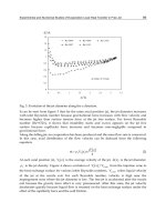
However, this method has limitations, as observed in Fig. 9, and in more details in Fig. 10.
The latter figure shows a close-up view of each of the 17 peaks of heat flux that happen
during the cooling process on the run-out table, i.e. the peaks in Fig. 9. The circles are the
expected heat flux, and the plusses are the result of NNs. The top left sub-figure is the first
peak heat flux in time, and then it moves to the right, and then to the next row. Note that
each even sub-figure (2nd, 4th, and so on) is a very smaller peak which is associated with the
second row of jets. These peaks are not very obvious in Fig. 9, due to the scaling. Going
through the subfigures of heat fluxes, it is apparent that the success or failure of NNs is not
that much related to the temperature range, or the magnitude of heat fluxes, but on the
actual shape of the heat flux profile. If the heat flux has a clear thin peak and two tails before
and after the peak, the NN is doing a good job. However, the existence of other details in the


52

Heat Conduction – Basic Research

heat flux profile reduces the quality of the NN predictions. Also, considering the ill-posed
nature of the problem, and all the complications that are involved, we can generally say that
in most cases (about 75% of the cases) it does a decent job. Of course, there is the possibility
of slightly improving the results by trying to modify the performance parameters of the NN,
but overall we can say that NNs are more useful in getting a general picture of the solution,
rather than producing a very accurate and detailed answer to the IHCP.
Expected

NN Results

25000000

20000000
15000000
10000000
5000000
0
-5000000

0

1

2

3

4

5

6

7

8

9

-10000000
-15000000
-20000000

Fig. 9. Time History of Heat Fluxes in a Typical Run-Out Table Application; Expected
Results (Squares) vs. the RBF Network Results (Line).

Fig. 10. Individual Heat Flux Peaks vs. Time from a Typical Run-Out Table Application;
Expected Results (Circles) vs. the RBF Network Results (Pluses)


Assessment of Various Methods in Solving Inverse Heat Conduction Problems

53

On the other hand, GA and PSO algorithms show reasonably good predictions of the details
of the missing boundary conditions. Notice that we still need to have some form of
regularization for these methods to work properly. The figures for the results of GA and
PSO are not presented here for the sake of brevity, but can be found in (Vakili & Gadala,
2009). They will be used, however, for comparisons in the next sections.
7.1 Time step size
One of the main problems of the classical approaches, such as the sequential function
specification method studied in this chapter, is their instability when small time steps are
used. Unlike direct problems where the stability requirement gives the upper limit of the
time step size, in inverse problems the time step is bounded from below. Fig. 11(a)(Vakili &
Gadala, 2009) shows the oscillation in the results obtained by the function specification
method and a time step size of 0.01 (s), which corresponds to the onset of instability. For
time steps smaller than this, the whole process diverges. PSO, GA, and NNs successfully
produce, however, the results for the same time step size as presented in Fig. 11(b) for PSO.
Note that the oscillations here are not due to the instability caused by the time step size, and
can be improved by performing more iterations. It is, however, important to mention that
the time requirements for these techniques are much higher than those of the classical
function specification approaches.

7.2 Efficiency
In this section, we compare the solution time required for GA, the three variations of PSO,
and feed forward and radial basis function neural networks. We assume that there is no
noise in the solution, and we compare the time that is required to get to certain accuracy in
the heat flux predictions. Table 1 compares the solution time for different inverse analysis
algorithms. The fastest solution technique is the gradient-based function specification
method. The stochastical methods such as GA and PSO variants suffer a high computational
cost. RBF neural networks perform much faster than GA and PSO, but they are still slower
than the gradient-based methods, such as function specification.

(a)

(b)

Fig. 11. Heat flux vs. time: (a) classical approach, (b) PSO (Vakili & Gadala, 2009).


54

Solution Time (s)

Heat Conduction – Basic Research

Function Specification
Method
1406

GA PSO RPSO CRPSO FMLP RBFN
8430 6189

5907

6136

7321

2316

Table 1. Comparison of the solution time for different inverse analysis algorithms.
A more detailed comparison between the efficiency of GA and PSO variations can be found
in (Vakili & Gadala, 2009).
7.3 Noisy domain solution
To investigate the behavior of different inverse algorithm variations in dealing with noise in
the data, a known boundary condition is first applied to the direct problem. The
temperature at some internal point(s) will be calculated and stored. Then random errors are
imposed onto the calculated exact internal temperatures with the following equation:
Tm  Texact    r

(22)

where Tm is the virtual internal temperature that is used in the inverse calculations instead
of the exact temperature, Texact; r is a normally distributed random variable with zero mean
and unit standard deviation; and σ is the standard deviation. Virtual errors of 0.1% and 1%
of the temperature magnitude are investigated here.
We start by studying the effectiveness of the neural networks in handling noisy domains.
Generally, the stability of the neural networks is on the same order as other inverse
methods. It may be possible to tune the parameters to make it a little bit more stable, but
generally it does not look promising in terms of noise resistance, since such modifications
exist for almost all other methods. Fig. 12 - Fig. 13 show the results of the RBF network

Fig. 12. Individual heat flux peaks vs. time from a typical run-out tale application; Expected
results (blue circles) vs. the RBF network results (red pluses); Artificial noise added: c = ±0.1%.


Assessment of Various Methods in Solving Inverse Heat Conduction Problems

55

(red pluses) versus the expected results (blue circles) for individual heat flux peaks during
the cooling history of the plate. The amount of added noise in these figures is ±0.1%and
±1%, respectively.
There are several ways to make an inverse algorithm more stable when dealing with noisy
data. For example, (Gadala & Xu, 2006) have shown that increasing the number of “future
time steps” in their sequential function specification algorithm resulted in greater stability.
They have also demonstrated that increasing the regularization parameter, α, improves the
ability of the algorithm to handle noisy data. However, the latter approach was shown to
greatly increase the required number of iterations, and in many cases the solution may
diverge. In this work, we first examine the effect of the regularization parameter, and then
investigate an approach unique to the PSO method, to improve the effectiveness of the
inverse algorithm in dealing with noise.
Fig. 14 shows the effect of varying the regularization parameter value on the reconstructed
heat flux, using the basic particle swarm optimization technique. Stable and accurate results
are obtained for a range of values of α = 10-12 to 10-10. These results are very close to those
reported in (Gadala & Xu, 2006), i.e., the proper values of α are very similar for the
sequential specification approach and PSO.

Fig. 13. Individual heat flux peaks vs. time from a typical run-out tale application;
Expected results (blue circles) vs. the RBF network results (red pluses); Artificial noise
added: c = ±1%.

56

Heat Conduction – Basic Research

Another factor that can affect the performance of a PSO inverse approach in dealing with
noisy data is the value of the self-confidence parameter, c0, or the ratio between this
parameter and the acceleration coefficients. The acceleration coefficients are set to the
default value of 1.42. The initial value of the self-confidence parameter, c0, is changed from
the default value of 0.7. The results are shown below.

(a)

(b)

Fig. 14. Effect of Regularization Parameter; a: α = 10-12; b: α = 10-10

(a)

Fig. 15. Effect of Self-Confidence Parameter; (a) c0=0.5; (b) c0=1.2

(b)


57

Assessment of Various Methods in Solving Inverse Heat Conduction Problems

As can be seen in Fig. 15 (for α = 10-10), increasing the value of the self-confidence
parameter results in better handling of the noisy data. This trend was observed for values

up to approximately 1.3, after which the results become worse, and diverge. One possible
explanation is that increasing the ratio of the self-confidence parameter with respect to the
acceleration coefficients results in a more global search in the domain, and therefore
increases the capability of the method to escape from the local minima caused by the
noise, and find values closer to the global minimum. This effect was observed to be
weaker in highly noisy domains. However, in the presence of a moderate amount of noise,
increasing the self-confidence ratio results in more effectiveness. As can be seen in Table 2,
the best effectiveness is normally obtained by RPSO, closely followed by CRPSO.
Considering the higher efficiency of CRPSO, it is still recommended for the inverse heat
conduction analysis.
C0
PSO
RPSO
CRPSO

0.7
8.105e+4
7.577e+4
7.611e+4

0.8
7.532e+4
7.064e+4
6.739e+4

0.95
7.079e+4
6.685e+4
6.117e+4

1.1
6.823e+4
6.346e+4
5.999e+4

1.2
6.257e+4
5.816e+4
5.822e+4

Table 2. Effect of the Self-Confidence Parameter on the L2 Norm of Error in the Solution
Table 3 shows the value of L2 norm of error in the solution, for ±1% added noise, and for
different algorithms. It can be seen that the RBF neural networks perform better than the
function specification method, and somewhere between the genetic algorithm and PSO
variants. The most noise resistant algorithms are PSO variants, and the least stable
algorithm is the gradient-based function specification method.
Function Specification
Method
L2 Norm of
Error

9.14e4

GA

PSO RPSO CRPSO FMLP RBFN

6.61e4 5.24e4 4.82e4

5.02e4

8.91e4 5.91e4

Table 3. The L2 Norm of Error in the Solution in a Noisy Domain for Different Algorithms
7.4 Effect of non-linearity
In many applications of inverse heat conduction, the thermophysical properties change
with temperature. This results in nonlinearity of the problem. In other words, a same drop
in the temperature values can be caused by different values of heat flux. So, a neural
network that is trained with the relationship between the temperature change values and
heat flux magnitudes may not be correctly capable of recognizing this nonlinear pattern,
and as a result the performance will suffer. To investigate this effect, two kinds of
expressions are used for thermal conductivity in this study. In one, we assume a constant
thermal conductivity of W/m.°C, while in the other a temperature-dependent expression
is used:
k  60.571  0.03849  T W/m.°C

(23)

As expected, the nonlinearity will weaken the performance of both feedforward and radial
basis function neural networks. The effect is seen as the training of the network stalls after a


58

Heat Conduction – Basic Research

number of epochs. In order to deal with this, increasing the number of hidden layers,
increasing the number of neurons in each layer, and choosing different types of transfer
function were investigated. However, none of these methods showed a significant
improvement in the behavior of the network. The other methods of solving the inverse

problem are much less sensitive to the effect of nonlinearity. Table 4 compares the error in
the solution for both the linear and nonlinear cases, if the same numbers of iterations,
generations, and epochs are used for different methods of solving the inverse heat
conduction. As it can be seen, the neural networks methods perform very poorly in the
nonlinear cases, while the other methods, either gradient based or stochastical, are immune
to the problems caused by nonlinearity. Basically, neural networks, at least in the form that
is used in this chapter, see nonlinearity as a kind of noise. It should be noted that neural
networks can be useful in making rough estimates of the answer, or combined with some
other techniques employed as an inverse solver for nonlinear cases (Aquino & Brigham,
2006), but on their own, are not a suitable choice for an accurate prediction of the boundary
conditions in a nonlinear inverse heat conduction problem.

Linear
Nonlinear

Function Specification
Method
1.81e2
2.14e2

GA

PSO RPSO CRPSO FMLP RBFN

7.62e2 3.85e2 3.42e2
7.71e2 4.46e2 5.12e2

3.17e2
4.26e2

9.90e2 5.35e2
3.57e4 2.76e4

Table 4. The L2 norm of error in the solution in an exact domain for different algorithms.

8. Conclusion
In this chapter, we introduced a gradient-based inverse solver to obtain the missing
boundary conditions based on the readings of internal thermocouples. The results show that
the method is very sensitive to measurement errors, and becomes unstable when small time
steps are used. Then, we tried to find algorithms that are capable of solving the inverse heat
conduction problem without the shortcomings of the gradient-based methods.
The artificial neural networks are capable of capturing the whole thermal history on the runout table, but are not very effective in restoring the detailed behavior of the boundary
conditions. Also, they behave poorly in nonlinear cases and where the boundary condition
profile is different.
GA and PSO are more effective in finding a detailed representation of the time-varying
boundary conditions, as well as in nonlinear cases. However, their convergence takes
longer. A variation of the basic PSO, called CRPSO, showed the best performance among the
three versions. The effectiveness of PSO was also studied in the presence of noise. PSO
proved to be effective in handling noisy data, especially when its performance parameters
were tuned. The proper choice of the regularization parameter helped PSO deal with noisy
data, similar to the way it helps the classical function specification approaches. An increase
in the self-confidence parameter was also found to be effective, as it increased the global
search capabilities of the algorithm. RPSO was the most effective variation in dealing with
noise, closely followed by CRPSO. The latter variation is recommended for inverse heat
conduction problems, as it combines the efficiency and effectiveness required by these
problems.


Assessment of Various Methods in Solving Inverse Heat Conduction Problems

59

9. References
Abou khachfe, R., and Jarny, Y. (2001). Determination of Heat Sources and Heat Transfer
Coefficient for Two-Dimensional Heat flow–numerical and Experimental Study.
International Journal of Heat and Mass Transfer, Vol. 44, No. 7 , pp.1309-1322.
Alifanov, O. M., Nenarokomov, A. V., Budnik, S. A., Michailov, V. V., and Ydin, V. M.
(2004). Identification of Thermal Properties of Materials with Applications for
Spacecraft Structures. Inverse Problems in Science and Engineering, Vol. 12, No. 5 ,
pp.579-594.
Alifanov, O.M., (1995). Inverse Heat Transfer Problems, Berlin ; New York: Springer-Verlag.
Al-Khalidy, N., (1998). A General Space Marching Algorithm for the Solution of TwoDimensional Boundary Inverse Heat Conduction Problems. Numerical Heat
Transfer, Part B, Vol. 34, , pp.339-360.
Alrasheed, M.R., de Silva, C.W., and Gadala, M.S. (2008).Evolutionary Optimization in the
Design of a Heat Sink, in: Mechatronic Systems: Devices, Design, Control, Operation
and Monitoring, C. W. de Silva, Taylor & Francis.
Alrasheed, M.R., de Silva, C.W., and Gadala, M.S. (2007).A Modified Particle Swarm
Optimization Scheme and its Application in Electronic Heat Sink Design,
ASME/Pacific Rim Technical Conference and Exhibition on Packaging and
Integration of Electronic and Photonic Systems, MEMS, and NEMS.
Aquino, W., and Brigham, J. C. (2006). Self-Learning Finite Elements for Inverse Estimation
of Thermal Constitutive Models. International Journal of Heat and Mass Transfer, Vol.
49, No. 15-16 , pp.2466-2478.
Bass, B. R., (1980). Application of the Finite Element Method to the Nonlinear Inverse Heat
Conduction Problem using Beck's Second Method. Journal of Engineering and
Industry, Vol. 102, , pp.168-176.
Battaglia, J. L., (2002). A Modal Approach to Solve Inverse Heat Conduction Problems.
Inverse Problems in Engineering, Vol. 10, No. 1 , pp.41-63.
Beck, J. V., Blackwell, B., and Haji-Sheikh, A. (1996). Comparison of some Inverse Heat
Conduction Methods using Experimental Data. International Journal of Heat and

Mass Transfer, Vol. 39, , pp.3649-3657.
Beck, J. V., and Murio, D. A. (1986). Combined Function Specification-Regularization
Procedure for Solution of Inverse Heat Conduction Problem. AIAA Journal, Vol. 24,
No. 1 , pp.180-185.
Beck, J.V., Blackwell, B., and Clair Jr, C.R.S. (1985). Inverse Heat Conduction: Ill-Posed Problem,
New York: Wiley-Interscience Publication.
Beck, J.V., and Arnold, K.J. (1977). Parameter Estimation in Engineering and Science, New York:
Wiley.
Blanc, G., Raynaud, M., and Chau, T. H. (1998). A Guide for the use of the Function
Specification Method for 2D Inverse Heat Conduction Problems. Revue Generale De
Thermique, Vol. 37, No. 1 , pp.17-30.
Clerc, M., (2006). Particle Swarm Optimization, ISTE.
Davis, L., (1991). Handbook of Genetic Algorithms, Thomson Publishing Group.


60

Heat Conduction – Basic Research

Eberhart, R., and Kennedy, J. (1995).A New Optimizer using Particle Swarm Theory,
Proceedings of the Sixth International Symposium on Micro Machine and Human
Science pp. 39-43.
Fan, S.K.S., and Chang, J.M. (2007).A Modified Particle Swarm Optimizer using an Adaptive
Dynamic Weight Scheme, in: Digital Human Modeling, V. G. Duffy, Springer Berlin
/ Heidelberg. pp. 56-65, .
Gadala, M. S., and Xu, F. (2006). An FE-Based Sequential Inverse Algorithm for Heat Flux
Calculation during Impingement Water Cooling. International Journal of Numerical
Methods for Heat and Fluid Flow, Vol. 16, No. 3 , pp.356-385.
Girault, M., Petit, D., and Videcoq, E. (2003). The use of Model Reduction and Function
Decomposition for Identifying Boundary Conditions of A Linear Thermal System.

Inverse Problems in Science and Engineering, Vol. 11, No. 5 , pp.425-455.
Goldberg, D.E., (1989). Genetic Algorithms in Search, Optimization and Machine Learning,
Addison-Wesley Longman Publishing Co., Inc. Boston, MA, USA.
Gosselin, L., Tye-Gingras, M., and Mathieu-Potvin, F. (2009). Review of Utilization of
Genetic Algorithms in Heat Transfer Problems. International Journal of Heat and Mass
Transfer, Vol. 52, No. 9-10 , pp.2169-2188.
Hassan, R., Cohanim, B., de Weck, O., and Venter, G. (2005).A Comparison of Particle
Swarm Optimization and the Genetic Algorithm, Proceedings of the 46th
AIAA/ASME/ASCE/AHS/ASC Structures, Structural Dynamics and Materials
Conference.
Huang, C. H., Yuan, I. C., and Herchang, A. (2003). A Three-Dimensional Inverse Problem
in Imaging the Local Heat Transfer Coefficients for Plate Finned-Tube Heat
Exchangers. International Journal of Heat and Mass Transfer, Vol. 46, No. 19 , pp.36293638.
Huang, C. H., and Wang, S. P. (1999). A Three-Dimensional Inverse Heat Conduction
Problem in Estimating Surface Heat Flux by Conjugate Gradient Method.
International Journal of Heat and Mass Transfer, Vol. 42, No. 18 , pp.3387-3403.
Karr, C. L., Yakushin, I., and Nicolosi, K. (2000). Solving Inverse Initial-Value, BoundaryValue Problems Via Genetic Algorithm. Engineering Applications of Artificial
Intelligence, Vol. 13, No. 6 , pp.625-633.
Karray, F.O., and de Silva, C.W. (2004). Soft Computing and Intelligent System Design - Theory,
Tools, and Applications, New York: Addison Wesley.
Kennedy, J., Eberhart, R.C., and Shi, Y. (2001). Swarm Intelligence, Morgan Kaufmann.
Kim, H. K., and Oh, S. I. (2001). Evaluation of Heat Transfer Coefficient during Heat
Treatment by Inverse Analysis. Journal of Material Processing Technology, Vol. 112, ,
pp.157-165.
Kim, S. K., and Lee, W. I. (2002). Solution of Inverse Heat Conduction Problems using
Maximum Entropy Method. International Journal of Heat and Mass Transfer, Vol. 45,
No. 2 , pp.381-391.
Krejsa, J., Woodbury, K. A., Ratliff, J. D., and Raudensky, M. (1999). Assessment of Strategies
and Potential for Neural Networks in the IHCP. Inverse Problems in Engineering, Vol.
7, No. 3 , pp.197-213.

Assessment of Various Methods in Solving Inverse Heat Conduction Problems

61

Kumagai, S., Suzuki, S., Sano, Y.R., and Kawazoe, M. (1995).Transient Cooling of Hot Slab
by an Impinging Jet with Boiling Heat Transfer, ASME/JSME Thermal Engineering
Conference pp. 347-352.
Lecoeuche, S., Mercere, G., and Lalot, S. (2006). Evaluating Time-Dependent Heat Fluxes
using Artificial Neural Networks. Inverse Problems in Science and Engineering, Vol.
14, No. 2 , pp.97-109.
Lee, K. H., Baek, S. W., and Kim, K. W. (2008). Inverse Radiation Analysis using Repulsive
Particle Swarm Optimization Algorithm. International Journal of Heat and Mass
Transfer, Vol. 51, , pp.2772-2783.
Louahia-Gualous, H., Panday, P. K., and Artioukhine, E. A. (2003). Inverse Determination of
the Local Heat Transfer Coefficients for Nucleate Boiling on a Horizontal Pipe
Cylinder. Journal of Heat Transfer, Vol. 125, , pp.1087-1095.
Osman, A. S., (1190). Investigation of Transient Heat Transfer Coefficients in Quenching
Experiments. Journal of Heat Transfer, Vol. 112, , pp.843-848.
Ostrowski, Z., R. A. Bialstrokecki, and A. J. Kassab. "Solving Inverse Heat Conduction
Problems using Trained POD-RBF Network Inverse Method." Inverse Problems in
Science and Engineering (2007).
Ozisik, M.N., (2000). Inverse Heat Transfer: Fundamentals and Applications, New York: Taylor
& Francis.
Pietrzyk, M., and Lenard, J. G. (1990). A Study of Heat Transfer during Flat Rolling.
International Journal of Numerical Methods in Engineering, Vol. 30, , pp.1459-1469.
Raudensky, M., Woodbury, K. A., Kral, J., and Brezina, T. (1995). Genetic Algorithm in
Solution of Inverse Heat Conduction Problems. Numerical Heat Transfer, Part B:
Fundamentals, Vol. 28, No. 3 , pp.293-306.

Roudbari, S., (2006). Self Adaptive Finite Element Analysis, Cornell University, .
Shiguemori, E. H., Da Silva, J. D. S., and De Campos Velho, H. F. (2004). Estmiation of Initial
Condition in Heat Conduction by Neural Networks. Inverse Problems in Science and
Engineering, Vol. 12, No. 3 , pp.317-328.
Silieti, M., Divo, E., and Kassab, A. J. (2005). An Inverse Boundary Element method/genetic
Algorithm Based Approach for Retrieval of Multi-Dimensional Heat Transfer
Coefficients within Film Cooling holes/slots. Inverse Problems in Science and
Engineering, Vol. 13, No. 1 , pp.79-98.
Urfalioglu, O., (2004).Robust Estimation of Camera Rotation, Translation and Focal Length
at High Outlier Rates, The First Canadian Conference on Computer and Robot
Vision pp. 464-471.
Vakili, S., and Gadala, M. S. (2011). A Modified Sequential Particle Swarm Optimization
Algorithm with Future Time Data for Solving Transient Inverse Heat Conduction
Problems. Numerical Heat Transfer, Part A: Applications, Vol. 59, No. 12 , pp.911933.
Vakili, S., and Gadala, M. S. (2010). Boiling Heat Transfer of Multiple Impinging Round Jets
on a Hot Moving Plate. Submitted to Heat Transfer Engineering .
Vakili, S., and Gadala, M. S. (2009). Effectiveness and Efficiency of Particle Swarm
Optimization Technique in Inverse Heat Conduction Analysis. Numerical Heat
Transfer, Part B: Fundamentals, Vol. 56, No. 2 , pp.119-141.


62

Heat Conduction – Basic Research

Woodbury, K. A., and Thakur, S. K. (1996). Redundant Data and Future Times in the Inverse
Heat Conduction Problem. Inverse Problems in Science and Engineering, Vol. 2, No. 4 ,
pp.319-333.

0
3
Identifiability of Piecewise Constant Conductivity
Semion Gutman1 and Junhong Ha2
2 Korea

1 University

of Oklahoma
University of Technology and Education
2 South

1 USA

Korea

1. Introduction
Consider the heat conduction in a nonhomogeneous insulated rod of a unit length, with the
ends kept at zero temperature at all times. Our main interest is in the identification and
identifiability of the discontinuous conductivity (thermal diffusivity) coefficient a( x ), 0 ≤
x ≤ 1. The identification problem consists of finding a conductivity a( x ) in an admissible set
K for which the temperature u ( x, t) fits given observations in a prescribed sense.
Under a wide range of conditions one can establish the continuity of the objective function
J ( a) representing the best fit to the observations. Then the existence of the best fit to data
conductivity follows if the admissible set K is compact in the appropriate topology. However,
such an approach usually does not guarantee the uniqueness of the found conductivity a( x ).
Establishing such a uniqueness is referred to as the identifiability problem. For an extensive
survey of heat conduction, including inverse heat conduction problems see (Beck et al., 1985;
Cannon, 1984; Ramm, 2005)
From physical considerations the conductivity coefficients a( x ) are assumed to be in

Aad = { a ∈ L ∞ (0, 1) : 0 < ν ≤ a( x ) ≤ μ }.

(1)

The temperature u ( a) = u ( x, t; a) inside the rod satisfies
u t − ( a( x )u x ) x = f ( x, t),
Q = (0, 1) × (0, T ),
u (0, t) = q1 (t), u (1, t) = q2 (t), t ∈ (0, T ),
u ( x, 0) = g( x ),
x ∈ (0, 1),

(2)

where g ∈ H = L2 (0, 1), q1 , q2 ∈ C1 [0, ∞ ). Suppose that one is given an observation z(t) =
u ( p, t; a) of the heat conduction process (2) for t1 < t < t2 at some observation point 0 < p <
1. From the series solution for (2) and the uniqueness of the Dirichlet series expansion (see
Section 5), one can, in principle, recover all the eigenvalues of the associated Sturm-Lioville
problem. If one also knows the eigenvalues for the heat conduction process with the same
coefficient a and different boundary conditions, then classical results of Gelfand and Levitan
(Gelfand & Levitan, 1955) show that the conductivity a( x ) can be uniquely identified from the
knowledge of the two spectral sequences.
Alternatively, the conductivity is identifiable if the entire spectral function is known (i.e. the
eigenvalues and the values of the derivatives of the normalized eigenfunctions at x = 0).
However, such results have little practical value, since the observation data z(t) always