Ozone Reaction Kinetics for Water and Wastewater Systems - Chapter 4 ppt
Bạn đang xem bản rút gọn của tài liệu. Xem và tải ngay bản đầy đủ của tài liệu tại đây (812.8 KB, 22 trang )
©2004 CRC Press LLC
4
Fundamentals
of Gas–Liquid
Reaction Kinetics
The kinetics of heterogeneous reactions is governed by absorption theories of gases
in liquids accompanied by chemical reactions. The fundamentals of these theories
are necessary to understand the phenomena developing during the ozonation of
compounds in water. The necessary steps to study the kinetics of gas–liquid reactions
are described below. Since ozone reactions can be considered irreversible, isothermic,
and of second order
1
(for a general ozone–B reaction) or pseudo first-order (a case
of ozone decomposition reaction), the discussion that follows mainly refers to this
type of gas–liquid reactions. Nonetheless, some fundamental aspects on series-
parallel reactions are also given. Notice that ozonation of compounds in water yields
a series of by-products that also react with ozone. Therefore, the kinetics of series-
parallel gas–liquid reactions constitutes another part of this study. As a first step,
the physical absorption of a gas in a liquid is treated as commented below.
4.1 PHYSICAL ABSORPTION
In a gas–liquid reacting system, diffusion, convection, and chemical reaction proceed
simultaneously, and the behavior of the system can be predicted with the use of
models that simulate the situation for practical purposes. These models are based
on those describing the gas physical absorption phenomena, that is, they are based
on gas absorption theories. In a general case, when gas and liquid phases are in
contact, the components of one phase can transfer to the other to reach the equilib-
rium. If it is assumed that one component A of a gas phase is transferred to the
liquid phase, the rate of mass transfer or absorption rate of A is as follows:
(4.1)
where SI units of
N
A
are in molm
–2
s
–1
,
k
G
and
k
L
are the individual mass transfer
coefficients for the gas and liquid phases, respectively;
P
Ab
and
P
i
the partial pres-
sures of A in the bulk gas and at the interface, respectively; and
C
A
*
and
C
Ab
, are
the concentrations of A at the interface and in the bulk of the liquid, respectively
(see Figure 4.1). One of the two problems of the rate law is to find some mathematical
expression for the mass transfer coefficients. The other one is to know the interfacial
concentrations,
P
i
or
C
A
*
. Theoretical expressions for mass transfer coefficients
NkPPkCC
AG
Ab
iLA
Ab
=−
()
=−
()
*
©2004 CRC Press LLC
can be found from the solution of the microscopic mass balance equation of the
transferred component A that, applied to the liquid phase, is as follows:
(4.2)
where the term on the left side represents the molecular and turbulent transport rate
of
A
and the first and second ones on the right side represent the terms of convection
and accumulation rates of
A
, respectively. Equation (4.2) is conveniently simplified
according to the hypothesis of the absorption theories. The most applied absorption
theories are: the film and surface renewal theories.
4.1.1 T
HE
F
ILM
T
HEORY
Lewis and Withman
2
proposed that when two nonmiscible phases are in contact, the
main resistance to mass transfer is located in a stationary layer of width
δ
closed to
the interface, called the film layer. It is also assumed that mass transfer through the
film is only due to diffusion and that the concentration profiles with distance to the
interface are reached instantaneously. It is then called a theory of the pseudo sta-
tionary state.
In a gas–liquid system there will be two films, one for each phase. In most
common situations the gas is bubbled into the liquid phase, so the interfacial surface
is due to the external surface of bubbles. Concentration profiles of the gas component
being absorbed for both the gas and liquid films are as shown in Figure 4.2. The
film theory assumes a plane interfacial surface when the bubble radius is much lower
than the film thick,
δ
, a situation fulfilled in most of the gas–liquid systems. Accord-
ing to these statements (diffusion, stationary state, and one direction for mass
transfer), Equation (4.2) reduces to:
(4.3)
FIGURE 4.1
Concentration profile of a gas component A with the distance to the interface
during its physical absorption in a liquid.
Gas phase
P
Ab
C
A
*
P
i
C
Ab
0
x
, distance to interface
Liquid phase
Gas–liquid
interface
DCUC
C
t
TA A
A
∇=∇+
∂
∂
2
D
C
x
A
A
∂
∂
=
2
2
0
©2004 CRC Press LLC
Equation (4.3) can be solved with the following conditions:
(4.4)
where
δ
L
and
C
Ab
are the liquid film layer and concentration of A in bulk liquid,
respectively. Solution to this mathematical model leads to the concentration profile
of
A
:
(4.5)
By application of Fick’s law, the rate of mass transfer or absorption rate is:
(4.6)
Notice that a similar expression could be obtained for the gas phase if the microscopic
Equation (4.3) is applied to the gas film layer. Comparing Equation (4.6) with the
general Equation (4.1), the film theory yields the following equation for
k
L
:
(4.7)
Thus,
δ
L
, the width of film, is the characteristic parameter of film theory.
FIGURE 4.2
Concentration profile of a gas component A with the distance to the interface
during its physical absorption according to the film theory.
0
x
P
Ab
C
Ab
P
i
C
A
*
δ
G
δ
L
Gas–liquid
interface
Gas phase
Bulk gas Gas film Liquid film Bulk liquid
Liquid phase
xCC
xCC
AA
LA
Ab
==
==
0
*
δ
CC
CC
AA
A
Ab
L
=−
−
*
*
δ
ND
dC
dx
D
CC
Ao A
A
x
A
L
A
Ab
=− = −
()
=0
δ
*
k
D
L
A
L
=
δ
©2004 CRC Press LLC
4.1.2 S
URFACE
R
ENEWAL
T
HEORIES
In these models, the liquid is assumed to be formed by elements of infinite width
that are exposed to the interface for a given time and then are replaced by other
elements coming from the bulk liquid. While the liquid elements are at the interface,
mass transfer occurs by diffusion in a nonstationary way. The most-used surface
renewal theory is that proposed by Danckwerts
3
which assumes a distribution func-
tion of exposition times for the liquid elements. For this surface renewal theory,
Equation (4.2) reduces to the following one:
(4.8)
with the boundary limits:
(4.9)
After application of Fick’s law,
4
once the concentration profile of A with time and
position [
C
A
=
f
(
x
,
t
)] has been determined from the solution of Equation (4.8), the
mean absorption rate of
A
is as follows:
(4.10)
where
N
A
(
t
) is the absorption rate at
x
= 0 and
ψ
(
t
) is the distribution function for
exposition times of liquid elements, defined as
3
:
(4.11)
and
s
is the surface renewal velocity of any element, parameter that characterizes
the Danckwerts theory.
If Equation (4.10) and Equation (4.1) are compared, the mass transfer coefficient
k
L
is defined as:
(4.12)
4.2 CHEMICAL ABSORPTION
When the gas component
A
, being absorbed simultaneously, undergoes a chemical
reaction in the liquid, the microscopic mass balance Equation (4.2) presents an
additional term due to the chemical reaction rate law,
r
A
:
D
C
x
C
t
A
AA
∂
∂
=
∂
∂
2
2
tCC
txCC
xCC
A
Ab
AA
A
Ab
==
>= =
→∞ =
0
00
*
NNttdtDsCC
AA AA
Ab
==−
()
∞
∫
() ()
*
ψ
0
ψ() exp( )ts st=−
kDs
LA
=
©2004 CRC Press LLC
(4.13)
This is the case of the ozonation reactions. Determination of the gas absorption rate
(or ozonation rate for ozone processes) also requires following the steps shown above
for the case of physical absorption, that is:
• Solving the microscopic differential mass balance equation to find out the
concentration profile of the gas being absorbed with distance to the interface
• The application of Fick’s law to yield the gas absorption rate
Solution of the mass balance Equation (4.13) depends on the absorption theory
applied as explained below for the film and Danckwerts theories. The cases that are
treated correspond to irreversible first- (or pseudo first-) and second-order reactions
which are usually the case of simple ozonation reactions in water.
4.2.1 F
ILM
T
HEORY
4.2.1.1 Irreversible First-Order or Pseudo First-Order Reactions
This is the case of reactions with the following stoichiometry:
1. First-order reaction:
(4.14)
with
(4.15)
2. Pseudo first-order reaction:
(4.16)
with
(4.17)
The ozone self-decomposition reaction in water is the typical example that follows
this kinetics.
According to the film theory, the mass balance Equation (4.13) becomes:
(4.18)
DCrUC
C
t
TAA A
A
∇+=∇+
∂
∂
2
AP
k
1
→
rkC
AA
=−
1
AzB P
k
+→
′
1
rkCCkC
AABA
=−
′
=
11
D
C
x
kC
A
A
A
∂
∂
=
2
2
1
©2004 CRC Press LLC
being solved with the boundary conditions given in Equation (4.4). Solution of this
system leads to the following concentration profile of
A
with the distance to the
interface:
(4.19)
where
Ha
1
is called the dimensionless number of Hatta for an irreversible first-order
reaction defined as follows:
(4.20)
The square of
Ha
1
represents the ratio between the maximum chemical reaction rate
through the film layer and the maximum physical absorption rate:
(4.21)
where a is the specific interfacial area and
k
L
a
the volumetric mass transfer coefficient
in the liquid phase. Notice that the product
a
δ
L
is the ratio between the liquid film
and liquid total volumes. Thus,
Ha
1
indicates the relative importance of chemical
reaction and mass transfer rates in the gas liquid system.
Application of Fick’s law at the gas–liquid interface leads to the gas absorption
rate equation, or to the rate or kinetic law for this type of reaction:
(4.22)
where
M
1
is the maximum physical absorption rate,
k
L
C
A
*
is expressed per unit of
interfacial surface. Notice that in Equation (4.21), the maximum physical absorption
rate is expressed per unit of volume.
In Equation (4.22), it is convenient to express C
Ab
as a function of chemical and
mass transfer parameters. Then, the mass transfer rate at the other edge of the film
layer, (x = δ
L
), N
Aδ
, and the chemical reaction rate in the bulk of the liquid, R
b1
, are
needed:
(4.23)
and
CC
x
Ha
Ha
C
x
Ha
Ha
AA
L
Ab
L
=
−
+
*
sinh
sinh
sinh
sinh
1
1
1
1
1
δδ
Ha
kD
k
A
L
1
1
=
Ha
kC a
kaC
AL
LA
1
2
1
=
*
*
δ
ND
dC
dx
M
Ha
tahnHa
C
CHa
Ao A
A
x
Ab
A
=− = −
=0
1
1
11
1
1
*
cosh
NN M
Ha
Ha
C
C
Ha
A
A
x
Ab
A
L
δ
δ
== −
=
1
1
1
1
1
sinh
cosh
*
©2004 CRC Press LLC
(4.24)
where units of both rates are given per surface of interfacial area, β being the liquid
hold-up, it is defined as the ratio of liquid to total (gas plus liquid) volumes.
By equalizing Equation (4.23) and Equation (4.24), the ratio between concen-
trations of A in the bulk of the liquid and at the interface, C
Ab
/C
A
*
, can be obtained.
Then, after substitution in Equation (4.22), Equation (4.25) is obtained:
(4.25)
Also, if C
Ab
/C
A
*
is expressed as a function of β/aδ
L
, a dimensionless number that
represents the ratio between the volumes of the total liquid (film plus bulk liquids)
and film layer, the following alternative equation is obtained
5
:
Equation (4.25) or Equation (4.26) constitute the general kinetic equations for first-
order (or pseudo first-order) gas–liquid reactions.
As can be deduced from Equation (4.25), the absorption rate is a function of
three maximum rates:
• R
b1
maximum chemical reaction rate in the bulk liquid = k
1
C
Ab
β/a
• M
1
maximum physical absorption rate at the interface = k
L
C
A
*
• R
F
maximum chemical reaction rate through the film layer = k
1
C
A
*
aδ
L
Also, depending on the values of Ha
1
, the absorption rate develops in different kinetic
regimes
6
:
• The fast kinetic regime when Ha
1
> 3, then C
A0
= 0 with:
(4.27)
• The moderate kinetic regime when 3 < Ha
1
< 0.3 with the general Equation
(4.25) or Equation (4.26)
RkC
a
bAb1
1
=
β
ND
dC
dx
M
Ha
tanhHa
M
Ha
Ha Ha
RM
Ha
tanhHa
Ao A
A
x
b
=− = −
+
=0
1
1
1
1
1
11
1
1
1
1
1
sinh cosh
(4.26)
NMHa
Ao
=
11
©2004 CRC Press LLC
• The diffusional kinetic regime when Ha
1
< 0.3 and C
Ab
= 0 with:
(4.28)
• The slow kinetic regime when Ha
1
< 0.3 and C
Ab
≠ 0 with the general
Equation (4.25) or Equation (4.26)
• The very slow kinetic regime when Ha
1
Ӷ 0.01 with :
(4.29)
As can be deduced, depending on the relative importance of mass transfer and
chemical reaction rates, the kinetics of the gas–liquid reaction will be the chemical
reaction rate (the case of very slow kinetic regime) or the physical absorption rate
(slow and diffusional regimes). Notice that for slow kinetic regimes, the gas–liquid
reaction is a two-series process where mass transfer through the film layer first
occurs and then the chemical reaction develops in the bulk liquid. Then, the absorp-
tion rate equation is also:
(4.30)
Since the general Equation (4.25) is rather complex, the absorption rate is usually
expressed as a function of another dimensionless number called reaction factor E:
(4.31)
As deduced from Equation (4.31), the reaction factor can be defined as the number
of times the maximum physical absorption rate increases due to the chemical reac-
tion. Notice that this definition has only physical meaning when the kinetic regime
is fast or moderate, (for C
Ab
= 0). However, according to Equation (4.31), values of
E can be lower than unity (the cases of slow kinetic regime or some others with
moderate regime), although they have no practical use. In Figure 4.3, a plot of E
against Ha
1
is shown with the zones of different kinetic regimes. Notice that for a
slow kinetic regime (Ha
1
< 0.3) Equation (4.26) is used to show the variation of E
with the Hatta number. This is because, in the slow kinetic regime, reactions develop
in the bulk liquid and the volume ratio parameter β/aδ
L
has a great influence on the
gas absorption rate.
4.2.1.2 Irreversible Second-Order Reactions
These constitute the typical case of most of ozone direct reactions in water. The
stoichiometric equation is:
(4.32)
NM
Ao
=
1
NR
Ao
b
=
1
NkCC R
Ao L A
Ab b
=−
()
=
*
1
E
N
M
Ao
=
1
AzB P
k
+→
2
©2004 CRC Press LLC
and the chemical reaction rate referred to the disappearance of A:
(4.33)
For this case, both microscopic mass balance equation of A and B have to be simul-
taneously solved:
(4.34)
(4.35)
Boundary conditions of this mathematical model are:
(4.36)
However, it is not possible to find out any analytical solution to this system. Van
Krevelen and Hoftijzer
7
found an approximate solution by assuming that the con-
centration of B through the reaction zone in the film layer is constant, C
Br
, so that
the system transforms to a pseudo first-order one. Figure 4.4 shows the concentration
profiles of the actual and assumed situations. In this way, the rate equations deduced
in Section 4.2.1.1 could be applied with k
1
= k
2
C
Br
. By applying the proposed
approximation,
7
the following equation was found for C
Br
:
(4.37)
FIGURE 4.3 Variation of the reaction factor with the Hatta number for one irreversible first-
or pseudo first-order gas liquid reaction.
E
10
2
10
2
10
1
10
–1
10
–2
10
–3
10
–4
10
–5
10
–5
10
–4
10
–3
10
–2
10
–1
10
1
10
2
10
–6
10
–7
10
–8
10
–9
10
–10
1
1
Hatta number
β/aδ
L
=10
6
β/aδ
L
=10
3
β/aδ
L
=1
E
= Ha
Fast reaction zone
Slow reaction zone
rkCC
AAB
=−
2
D
C
x
kCC
A
A
AB
∂
∂
=
2
2
2
D
C
x
zk C C
B
A
AB
∂
∂
=
2
2
2
xCC
dC
dx
xCCCC
AA
B
LA
Ab
B
Bb
== =
== =
00
*
δ
CC E
zC
C
Br
Bb
A
Bb
=−−
11()
*
©2004 CRC Press LLC
Then Ha
1
[see Equation (4.20)] becomes
(4.38)
Equation (4.38) can be simplified to Equation (4.39):
(4.39)
where Ha
2
represents the Hatta number of the irreversible second order reaction
(4.32) and has the same physical meaning as Ha
1
in Equation (4.20):
(4.40)
Finally, the absorption rate of A accompanied by an irreversible second order
chemical reaction with B is given by Equation (4.25) with Ha
1
given by Equation
(4.39). The system is solved with Equation (4.31) by a trial-and-error procedure that
allows the values of the reaction factor E to be obtained from the values of Ha
2
.
The solution is usually presented in plots such as Figure 4.5. As deduced from
Equation (4.25) and Equation (4.38), the absorption rate is a function of four
maximum rates (three of them previously deduced for the first order reaction kinetics)
defined as follows:
FIGURE 4.4 Concentration profiles of a gas component A and one liquid component B with
the distance to the gas–liquid interface during their fast chemical reaction while A is diffusing
through the liquid film. Profiles of B concentration according to the film theory: continuous
line; profiles of B concentration according to the simplification of Van Krevelen and Hoftijzer
7
:
dotted line. (From Van Krevelen, D.W. and Hoftijzer, P.J., Kinetics of gas liquid reactions.
Part I. General theory, Rec. Trav. Chim., 67, 563–586, 1948. With permission.)
Gas–liquid
interface
Liquid phase
Liquid film Bulk liquid
0
δ
L
x
C
A
*
x
R
C
Bi
C
Bb
C
BR
Reaction zone
0 < x < x
R
Ha
kDC
k
kDC
k
E
zC
C
ABr
L
A
Bb
L
A
Bb
1
2
2
11== −−()
*
Ha Ha E
zC
C
A
Bb
12
11=−−()
*
Ha
kDC
k
A
Bb
L
2
2
=
©2004 CRC Press LLC
• R
b2
maximum chemical reaction rate in the bulk liquid:
(4.41)
• M
1
maximum physical absorption rate at the interface = k
L
C
A
*
• R
F
maximum chemical reaction rate through the film layer:
(4.42)
• M
2
maximum physical diffusion of B through the film layer:
(4.43)
For the case of second order reaction there are two new kinetic regimes to consider
in addition to those listed for first order reactions:
•Fast kinetic regime, with C
Ab
= 0 and Ha
2
> 3:
(4.44)
where Ha
1
is given by Equation (4.38)
• Instantaneous kinetic regime with C
A0
= 0 and Ha
2
> 10E
i
:
(4.45)
where E
i
is the reaction factor for the instantaneous reaction, defined as
follows:
FIGURE 4.5 Variation of the reaction factor with the Hatta number for one irreversible
second-order gas liquid reaction.
10
3
10
2
10
1
10
–1
10
1
10
2
10
3
E
= Ha
E
i
= 1000
E
i
= 500
E
i
= 100
E
i
= 50
E
i
= 10
E
i
= 5
1
1
E
Hatta number
RkCC
a
b
A
Bb2
2
=
*
β
RkCCa
FA
Bb
L
=
2
*
δ
M
z
kC
L
Bb
2
1
=
NkC
Ha
Ha
ALA0
1
1
=
*
tanh
NkCE
ALAi0
=
*
©2004 CRC Press LLC
(4.46)
where D
B
is the diffusivity of compound B in the liquid that can be estimated
with the equation of Wilke and Chang
8,9
as indicated in Section 5.1.1.
Notice that the fast kinetic regime for first order reaction is now called the fast
pseudo first-order kinetic regime with the following condition to be fulfilled:
(4.47)
The absorption rate law being in this case:
(4.48)
Figure 4.6 to Figure 4.12 show the concentration profiles of A and B through the
liquid that hold for the different kinetic regimes. Notice that for fast or instantaneous
kinetic regimes, the chemical reaction develops in a zone or plane of the film layer,
respectively, while for slow kinetic regimes, the chemical reaction is in the bulk
liquid. Also notice that for fast or instantaneous kinetic regime there will not be
dissolved gas in the bulk liquid (C
Ab
= 0). It should be highlighted that the rate
equations presented are per unit of interfacial surface area (that is in mols
–1
m
–2
). In
a practical situation, the problem is that the interfacial surface area is generally
unknown. Nonetheless, this problem is overcome by multiplying both sides of the
absorption rate equation by the specific interfacial area, a, so that the rate will be
given per unit of volume which is known. It should also be reminded that depending
on the relative importance of mass transfer and chemical reaction steps, that is,
depending on the kinetic regime, the general Equation (4.25), once Equation (4.38)
has been accounted for, simplifies in a similar way as shown for the case of first
order reaction. These simplifications will be used in the kinetic study of water
ozonation reactions as shown later.
4.2.1.3 Series-Parallel Reactions
In most cases, ozone reacts not only with the compound initially present in water
but also with the intermediate compounds formed in a series-parallel reaction system.
Thus, a simplified study of the kinetics (absorption rate law) of these gas–liquid
systems is presented here. For so doing, let us assume that a gas component A
transfers into the liquid where it undergoes the following reactions:
(4.49)
(4.50)
E
DC
zD C
i
B
Bb
AA
=+1
*
3
2
2
23
<= <Ha
kD C
k
E
O
Bb
L
i
NaCkDC
AAO
Bb
023
=
*
AzB zC
b
k
c
+→
1
AzC zD
c
k
d
+
′
→
2
©2004 CRC Press LLC
FIGURE 4.6 Film theory: very slow kinetic regime. Concentration profiles for A (gas being
dissolved) and B (liquid component) with the distance to the interface.
FIGURE 4.7 Film theory: slow kinetic regime. Concentration profiles for A (gas being
dissolved) and B (liquid component) with the distance to the interface.
FIGURE 4.8 Film theory: diffusional kinetic regime. Concentration profiles for A (gas being
dissolved) and B (liquid component) with the distance to the interface.
Gas–liquid
interface
Liquid phase
Liquid film Bulk liquid
0
δ
L
x
C
A
*
C
Bi
C
Bb
C
Ab
Reaction zone
x
> δ
L
Gas–liquid
interface
Liquid phase
Liquid film Bulk liquid
0
δ
L
x
C
A
*
C
Bi
C
Bb
C
Ab
Reaction zone
x
> δ
L
Gas–liquid
interface
Liquid phase
Liquid film Bulk liquid
0
δ
L
x
C
A
*
C
Bi
C
Bb
C
Ab
Reaction zone
x
> δ
L
=0
©2004 CRC Press LLC
Solution of this system requires the microscopic balance the equation of A, B, and
C compounds that, in a general form, are represented in Equation (4.51):
(4.51)
with the following conditions:
(4.52)
where C
Bi
and C
Ci
are the concentrations of B and C at the interface.
FIGURE 4.9 Film theory: moderate kinetic regime. Concentration profiles for A (gas being
dissolved) and B (liquid component) with the distance to the interface.
FIGURE 4.10 Film theory: fast (general) kinetic regime. Concentration profiles for A (gas
being dissolved) and B (liquid component) with the distance to the interface.
Two possible cases:
Gas–liquid
interface
Liquid phase
Liquid film
Bulk liquid
0
δ
L
x
C
A
*
C
Bi
C
Bb
Reaction zone
x > 0
C
Ab
=0 or C
Ab
≠0
Gas–liquid
interface
Liquid phase
Liquid film Bulk liquid
0
δ
L
x
C
A
*
C
Bi
C
Bb
C
Ab
Reaction zone
0 < x
< δ
L
=0
D
dC
dx
r
i
i
i
2
2
0+=
xCCCCCC
dC
dx
dC
dx
xCCCCCC
AABBiCCi
B
C
LA
Ab
B
Bb
C
Cb
== = = = =
== = =
000
*
δ
©2004 CRC Press LLC
Onda et al.
10
found an expression for the reaction factor, E, [Equation (4.53)]
after introducing a series of approximations based on that of Van Krevelen and
Hoftijzer
7
:
(4.53)
where
(4.54)
and Ha
2
being now the Hatta number of reaction (4.49). As observed, solution of
the mathematical model requires C
bi
and C
ci
be known. Onda et al.
10
applied another
FIGURE 4.11 Film theory: fast of pseudo first-order kinetic regime. Concentration profiles
for A (gas being dissolved) and B (liquid component) with the distance to the interface.
FIGURE 4.12 Film theory: instantaneous kinetic regime. Concentration profiles for A (gas
being dissolved) and B (liquid component) with the distance to the interface.
Gas–liquid
interface
Liquid phase
Liquid film Bulk liquid
0
δ
L
x
C
A
*
C
Bi
C
Bb
C
Ab
Reaction zone
0 < x
< δ
L
=0
Gas–liquid
interface
Liquid phase
Liquid film Bulk liquid
0 x
R
δ
L
x
C
A
*
C
Bb
Reaction zone
x
=
x
R
E
Ha
Ha
C
C
Ha
s
s
Ab
A
s
=−
tanh
senh
*
1
Ha Ha
C
C
kC
kC
s
Bi
Bb
Ci
Cb
=+
2
2
2
1
©2004 CRC Press LLC
equation for the reaction factor, obtained from a total molar balance in differential
form:
(4.55)
On the other hand, after application of some hypothesis related to the concentration
profiles of B and C through the film layer, the following equation that relates the
concentration of both compounds was found
10
:
(4.56)
Finally, a trial and error procedure allows the determination of C
bi
and C
ci
and the
reaction factor E. As it was shown for simple first or second order reactions (see
Figure 4.3 and Figure 4.5), solution of E at different conditions (that is, at different
Ha
2
) is usually found in plots with k
2
/k
1
as parameter as literature reports.
10
4.2.2 DANCKWERTS SURFACE RENEWAL THEORY
4.2.2.1 First-Order or Pseudo First-Order Reactions
For the system where reaction (4.14) develops, the starting microscopic mass balance
equation of A in the liquid is now:
(4.57)
that should be solved with the boundary conditions (4.9). Danckwerts
11
found an
analytical solution for the case of fast reactions (C
Ab
= 0) and Ha
1
> 1:
(4.58)
4.2.2.2 Irreversible Second-Order Reactions
For the kinetics of the second-order gas–liquid reaction (4.32), the case of instan-
taneous kinetic regime was first solved. For this case, the microscopic mass balance
equation of A and B are:
(4.59)
E
C
C
D
zD
z
z
C
C
D
zD
C
C
C
C
Ab
A
B
b
A
c
c
Bi
Bb
C
cA
Bb
A
Ci
Cb
=− + +
′
−
−
′
+111
**
C
C
C
C
zD
zD
C
C
zD
zD
k
k
C
C
C
C
Ci
Bi
cb
Bb
cB
b
C
Bi
Bb
cB
b
C
Bi
Bb
Bi
Bb
=
+−
+
′
−
1
1
5
6
1
2
1
D
C
x
C
t
kC
A
AA
A
∂
∂
=
∂
∂
+
2
2
1
NkC Ha
ALA01
2
1=+
*
D
C
x
C
t
A
AA
∂
∂
=
∂
∂
2
2
©2004 CRC Press LLC
(4.60)
that can be solved with the following boundary conditions:
(4.61)
with x
i
being the distance to the interface where A and B react instantaneously (in
a reaction plane, see Figure 4.12). This parameter, x
i
, has to fulfill equation (4.62)
11
:
(4.62)
where β is found by trial and error from equation (4.63):
(4.63)
Thus, solving the mathematical system, the following concentration profiles of A
and B can be found:
(4.64)
(4.65)
and, then, the absorption rate law is obtained after the application of Ficks law and
the exposition time distribution function [see Equation (4.11)]:
(4.66)
D
C
x
C
t
B
BB
∂
∂
=
∂
∂
2
2
xCC
xxC C
xCC
AA
iA B
B
Bb
==
===
→∞ =
0
0
*
xt
i
= 2β
exp exp
*
ββββ
22
D
erfc
D
C
zC
D
DD
erfc
D
BB
Bb
A
B
AA A
=
CC
erf
x
Dt
erfc
D
erf
D
for x x
AA
AA
A
i
=
−
≤
*
2
χ
χ
CC
erf
x
Dt
erfc
D
erf
D
for x x
B
Bb
BA
A
i
=
−
≥
2
χ
χ
NkC
erf
D
ALA
A
0
1
=
*
χ
©2004 CRC Press LLC
From the definition of reaction factor or equation (4.31), the instantaneous reaction
factor is here defined as:
(4.67)
In many cases, Equation (4.67) can be simplified to the more known equation (4.68):
(4.68)
which is valid when
(4.69)
Also notice that E
i
from Equation (4.68) coincides with that of the film theory
[Equation (4.46)] when D
A
= D
B
.
If the kinetic regime is not instantaneous, the starting microscopic mass balance
equations of A and B with the appropriate boundary conditions are:
(4.70)
(4.71)
that can be solved with the following boundary conditions:
(4.72)
An approximate analytical solution to the mathematical model of Equation (4.70)
and Equation (4.71) has only been found for the case of fast kinetic regime. Thus,
DeCoursey
12
arrived at the following absorption rate law:
(4.73)
E
erf
D
i
A
=
1
χ
E
D
D
CD
zC D
i
A
B
Bb
B
AA
=+
1
*
C
zC
Bb
A
*
> 25
D
C
x
C
t
kCC
A
AA
AB
∂
∂
=
∂
∂
+
2
2
2
D
C
x
C
t
zk C C
A
AB
AB
∂
∂
=
∂
∂
+
2
2
2
tCCCC
txCC
dC
dx
xCCCC
A
Ab
B
Bb
AA
B
A
Ab
B
Bb
== =
>= = =
→∞ = =
0
00 0
*
NM Ha
EE
E
MM
A
i
01 2
2
1
1
1
1
1=+
−
−
=+
′
©2004 CRC Press LLC
As a difference from the film theory [see Equation (4.25) and Equation (4.38)],
Equation (4.73) allows the reaction factor E to be determined in an explicit way:
(4.74)
4.2.2.3 Series-Parallel Reactions
The theory of Danckwerts has also been used to explain the kinetics of series-parallel
reaction systems such as that of reactions (4.49) and (4.50). Also in this case,
approximate and numerical solutions of the microscopic mass balance equations of
the species in solution were found. Onda et al.
13
have reported the following approx-
imate solution of the reaction factor for second order reactions (4.49) and (4.50):
(4.75)
(4.76)
with
(4.77)
Finally, a trial-and-error procedure allows the reaction factor be known at different
values of the Hatta number, Ha
2
, of reaction (4.49). The results are usually expressed
as plots of E against Ha
2
as shown in Figure 4.3 or Figure 4.5. Detailed explanations
on this reaction system can be seen elsewhere.
13
4.2.3 INFLUENCE OF GAS PHASE RESISTANCE
So far the absorption rate law or kinetic equation has been exclusively expressed as
a function of the liquid-phase mass-transfer coefficients (k
L
or k
L
a). An additional
problem to consider with these equations is the value of the concentration of A at
the interface, C
A
*
which is related to the partial pressure of A, also at the interface,
by Henry’s law (see Figure 4.1):
(4.78)
E
M
E
EHa
E
M
E
i
i
ii
=+
′
−
()
+
−
−
′
−
()
1
41
12 1
2
2
2
2
EHa
C
CHa
S
Ab
AS
=+ −
+
11
1
1
2
2*
E
C
C
DC
zDC
z
z
C
C
DC
zDC
CC
C
Ab
A
B
Bb
BAA
C
C
Bi
Bb
B
Bb
CAA
Cb
Ci
Bb
=− + +
′
−
+
′
−
111
** *
C
C
C
C
zD
zD
C
C
zD
zD
k
k
C
C
C
C
Ci
Bb
cb
Bb
cB
b
C
Bi
Bb
cB
b
C
Bi
Bb
Bi
Bb
=
+−
+
′
−
1
1
1
2
1
PHeC
iA
=
*
©2004 CRC Press LLC
where He is the Henry constant. However, in a practical case, P
i
is also unknown
unless the gas phase resistance to mass transfer is negligible. In this case the partial
pressure is constant throughout the gas phase, that is, P
A
= P
i
. This situation holds
when the gas being transferred presents a very low solubility in the liquid. For the
scarcely soluble gases, the equations so far presented can be directly used since the
concentration of A at the interface is determined from the experimental partial
pressure of A in the gas which is usually known:
(4.79)
When the gas phase resistance is not negligible, the mass transfer coefficient through
the gas phase has to be considered with the rate equation or absorption rate law. As
example, the cases of slow and fast kinetic regimes are shown below.
4.2.3.1 Slow Kinetic Regime
This is the case where the absorption behaves as a process of three steps in series.
For example, in one irreversible first-order reaction, the absorption rate law is given
by Equation (4.80):
(4.80)
where the second, third, and fourth terms are the mass transfer rate through the gas
and liquid films, and the rate of chemical reaction in the bulk liquid, respectively.
Combination of these terms allow the concentrations of C
A
*
(or P
i
) and C
Ab
to be
written as a function of P
A
, mass transfer coefficients and chemical reaction rate.
Then, if this combination is accounted for the rate of absorption becomes:
(4.81)
where the numerator represents the driving force that facilitates the mass transfer
and the three terms in the denominator are the gas, liquid, and chemical reaction
resistances to mass transfer, respectively.
4.2.3.2 Fast Kinetic Regime
When the gas phase resistance can not be neglected, the gas absorption rate is a
two–step in series process: the diffusion of A through the gas film and the diffusion
and simultaneous reaction through the liquid film. The absorption rate equation is:
(4.82)
PHeC
AA
=
*
NkPPkCC
a
kC
AGAiLA
Ab Ab
01
=−
()
=−
()
=
*
β
N
P
k
He
k
aHe
k
A
A
GL
0
1
1
=
++
β
NkPPkCE
AGAiLA0
=−
()
=
*
©2004 CRC Press LLC
that can be conveniently transformed in Equation (4.83) to remove P
i
and C
A
*
:
(4.83)
where again the physical meaning of numerator and denominator of Equation (4.83)
is the driving force and total resistance to mass transfer, respectively. In this case,
1/k
G
and He/Ek
L
are the gas and liquid-phase mass-transfer resistances, respectively.
For other kinetic regimes, rate equations similar to Equation (4.81) and Equation
(4.83) are easily deduced. The use of these equations implies the determination of
the mass transfer coefficient k
G
. Likely, for water ozonation reactions, the gas phase
resistance to mass transfer is negligible because of ozone is a scarcely soluble gas
in water. Then, C
A
*
or the ozone solubility can be determined through Equation (4.79)
directly from the ozone partial pressure in the bulk gas by the application of the
Henry’s law.
4.2.4 DIFFUSION AND REACTION TIMES
As shown before, the Hatta number indicates the relative importance of mass transfer
and chemical reaction steps. This number, although also used in surface renewal
theories, comes from the application of the film theory.
7
On the other hand, the
concepts of diffusion and reaction times are more related to surface renewal theories.
14
The diffusion time, t
D
, is defined as the time between two consecutive renovations
of liquid elements. It represents the time one liquid element is at the gas–liquid
interface being exposed to mass transfer. In other words, it is the time the dissolved
gas A has to diffuse through the liquid element. On the other hand, the reaction time,
t
R
, is defined as that required for the reaction to proceed at an appreciable rate. The
expression for both is
14
:
(4.84)
and
(4.85)
or
(4.86)
for first and second order reactions, respectively. Note, however, that the ratio of
both times is the square of the Hatta number. By using t
R
and t
D
, understanding of
the kinetic regimes can also be achieved as will be shown in Chapter 7. Two situations
are presented depending on the relative values of both times:
N
P
k
He
kE
A
A
GL
0
1
=
+
t
D
k
D
A
L
=
2
t
k
R
=
1
1
t
kC
R
Bb
=
1
1
©2004 CRC Press LLC
•When t
D
Ӷ t
R
the reactions are classified as slow because before they can
develop in a significant way the surface or liquid elements have been
removed from the gas–water interface. In this case, little or no reaction
at all takes place and the absorption behaves as a two–step in series
process: diffusion through the film layer and, then, reaction in the bulk
liquid.
•When t
D
ӷ t
R
the reactions are fast and the dissolved gas is completely
depleted in a liquid element before it is replaced by another one coming
from the bulk of the liquid.
As will be shown in Chapter 7 values of both reaction and diffusion times can also
be used to classify the kinetic regimes of ozonation reactions.
References
1. Kuczkowski, R.L., Ozone and Carbonyl Oxides, in 1,3 Dipolar Cycloaddition Chem-
istry, John Wiley & Sons, New York, 197–276, 1984.
2. Lewis, W.K. and Whitman, W.G., Principles of gas absorption, Ind. Eng. Chem., 16,
1215–1220, 1924.
3. Danckwerts, P.V., Significance of liquid film coefficients in gas absorption, Ind. Eng.
Chem., 43, 1460–1466, 1951.
4. Bird, R.B., Steward, W.E., and Lightfoot, E.N., Transport Phenomena, McGraw-Hill,
New York, 1960.
5. Lightfoot, E.N., Steady state absorption of a sparingly soluble gas in an agitated tank
with simultaneous irreversible first order reaction, AIChE J., 4, 499–500, 1958.
6. Charpentier, J.C., Mass Transfer Rates in Gas Liquid Absorbers and Reactors, in
Advances in Chemical Engineering, Vol. 11, pp. 3–133, Academic Press, New York,
1981.
7. Van Krevelen, D.W. and Hoftijzer, P.J., Kinetics of gas liquid reactions. Part I. General
theory, Rec. Trav. Chim., 67, 563–586, 1948.
8. Wilke, C.R. and Chang, P., Correlation of diffusion coefficients in dilute solutions,
AIChE J., 1, 264–270, 1955.
9. Reid, R.C., Prausnitz, J.M., and Sherwood, T.K., The Properties of Gases and Liquids,
3rd ed., McGraw-Hill, New York, 1977.
10. Onda, K., Sada, E., Kobayashi, T., and Fujine, M., Gas absorption accompanied by
complex chemical reaction-II Consecutive chemical reactions, Chem. Eng. Sci., 25,
761–768, 1970.
11. Danckwerts, P.V., Gas Liquid Reactions, McGraw-Hill, New York, 1970.
12. DeCoursey, W.J., Absorption with chemical reaction: Development of a new relation
for Danckwerts model, Chem. Eng. Sci., 29, 1867–1872, 1974.
13. Onda, K., Sada, E., Kobayashi, T., and Fujine, M., Gas absorption accompanied by
complex chemical reaction-IV Unsteady state, Chem. Eng. Sci., 27, 247–255, 1972.
14. Astarita, G., Mass Transfer with Chemical Reaction, Elsevier, Amsterdam, 1967.