Ozone Reaction Kinetics for Water and Wastewater Systems - Chapter 5 docx

©2004 CRC Press LLC

5

Kinetic Regimes in Direct
Ozonation Reactions

In this chapter the kinetics of the ozone direct reactions in water is treated in detail,
considering the different kinetic regimes that ozone reactions present. The main
objective of ozonation kinetics focuses on the determination of parameters such as
rate constants of reactions and mass-transfer coefficients. As a first step, ways to
estimate the ozone properties and solubility or equilibrium constant (Henry’s law)
are presented since this information is fundamental to the discussion of any ozonation
kinetics. As already indicated in Chapter 3, the direct reaction between ozone and
a given compound B that will be treated here corresponds to the stoichiometric
Equation (3.5), that is, an irreversible second-order reaction (first-order with respect
to ozone and B) with z moles of B consumed per mol of ozone consumed. However,
as far as kinetic regimes are concerned, the ozone decomposition reaction as first-
order kinetics will also be studied.

5.1 DETERMINATION OF OZONE PROPERTIES
IN WATER

As observed from the absorption rate law equations deduced in Chapter 4, some
properties of both ozone and the reacting compound B should be known to carry
out any ozonation kinetic study. These properties are the diffusivity and solubility
or equilibrium concentration of ozone in water, C

A

* that is intimately related to the
Henry’s law constant, He.

5.1.1 D

IFFUSIVITY

Diffusivities of compounds in water can be determined from different empirical
correlations. For very dilute solutions, the equation of Wilke and Chang

1

can be used:
(5.1)
where

D

A

is in m

2

sec

–1

, T in K,

φ

S

an association parameter of the liquid (which
is 2.6 for water),

MW

and

m

the molecular weight and the viscosity of the solvent
in

poises

, respectively, and

V

A

the molar volume of the diffusing solute in
cm

3

molg

–1

that can be obtained from additive volume increment methods such as
that of Le Bas.

2

The use of Equation (5.1) in aqueous systems leads to an average
error of about 10 to 15%. Since Equation (5.1) is not dimensional consistent, the
D
MW T
V
A
S
SA
=×
()
−
74 10
12
12
06
.
/
.
φ
µ

©2004 CRC Press LLC

variable with the specified units must be employed. Other similar correlations to
that of Wilke–Chang can also be used to determine the ozone diffusivity. For
example, Haynuk and Laudie

2

and Haynuk and Minhas

3

proposed the following
correlations, respectively:
(5.2)
and
(5.3)
where the terms and units are as in Equation (5.1) (see Table 5.1 for calculated
values of ozone diffusivity). It should be noticed, however, that from the above three
correlations, that of Haynuk and Minhas should be disregarded because of the high
deviation observed compared to those from the other two empirical correlations and
other values found experimentally.
For the specific case of ozone, some other empirical correlations are available.
Thus, the equations of Matrozov et al.

5

:
(5.4)
and Johnson and Davis

9

:
(5.5)

TABLE 5.1
Literature Reported and Calculated Values
of Ozone Diffusivity at 20ºC

Authors D

O3



؋

10

9

, m

2

sec

–

1

Reference and Year

Wilke and Chang 1.7

a

1, (1955)
Nakanishi 2.0 4, (1978)
Matrozov et al. 1.7 5, (1982)
Siddiqi and Lucas 1.6 6, (1986)
Díaz et al. 2.2 7, (1987)
Utter et al. 3–4 8, (1992)
Johnson and Davis 1.4 9, (1996)

a

The ozone molar volume is 35.5 cm

3

mol

–1

which corresponds to an
ozone density of 1.35 gcm

–3

according to literature data.

10
D
V
A
SA
=×
×
()








−
−
13 26 10
1
10
9
2
114
0 589
.
.
.

µ
D
VT
A
A
S
V
A
=×
−
()
−
−
()
−
125 10
0 292
8
019 152
958 112
.
.

./ .
µ
D
T
A
S
=×

−
427 10
10
.
µ
D
T
A
S
=×
−
59 10
10
.
µ

©2004 CRC Press LLC

are usually applied to determine the ozone diffusivity for kinetic studies. Notice that
units in Equations (5.4) and (5.5) are as in Equation (5.1). In addition, there are
other works in literature also reporting on values of the ozone diffusivity. Table 5.1
gives a list of these values.
It should be highlighted that the diffusivity of ozone could also be determined
from experimental works of the ozone absorption in aqueous solutions containing
ozone fast reacting compounds. Thus, as shown later, kinetic equations corresponding
to instantaneous and fast kinetic regimes of ozone absorption contain the diffusivity
of ozone as one of the parameters necessary to know the ozone absorption rate. The
procedures would be similar to those shown later for mass-transfer coefficient and
rate constant data determination in ozone reactions developing at these kinetic
regimes. So far, however, to the knowledge of the author no work on this matter is

reported in literature. Masschelein

10

has reported a possible procedure based on the
ozone uptake by a liquid surface in laminar flow contact conditions. The method,
however, implies significant errors in the diffusivity determination. The author, then,
suggested that the method could be improved with the presence of a strong reductor
(nitrite, sulfite, etc.) in the water that could enhance the ozone uptake and increase
the accuracy of the method.
For compounds B the diffusivity also needed in some cases (see later in this
chapter) is mainly calculated from the Wilke-Chang equation.

5.1.2 O

ZONE

S

OLUBILITY

: T

HE

O

ZONE

–W

ATER

E

QUILIBRIUM

S

YSTEM

The ozone solubility is a fundamental parameter in the ozonation kinetic studies as
is also present in the absorption rate law equations. The ozone–water systems are
characterized by a low concentration of the dissolved ozone, ambient pressure, and
temperature. Then, the Henry’s law rules the equilibrium of ozone between the air
(or oxygen) and water:
(5.6)
where

He

is the Henry’s law constant. Equation (5.6) comes from the general criteria
of equilibrium of a closed system that, according to thermodynamic rules, postulates
that equilibrium is reached when any differential change should be reversible, that is:
(5.7)
where

S

,

Q

, and

T

are the entropy, heat fed to the system and absolute temperature,
respectively. For a closed system at constant pressure and temperature the following
specific criterium of equilibrium can be established

11

:
(5.8)
where

G

represents the free enthalpy of Gibbs. If the closed system is constituted
by different phases or subsystems containing n chemical species that transport from
one phase to the other, the equilibrium will be reached when these transports stop.
PHeC
OO33
=
*
dS
dQ
T
==0

dG = 0

©2004 CRC Press LLC

Variation of Gibbs free enthalpy of a given phase will depend on pressure, temper-
ature, and concentrations changes:
(5.9)
In Equation (5.9) the last term on the right side represents the contribution of mass
transport to the Gibbs free enthalpy variation within one phase where the chemical
potential of a given

i

component (or the partial molar free enthalpy) is:
(5.10)
For constant pressure and temperature, application of Equation (5.8) to a multiple
phase closed system will yield:
(5.11)
Since in a closed system there is no variation of the moles of components, Equation
(5.11) becomes

11

:
(5.12)
which constitutes the specific equilibrium criteria for closed systems of two or more
phases at constant pressure and temperature. Then, the chemical potential of a given

i

component is usually expressed as a function of its fugacity,

f

i

, according to
Equation (5.13):
(5.13)
Equation (5.13) finally leads to the equilibrium criteria (5.14) that holds for gas–liquid
systems at constant pressure and temperature:
(5.14)
For the gas phase, the fugacity of any component is defined as a function of its
partial pressure p

i

or molar fraction,

y

i

times the total pressure

P

and the fugacity
coefficient

ν

i

:
dG
G
T
dT
G
P
dP
G
N
dN
Phase
phase
PN
phase
TN
phase
i
TPN
i
i
n
ii
ji
=
∂

∂






+
∂
∂






+
∂
∂






≠
=
∑
,,
,,

1
µ
i
Phase
i
TPN
G
N
ji
=
∂
∂






≠
,,
dG dN
i
i
n
i
phases
==
=
∑∑
µ

1
0
µµ
i
phaseI
i
phaseII
in==…(, )12
d RTd f
i
phase
i
phase
T
µ=
()
ln
ffi n
i
gas
i
liquid
==…(, )12

©2004 CRC Press LLC

(5.15)
while in the liquid phase, for very dilute systems the fugacity is a function of the
activity coefficient,

γ

i

, the molar fraction,

x

i

, and the Henry constant,

He

:
(5.16)
For gas systems at moderate pressure and temperature well below the critical one,
as in ozone–water systems, the gas phase behaves as an ideal gas and the fugacity
coefficients are unity. On the other hand, the activity coefficient will depend on the
presence of substances (nonelectrolytes, salts, etc.) so that the product of the Henry
constant times the activity coefficient can be named the apparent Henry constant,

He

app

.

12

Thus, the equilibrium criteria for the ozone–water system is:
(5.17)
In most cases, however, the Henry constant is given as function of ozone concen-
tration in the water,

C

O

3

*, expressed in mol per liter of solution.
Rigorously, the Henry’s law constant is a function of temperature, following the
relationship:
(5.18)
where

T

is in

K

,

R

is the gas constant, and

H

A

the heat of absorption of the gas at
the temperature considered. However, when the liquid (in this case, water) contains
electrolytes, ionic substances, etc., the Henry’s law constant refers to the apparent
Henry constant; it is also a function of the ionic strength and some coefficients that
depend on the positive or negative charge of the ionic substances present in water.
Thus, the effect of salt concentration (salting-out effect) on the Henry constant is
considered in the equation of Sechenov

13

:
(5.19)
where

He

is the Henry constant value in salt-free water,

c

s

, the salt concentration,
and

K

S

, the Sechenov constant which is specific of the gas and salt and that varies
slightly with temperature. When no experimental values are available on

K

S

, the
correlation of Van Krevelen and Hoftijzer can be used

14

:
(5.20)
where

I

is the ionic strength defined as:
fpyP
i
gas
i
gas
ii
gas
i
==νν

fxHe
i
liquid
ii i
=γ
pyP xHeHe x
OO OO app O33 33 3
== =γ
He He
H
RT
A
=−






0
exp
He He
app
Kc
Ss
= 10
He He
app
hI
= 10

©2004 CRC Press LLC
(5.21)
with C
i
being the concentration of any i ionic species of valency z
i
, and h is the sum
of contributions referring to the positive and negative ions present in water and to
dissolved gas species. The log-additivity of the salting-out effects in mixed solutions,
at low concentrations of salts and, even in the presence of nonelectrolytes substances,
leads to Schumpe
15
to suggest a model considering individual salting-out effects of
the ions and the gas:
(5.22)
where h
i
and h
G
are the contribution of a given ion and gas, respectively. Finally,
Weisenberger and Schumpe
16
modified the model proposed in Equation (5.22) to be
valid for a wider temperature range. For so doing, the coefficient related to the gas,
h
G
was correlated with temperature to yield
(5.23)
where h
G,0

and h
T
are parameters specific to the gas being dissolved. Table 5.2 gives
a list of parameter values of h
i
, h
G,0
, and h
T
for different gases, ions, and valid range
of temperatures. Although salting-out parameters for different species are tabulated,
in a practical case, it is rather difficult to exactly know the ionic species present,
their concentration and, therefore, their corresponding h values. This is the reason
why most of the experimental works carried out to determine the solubility of ozone
or ozone equilibrium in water did not arrive to equations like that of Schumpe
et al.
15,16
So far, to the knowledge of this author, the only experimental work where
this was considered was due to Rischbieter et al.
17
as commented later. Also, Andre-
ozzi et al.
18
treated the solubility of ozone in water considering the salting-out effect,
although no correlation was finally given (see also later).
The Henry’s law constant is not the only parameter determined in experimental
works to establish the ozone–water equilibrium. Other parameters such as the Bunsen
coefficient, β, or the solubility ratio, S, have been used. The former is defined as the
ratio of the volume of ozone at NPT dissolved per volume of water when the partial
pressure of ozone in the gas phase is one atmosphere. The solubility ratio is the

quotient between the equilibrium concentrations of ozone in water and in the gas.
The equation that relates the three parameters is as follows:
(5.24)
where He is in PaM
–1
and S and β are dimensionless parameters. Table 5.3 presents
a list of these works with the conditions applied and the value of He at 20ºC. In some
ICz
ii
=
∑
1
2
2
He He
app
hh C
iGi
=
∑
+
()
10
hh hT
GG T
=+ −
,
(.)
0
298 15

He
T
S
==8039 2268373
1
β
©2004 CRC Press LLC
other works, the literature data so far reported have also been transformed to the same
units for comparative reasons.
26,32
The ozone solubility and, consequently, the Henry constant of the ozone-water
system is usually determined from experiments of ozone absorption in water. In
these experiments ozone is absorbed in water (usually buffered water) at different
conditions of pH, temperature, and ionic strength. In many cases, the experimental
ozone absorption runs are carried out in small bubble columns or mechanically-
TABLE 5.2
Parameter Values of Weisenberger and Schumpe Equation (5.23) Corresponding
to Gas and Ionic Species and Temperature
a
h
i
for Cations h
i
for Anions
h
G,0
for Gases and Corresponding h
T
for Temperature
Cation

h
i
,
m
3
kmol
–1
Anion h
i
؋ m
3
kmol
–1
Gas h
G,0
؋ m
3
kmol
–1
h
T
؋ 10
3
,
m
3
kmol
–1
K
–1

Range of
Validity, K
H
+
0OH
–
0.0839 H
2
–0.0218 –0.299 273–353
Li
+
0.0754 HS
–
0.0851 He –0.0353 +0.464 278–353
Na
+
0.1143 Fl
–
0.0920 Ne –0.0080 –0.913 288–303
K
+
0.0922 Cl
–
0.0318 Ar 0.0057 –0.485 273–353
Rb
+
0.0839 Br
–
0.0269 Kr –0.0071 Not available 298
Cs

+
0.0759 I
–
0.0039 Xe 0.0133 –0.329 273–318
NH
4
+
0.0556 NO
2
–
0.0795 Rn 0.0477 –0.138 273–301
Mg
2+
0.1694 NO
3
–
0.0128 N
2
–0.0010 –0.605 278–345
Ca
2+
0.1762 ClO
3
–
0.1348 O
2
0 –0.334 273–353
Sr
2+
0.1881 BrO

3
–
0.1116 O
3
b
0.00396 +0.00179 278–298
Ba
2+
0.2168 IO
3
–
0.0913 NO 0.0060 Not available 298
Mn
2+
0.1463 ClO
4
–
0.0492 N
2
O –0.0085 –0.479 273–313
Fe
2+
0.1523 IO
4
–
0.1464 NH
3
–0.0481 Not available 298
Co
2+

0.1680 CN
–
0.0679 CO
2
–0.0172 –0.338 273–313
Ni
2+
0.1654 SCN
–
0.0627 CH
4
0.0022 –0.524 273–363
Cu
2+
0.1675 HCrO
4
–
0.0401 C
2
H
2
–0.0159 Not available 298
Zn
2+
0.1537 HCO
3
–
0.0967 C
2
H

4
0.0037 Not available 298
Cd
2+
0.1869 H
2
PO
4
–
0.0906 C
2
H
6
0.0120 –0.601 273–348
Al
3+
0.2174 HSO
3
–
0.0549 C
3
H
8
0.0240 –0.702 286–345
Cr
3+
0.0648 CO
3
2–
0.1423 nC

4
H
10
0.0297 –0.726 273–345
Fe
3+
0.1161 HPO
4
2–
0.1499 H
2
S –0.0333 Not available 298
La
3+
0.2297 SO
3
2–
0.1270 SO
2
–0.0817 +0.275 283–363
Ce
3+
0.2406 SO
4
2–
0.1117 SF
6
0.0100 Not available 298
Th
4+

0.2709 S
2
O
3
2–
0.1149
PO
4
3–
0.2119
(Fe(CN)
6
)
4–
a
Source: From Weisenberger, S. and Schumpe, A., Estimation of gas solubilities in salt solutions at tem-
peratures from 273 to 363 K, AIChE J., 42, 298–300, 1996. With permission.
b
Source: From Rischbieter, E., Stein, H., and Schumpe, A., Ozone solubilities in water and aqueous solutions,
J. Chem. Eng. Data, 45, 338–340, 2000. With permission.
©2004 CRC Press LLC
TABLE 5.3
Literature Data on Henry’s Law Constant for the Ozone Water System
Author and Year Reference #
Mailfert, 1894
a
Pure water, 0–60ºC He = 6384.4 (19ºC)
Weak H
2
SO

4
solutions, 30–57ºC, He = 10506.9 (30ºC)
19
Kawamura, 1932
a
Pure water, 5–60ºC, He = 8409.2 (20ºC)
In H
2
SO
4
solutions, from 7.57 N to 0.11N, 20ºC, He = 8701.1
(0.11N)
20
Briner and Perrotet,
1939
b
Pure water, 3.5 and 19.8ºC, He = 7041.1 (19.8ºC)
In 35gL
–1
NaCl solution, 3.5, and 19.8ºC, He = 13352.5 (19.8ºC)
21
Rawson, 1953
a
Pure water, 9.6–39ºC, He = 11619.6 (20.3ºC) 22
Kilpatrick et al., 1956 In 0.01 M HClO
4
solutions, 15.2–30ºC, He = 9092.1 (20ºC) 23
Stumm, 1958
a
0.05 M IS, 5–25ºC, He = 7168.8 (20ºC) 24

Li, 1977 pH 2.2, 4.1, 6.15, and 7.1, 25ºC, He = 17746.7 (pH 7.1) 25
Roth and Sullivan,
1981
Buffered water (phosphates), NaOH or H
2
SO
4
to keep pH,
3.5–60ºC, pH 0.65–10.2, and He = 10035.1 (20ºC, pH 7)
c
26
Caprio et al., 1982
a
Pure water, 0.5–41ºC, He = 9047.6 (21ºC) 27
Gurol and Singer,
1982
a
pH 3, Na
2
SO
4
solution at 20ºC, He = 5937.9 (0.1 M IS), and
6955.8 (1.0 M IS)
28
Kosak-Channing and
Helz, 1983
In Na
2
SO
4

solutions, 5–30ºC, pH 3.4, 0–0.6 M IS, and He =
3981 (20ºC, 0.1 M)
29
Ouederni et al., 1987 T = 20–50ºC, IS = 0.13 M
Sodium sulfate and sulfuric acid for pH 2: He = 7.35 ×
10
12
exp(–2876/T) Phosphate buffer for pH 7 He = 1.78 ×
10
12
exp(–3547/T),
Correlation for mass-transfer coefficients
30
Sotelo et al., 1989 Phosphate buffer solutions: 10
–3
to 0.5 M IS, 0–20ºC, pH 2–8.5,
He = 11185.4 (20ºC, pH 7, 0.01 M IS)
c
Phosphate and carbonate buffer solutions: 0.01–0.1 M IS,
0–20ºC, pH 7, and He = 8221.7 (20ºC, pH 7, 0.01 M IS)
c
In Na
2
SO
4
solutions, 20ºC, pH 2–7, 0.049–0.49 M IS, He =
11678 (20ºC, pH 7, 0.049 M IS)
c
In NaCl solutions, 20ºC, pH 6, 0.04–0.49 M, IS, and He = 8936.8
(0.04 M IS)

c
In NaCl and phosphates, 20ºC, pH 7, 0.05–05 M IS, and He =
10699.4 (0.05 M IS)
c
31
Andreozzi et al.,
1996
In phosphate buffer solutions: 0–0.48 M IS, 18–42ºC, pH 4.75,
and He = 5011.8 (0.06 M, 20ºC)
In phosphate buffer plus t-butanol solutions: 0–0.48 M IS,
18–42ºC, pH 4.71, and He = 5370 (0.06 M, 20ºC)
In phosphate buffer plus t-butanol solutions: 0.24 and 0.48 M
IS, 18–42ºC, pH 2–6, and He = 5634.4 (0.24 M, 25ºC, pH 6)
18
Rischbieter et al.,
2000
In different salts: MgSO
4
, NaCl, KCl, Na
2
SO
4
, and Ca(NO
3
)
2
.
Determination of actual He for pure water, He = 9.45 × 10
6
at

20ºC.
17
©2004 CRC Press LLC
agitated semicontinuous tanks (see Figure 5.1) where a gas mixture (O
2
-O
3
or air-O
3
)
is continuously fed into a volume of buffered water of a given pH which has been
previously charged.
In these experiments, in addition, both the gas and water phases are in perfect
mixing to facilitate the mathematical treatment of experimental data. According to
the hypothesis of perfect mixing, a molar balance of ozone in the water leads to the
following equation (see also Appendix A.1):
(5.25)
where G
O3
is the generation rate term of ozone that varies, depending on the kinetic
regime of ozone absorption. The absorption of ozone in water is a gas–liquid reaction
system because of a fraction of dissolved ozone decomposes in water (see Chapter 4).
As a rule, the chemical reaction can be considered as an irreversible first or pseudo
first-order reaction, although in some works other reaction orders are also reported
(see Chapter 2). The rate constant of this reaction is very low (specially when pH < 7)
and, also, the corresponding Hatta number, Ha
1
(<0.01). As a consequence, the
kinetic regime of ozone absorption corresponds to a very slow reaction. This means
that the ozone absorption rate depends exclusively on the chemical reaction step,

and the general Equation (4.25) reduces to that of a homogeneous reaction. Notice
that at higher pH values a different picture is presented as far as the kinetic regime
is concerned. This is treated in the following section. Thus, at pH < 7 and at non-
stationary conditions, Equation (5.25) applied to a perfectly mixed reactor becomes:
(5.26)
where k
L
a and k
1
are the volumetric mass-transfer coefficient through the water phase
and rate constant of the ozone reaction, respectively. Equation (5.26) physically
FIGURE 5.1 Experimental contactors in which ozonation kinetic studies are usually carried
out: (a) agitated tank, (b) bubble column.
Ozonized gas
Nonabsorbed gas
Ozonized gas
Nonabsorbed gas
A
B
dC
dt
G
O
O
3
3
=
dC
dt
kaC C kC

O
LO O O
3
3313
=−
()
−
*
©2004 CRC Press LLC
means that the accumulation rate of ozone in water (left side of equation) is the sum
of the ozone transferred rate from the gas minus the ozone decomposition rate due
to the chemical reaction that ozone undergoes, that is, the ozone decomposition
reaction (right side of equation).
Solving Equation (5.26) allows the determination of both C
*
O3
(the ozone solu-
bility) and the volumetric mass-transfer coefficient, k
L
a. This procedure has been
followed in different works
18,26,29,31
with minor variations. Thus, Sullivan and Roth
33
previously observed that the ozone decomposition reaction followed a first-order
kinetics and determined the rate constant values at different conditions (see Table 2.7).
Figure 5.2 shows a typical profile of the concentration of ozone with time for an
absorption experiment in a semibatch well-agitated tank. As observed from Figure 5.2,
the concentration of dissolved ozone increases with time until it reaches a stationary
value, C

O3s
. At this time, the accumulation rate term in Equation (5.26) is zero so that:
(5.27)
From Equations (5.26) and (5.27) it is easily obtained:
(5.28)
For absorption times lower than that corresponding to the stationary situation and
after numerical differentiation of ozone concentration-time data, dC
O3
/dt is obtained
and then plotted against the corresponding C
O3s
– C
O3
. According to Equation (5.28)
this plot should yield a straight line through the origin with slope k
L
a + k
1
. Since k
1
was already known (from homogeneous ozone decomposition experiments), the
volumetric mass-transfer coefficient can be determined. From Equation (5.27) the
ozone solubility can also be determined as a function of the concentration of ozone
FIGURE 5.2 Typical concentration profiles of ozone against time obtained in ozone absorp-
tion in organic-free water at different temperature: T, ºC: m 7, l 17, 27.
C
O3
, mgL
–1
12

10
8
6
4
2
0
0 10 20 30 40 50 60
Time, min
kaC C kC
LO Os Os3313
*
−
()
=
dC
dt
ka k C C
O
LOsO
3
13 3
=+
()
−
()
©2004 CRC Press LLC
at steady state, C
O3s
. Following this procedure, Roth and Sullivan
26

found the values
of C
O3
*
at different conditions of temperature and pH, and arrived to the following
equation for He, after applying the Henry’s law Equation (5.6):
(5.29)
where the units of He are atm(molfraction)
–1
.
A similar procedure was used by Sotelo et al.
31
These authors, however, studied
the ozone absorption in the presence of different salts (carbonates, phosphates, etc.).
In addition, for the ozone decomposition reaction, they found reaction orders dif-
ferent than 1 (see Table 2.7). They used the general Equation (5.26) with the chemical
rate term as kC
n
(n being 1.5 or 2 depending on the buffer type). Notice also that
in these cases the Hatta number corresponding to this n-th order kinetics
14
:
(5.30)
was also lower than 0.01, a situation that corresponds to a slow kinetic regime of
ozone absorption. In that work,
31
a plot of the sum of the accumulation and reaction
rate terms against the ozone concentration, C
O3
, was used to determine the ozone

solubility. According to Equation (5.26), a plot of this type leads to a straight line
of slope and origin equal to –k
L
a and k
L
aC
O3
*
, respectively. Once C
O3
*
is known, He
is obtained from Equation (5.6).
Another typical example of ozone absorption study is due to Andreozzi et al.
18
These authors also carried out their ozone absorption experiments in a semi-continuous
tank where, at the conditions investigated, the volumetric mass-transfer coefficient
was much higher than the ozone decomposition rate constant, k
L
a ӷ k
1
. According
to this conclusion, at steady state conditions, the ozone concentration C
O3s
coincides
with the concentration of ozone at the gas–water interface, that is, the ozone solu-
bility, C
O3s
= C
O3

*
. These authors also found values of ozone solubility at different
temperature, pH, and ionic strength. They tried to explain their results following
Van Krevelen and Hoftijzer type equations [Equation (5.20)]. However, they could
not find any general equation of this type because of the absence of literature data
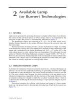
on salting out coefficients (h values) as they reported on. In Figure 5.3, values of He
obtained from
26
and
31
are plotted against pH at different temperature for comparative
reasons.
Finally, the work of Rischbieter et al.
17
considered the model of Weisember and
Schumpe
16
to determine the ozone solubility in aqueous solutions of different salts.
From data on ozone solubility in the absence and presence of salts, these authors
determined the h parameter values specific to ozone that were found to be as
follows
17
: h
G,0
= 3.96 × 10
–3
m
3
kmol
–1

and h
T
= 1.79 × 10
–3
m
3
kmol
–1
K
–1
for a
temperature range between 5 and 25ºC (see also Table 5.2 and Table 5.3).
He C
T
OH
=× −




−
384 10
2428
70035
. exp
.
Ha
kD C
k
n

OO
n
L
=
()
−
33
1
*
©2004 CRC Press LLC
5.2 KINETIC REGIMES OF THE OZONE
DECOMPOSITION REACTION
The rate of ozone decomposition can be catalogued as a pseudo first-order irreversible
reaction. This reaction is, in fact, a nonelementary one constituted by a mechanism
of steps that involve free radicals as explained in Chapter 2. When ozone is absorbed
in organic-free water, the system is also a gas–liquid reaction that develops in a
given kinetic regime. Knowledge of the kinetic regime of this reaction would aid to
conclude whether or not the decomposition reaction competes with any other direct
ozone reaction for the available ozone (i.e., when a compound B is also present in
water). Therefore, in this section, experimental conditions of the different kinetic
regimes for the ozone decomposition reaction to be hold are established.
Once the kinetic regime is known from the corresponding Hatta number, Ha
1
,
the reaction zone (the film or bulk water, see Figures 4.6 to 4.12) can be defined.
In this way, a comparison between the importance of the ozone decomposition and
ozone direct reactions with any compound B if also present in water can be made.
With this comparison it can be known through which type of reactions ozone acts
in water — through direct or indirect reactions.
The Hatta number or the reaction and diffusion times constitute the key parameter

to know. Then, the rate constant, individual liquid phase mass-transfer coefficient,
and ozone diffusivity are needed [see Equation (4.20)]. As will be shown later, the
kinetic regime will be highly dependent on the pH value. Then, the ozone decom-
position at three pH values (2, 7, and 12) will be treated here.
Application of Equation (4.19), on the other hand, leads to the ozone concen-
tration profile through the film layer. From experiments of ozone decomposition in
water carried out at pH 2 and 7, the rate constant of the ozone decomposition reaction
FIGURE 5.3 Variation of the Henry constant for the ozone–water system with pH and
temperature. (Continuous lines from Roth, J.A. and Sullivan, D.E., Solubility of ozone in
water, Ind. Eng. Chem. Fundam., 20, 137–140, 1981. With permission. Dotted lines from
Sotelo, J.L. et al., Henry’s law constant for the ozone–water system, Water Res., 23, 1239–1246,
1989. With permission.)
pH
He, kPa M
–1
2000
4000
6000
8000
10000
12000
2 4 6 8
T=20°C
T=12°C
T=5°C
©2004 CRC Press LLC
was found to be 8.3 × 10
–5
sec
–1

and 4.8 × 10
–4
sec
–1
, respectively.
34
For a higher
pH, let us say 12, a value of 2.1 sec
–1
can be taken as reported by Staehelin and
Hoigné
35
and Forni et al.
36
for the direct reaction between ozone and the hydroxyl
ion in organic free water. When the diffusivity of ozone is taken as 1.3 × 10
–3
m
2
/sec
(see 5.1.1), for two values of the liquid phase mass-transfer coefficient of 2 × 10
–5
m/sec
and 2 × 10
–4
m/sec, and Equation (4.19), Beltrán
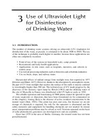
34
deduced the ozone concentration
profile through the film layer corresponding to these two situations at the three pH
studied. Figure 5.4 shows, as example, the results for the case of low mass transfer

(k
L
= 2 × 10
–5
m/sec).
On the other hand, Table 5.4 presents the values of Ha
1
. As can be seen, for pH
2 and 7, the kinetic regime corresponds to a slow reaction and, hence, the concen-
tration profile of ozone is nearly uniform through the film layer. In this case, the
reaction takes place completely in the bulk water. Notice that this is in agreement
with the kinetic treatment applied in Section 5.1.2 to determine the ozone solubility
and the Henry constant. For pH 12, on the contrary, the reaction has passed to a
moderate kinetic regime and then there is no available ozone in the bulk water. Here,
the reaction takes place in high extent in the film layer. The treatment applied in
Section 5.1.2 does not hold at pH 12.
On the other hand, Beltrán
34
also determined the reaction and diffusion times for
the ozone decomposition reaction from data on rate constant at different pH values and
the mass-transfer coefficients given above. In Figure 5.5 the reaction time of the ozone
decomposition has been plotted against pH showing the zones where the kinetic regime
is slow or fast. From Figure 5.5 it is deduced that at pH lower than 12, the ozone
decomposition reaction will not compete with the direct ozone reactions of fast or
FIGURE 5.4 Variation of the concentration of ozone with the depth of liquid penetration
during its absorption in organic-free water at steady state. Conditions: T = 20ºC, D
O3
= 1.3
× 10
–9

m
2
sec
–1
, k
L
= 2 × 10
–5
msec
–1
. (From Beltrán, F.J., Theoretical Aspects of the kinetics
of competitive ozone reactions in water, Ozone Sci. Eng. 17, 163–181, 1995. Copyright 1995
International Ozone Association. With permission.)
Gas–water
interface
Film layer
Bulk water
pH 2
pH 7
pH 12
C
O3b
=9.96 × 10
–6
M
C
O3b
=9.77 × 10
–6
M

C
O3b
=2.23 × 10
–6
M
C
O3
× 10
6
,

M
0
2
4
6
8
10
12
0 0.2 0.4 0.6 0.8 1
x
/δ
L
©2004 CRC Press LLC
instantaneous kinetic regime. On the contrary, at pH higher than 12, the ozone decom-
position reaction will be the only way of ozone disappearance when the ozone direct
reactions of compounds present in water, if any, develop in the slow kinetic regime. In
other words, depending on the kinetic regimes of the ozone decomposition and ozone-
B direct reactions, one of these reactions will be the only way to remove B from water
(the ozone decomposition because of the free radicals that would generate). This is of

significant importance since the absorption rate law, N
O3
, will take a different equation
(see Chapter 4). In Chapter 7 a more detailed comparison between the competition of
the ozone decomposition reaction and the direct ozone reactions is given.
TABLE 5.4
Hatta Values of the First-Order Ozone
Decomposition Reaction
a
pH k
L
= 2 ؋ 10
–5
msec
–1
k
L
= 2 ؋ 10
–4
msec
–1
20.016 0.0016
70.039 0.0039
12 2.57 0.257
a
Calculated from Equation (5.30) with n = 1 and k at 20ºC.
Source: From Beltrán, F.J., Theoretical Aspects of the
kinetics of competitive ozone reactions in water, Ozone Sci.
Eng. 17, 163–181, 1995. With permission.
FIGURE 5.5 Reaction time evolution of the ozone decomposition reaction with pH at 20ºC.

(From Beltrán, F.J., Theoretical Aspects of the kinetics of competitive ozone reactions in
water, Ozone Sci. Eng. 17, 163–181, 1995. Copyright 1995 International Ozone Association.
With permission.)
0 2 4 6 8 10 12 14
pH
Fast reaction zone
Slow reaction zone
t
R
, s
t
D
, =3.2 s
t
D
, =0.32 s
10
–4
10
–3
10
–2
10
–1
10
1
10
2
10
3

10
4
10
5
1
©2004 CRC Press LLC
5.3 KINETIC REGIMES OF DIRECT
OZONATION REACTIONS
A series of steps should first be done before starting with the kinetic study of direct
ozone reactions. Absorption rate equations for irreversible second order reactions
are not valid when ozone reacts in water not only with the target compound B but
also with intermediates formed from the first ozone-compound B direct reaction.
For this case, the more complex rate equations for series parallel reactions hold.
Therefore, in the kinetic study of single direct ozonation reactions, appropriate
experimental conditions should first be established for the ozone-B reaction to be
the only one consuming ozone. The competitive effect of the ozone decomposition
reaction can be eliminated by considering the kinetic regimes of this reaction and
the rate constant of the direct reaction under study (see Section 5.2). At pH lower
than 12, if both reactions (ozone decomposition and direct reaction) develop in the
same kinetic regime, the former reaction can be stopped by the addition of scavengers
of hydroxyl radicals. For example, Figure 5.6 shows, as example, the evolution of
the concentration of atrazine with time during ozonation experiments in water in
the presence and absence of tert-butanol or carbonate, known scavengers or inhibitors
of the ozone decomposition.
37
As can be seen, the presence of these substances slows
down the ozonation rate because they trap hydroxyl radicals and avoid the decom-
position of ozone (see ozone mechanism in Chapter 2).
FIGURE 5.6 Effect of hydroxyl radical scavengers on the ozonation of atrazine in water.
Conditions: C

ATZ0
= 5 × 10
–5
M, P
O3i
= 1050 Pa, With scavengers: pH: ∆=2, 0.05 M t-butanol,
▫=7, 0.075 M bicarbonate, ⅙=12, 0.075 M bicarbonate. Without scavengers: ᭡=pH 2, Ⅲ=pH 7,
●=pH 12. (From Beltrán, F.J., García-Araya, J.F., and Benito, A., Advanced oxidation of
atrazine in water. I. Ozonation, Water Res., 28, 2153–2164, 1994. Copyright 1994 Elsevier
Press. Reprinted with permission.)
0 5 10 15 20 25 30
C
B
/C
B
o
Time, min
0
0.2
0.4
0.6
0.8
1
©2004 CRC Press LLC
5.3.1 CHECKING SECONDARY REACTIONS
Once the ozone decomposition reaction has been suppressed, the next step before
accomplishing the kinetic study of any ozone-B direct reaction is to check the
importance of ozone reactions with intermediates. Importance of secondary reactions
can be established by calculating the global stoichiometric ratio at different times
as was shown in Section 3.2.1.

In some cases, the effect of secondary reactions is eliminated by reducing the
mass-transfer rate of ozone. For example, Beltrán et al.
38
carried out the ozonation
of some crotonic acid derived compounds in an agitated cell and in an agitated tank
(see Figure 5.7). The authors observed that the global stoichiometric ratio remained
constant (around unity) only when the reactions were carried out in the agitated cell.
Thus, in this reactor the ozone–acid reaction was the only one developing at the
conditions investigated. Hence, the agitated cell was the recommended reactor to
carry out the kinetic study for rate constant determination.
5.3.2 SOME COMMON FEATURES OF THE KINETIC STUDIES
Other aspects should be considered for the kinetic study of a gas–liquid reaction as
ozonation is. The first one is the establishment of the kinetic regime of ozone
absorption due to the fact that the absorption rate law equation varies depending on
the kinetic regime. For some kinetic regime, the absorption rate law is a simple
equation that contains the unknown parameter, mainly the rate constant, but for some
others the absorption rate law is a complicated equation that will be difficult to deal
with (see Chapter 4). Therefore, the appropriate kinetic regime should be not only
that with the absorption rate law containing the parameter to look for but also that
with the simpler mathematical equation, if possible. In this sense, Table 5.5 gives
the appropriate kinetic regime that allows the determination of parameters like the
reaction rate constant, volumetric mass-transfer coefficient, etc., together with the
corresponding absorption rate equations and conditions to be held. The kinetic
regime, as has been shown before, depends on the relative importance of chemical
and mass-transfer rate steps. This relationship can be established by calculating the
dimensionless numbers of Hatta (Ha
2
) and the instantaneous reaction factor (E
i
), the

latter needed only when the reactions are fast or instantaneous. However, a priori,
the Hatta number is also unknown since parameters such as the reaction rate constant
have to be determined [see Equation (4.40) for Ha
2
definition]. Thus, the kinetic
study should start from the assumption that at the experimental conditions to be
applied the kinetic regime is known and, then, the absorption rate law, N
A
(in
FIGURE 5.7 Experimental agitated cell for kinetic gas–liquid reaction absorption studies.
Ozonized gas
Nonabsorbed gas
©2004 CRC Press LLC
this case, N
O3
) (see Chapter 4). This means that some condition referring to the Hatta
number has to be confirmed (see also Table 5.5) once the rate constant and/or
individual liquid phase mass-transfer coefficient are known. In order to ensure that
the hypothesis is solid, some preliminary experiments can be done to classify the
kinetic regime as fast or slow. In these experiments, the concentration of dissolved
ozone is the key parameter to follow. Thus, the absence of dissolved ozone is a
definitive proof of fast or instantaneous regime while the opposite situation indicates
the kinetic regime is slow.
Interpretation of experimental results to study the direct ozonation kinetics is
accomplished with the use of ozone and B mass balance equations. The absorption
rate law, N
O3
, is one of the terms of these equations. The mathematical form of the
mass balance equation depends on the reactor type or, to be more exact, it depends
on the type of flow the gas and water phases present through the reactor used. Thus,

the second aspect to consider while studying the kinetics of ozonation reactions
concerns the type of reactor used for the ozonation experiments. For kinetic studies
at the laboratory, experiments are usually carried out in ideal reactors or reactors
with ideal flow for water and gas phases (see Appendix A1). Ideal reactors are those
that the application of some hypothesis allows the establishment of the mathematical
expression of the design equation, that is, the mass balance equation of any com-
pound present. In this way, a mathematical expression is readily available to fit the
experimental results and determine the kinetic parameters (rate constants, mass-
transfer coefficients, etc.).
For a continuous agitated tank (see Figure 5.1) where both the water and gas
phase are perfectly mixed and fed continuously to the reactor, the mass balance
equation for, let us say, the compound B in the ozone-B system, would be:
TABLE 5.5
Absorption Rate Law Equations for Different Kinetic Regimes of Ozonations
a
Kinetic
Regime Kinetic Equation
Conditions and Parameter
to Detemine
Very slow

Ha
2
< 0.02, C
O3
≠ 0
Rate constant
Diffusional

0.02 < Ha

2
< 0.3, C
O3
= 0
Mass-transfer coefficient
Fast Ha
2
> 3, C
O3
= 0
Rate constant or mass-transfer coefficients
Fast pseudo
first-order
3 < Ha
2
< E
i
/2, C
O3
= 0
Rate constant or specific interfacial area
Instantaneous Ha
2
> nE
i
, C
O3
= 0
Mass-transfer coefficient
a

Equations according to film theory. For stoichiometry, see Reaction (4.32) with A = Ozone. N
O
3
, ozone
absorption rate, Msec
–1
, Ha
2
according to Equation (4.40). E
i
, according to Equation (4.46), n = function
(Ha, E
i
). a represents the specific interfacial area.
NkaCC
dC
dt
r
OLOO
O
i
i
3
33
3
=−
()
=+
∑
*

NkaC
OLO
3
3
=
*
Nka
Ha
tahnHa
OL
3
2
2
=
NaCkDC
OODOM
3
33
=
*
NkaCE
OLOi
3
3
=
*
©2004 CRC Press LLC
(5.31)
where v
0

and V are the liquid volumetric flow rate and total reaction volume,
respectively, and β the liquid hold-up or fraction of liquid in the total volume.
Equation (5.31) would reduce to Equation (3.8) when the reactor is semicontinuous,
that is, when an aqueous solution of B is initially charged to the reactor.
If the gas phase being fed to the ozonation reactor is considered and perfect
mixing is also assumed, the ozone mass balance equation for the gas phase will be:
(5.32)
where v
g
is the volumetric gas flow of the gas phase, C
geb
and C
gb
the concentrations
of ozone in the bulk gas at the reactor inlet and outlet, respectively, and G′
O3
takes
a different form depending on the kinetic regime of absorption:
•For slow kinetic regime:
(5.33)
•For fast and instantaneous regime:
(5.34)
(where E is E
i
if the kinetic regime is instantaneous).
The perfect mixing is usually associated with the liquid and gas phases in
mechanically agitated tanks and, also, in some cases, with bubble reactors (see Figure
5.1). In this latter device, however, the plug flow is more common for the gas phase
flow. Plug flow, on the other hand, is associated with tubular reactors, such as the
bubble column. In this case, the concentration of reactants varies along the axial

length of the tube with no mixing at all. The ozone mass balance in the gas phase
is (see Appendix A1):
(5.35)
In practical situations or even at laboratory scale, the hypothesis for ideal flows
does not hold or the ideal reactor design equations. In these cases, a study of the
nonideal flow should be carried out. This study (see Appendix A3) leads to the
determination of the residence time distribution function (RTD) and allows the
reactor be modeled as a combination of ideal reactors or as an ideal reactor with
some sort of deviation from ideality.
39
In this way, the reactor design equations that
hold correspond to those of the ideal reactors that simulate the flow behavior in the
vC C rV V
dC
dt
B
Bb
B
Bb
00
−
()
+=ββ
vC C VG V
dC
dt
Acc
g
geb gb
O

gb
−
()
+
′
=− =ββ
3
1()
′
=−GkaCC
OLO
Ob
33
3
()
*
′
=GkaCE
OLO33
*
v
dC
dz
GS S
dC
dt
g
gb
O
gb

−
′
=−
3
1ββ()
©2004 CRC Press LLC
real reactor. Also, the RTD function can confirm that the flow through the reactor
presents ideal behavior. Some of these models will be discussed in Chapter 11 on
kinetic modeling of ozonation processes.
In the next sections, the ozonation kinetic study is carried out by considering
the following points:
• It will refer to one gas–liquid irreversible second order reaction between
ozone and one compound B present in water with no competition due to
secondary direct reactions unless indicated.
• There is no competition of indirect reactions.
•A given kinetic regime will be assumed that, in most cases, will be
confirmed once the kinetic parameters have been calculated.
•Unless indicated, the design equations will correspond to a bubble column
or mechanically-agitated bubble tank where a known volume of the water
phase containing compound B is initially charged. Ozone gas is then fed
continuously as an oxygen–ozone mixture of known concentration and
flow rate. Perfect mixing of both phases, water and gas, will be considered
unless indicated. The reactors are then semibatch ozonation contactors.
• Film theory will be applied unless indicated.
• The kinetic treatment will go from the instantaneous to the very slow
kinetic regime cases.
Table 5.5 shows the parameters usually determined when applied the kinetic
equations of the different kinetic regimes.
Some other common features of the kinetic study refer to the use of the ozone
solubility and mass-transfer coefficients.

5.3.2.1 The Ozone Solubility
In all absorption rate equation the ozone solubility term, C
O3
*, is present (see Table
5.5). This is also the ozone concentration at the gas–water interface (because equi-
librium conditions are assumed to hold instantaneously at the interface). Notice that
this concentration corresponds to that of ozone at gas–water interface in equilibrium
with the gas leaving the reactor because of perfect mixing conditions (see Appendix I).
Then, application of Henry’s law leads to
(5.36)
where P
O3s
is the ozone partial pressure in the gas at the reactor outlet. Since P
O3s
changes with time, it is more convenient to express C
O3
*
as a function of the ozone
partial pressure at the reactor inlet, P
O3i
, which stays constant and known. This can
be made with the use of the ozone mass balance in the gas phase, which is also
perfectly mixed [see Equation (5.32)]. Ozone partial pressures are expressed as a
function of concentrations with the gas perfect law:
(5.37)
PHeC
Os O33
=
*
PCRT

Os g3
=
©2004 CRC Press LLC
In many cases, the accumulation rate term in Equation (5.32) can be considered
negligible so that the ozone concentration in the gas at the reactor outlet becomes
(5.38)
then combination of Equations (5.36) to (5.38) allows C
O3
*
be expressed as a function
of C
geb
.
5.3.2.2 The Individual Liquid Phase Mass-Transfer Coefficient, k
L
The individual liquid phase mass-transfer coefficient, k
L
, is a key parameter to know
in order to determine the Hatta number (Ha
2
). Although this mass-transfer coefficient
can also be determined from chemical methods (see Section 5.3.3), some empirical
equations can be used. These equations mainly applied to very dilute solutions as
in most ozonation reactions in drinking water where the aqueous solution contains
low concentrations of B. For wastewater ozonation some deviations are found spe-
cially related to the specific interfacial area that affects the volumetric mass-transfer
coefficient, k
L
a as shown in Chapter 6.
For mechanically stirred reactors the following equation proposed by Van Dier-

endonck can be used
40
:
(5.39)
where SI units are used and Sc the Scmidth number is defined as:
(5.40)
with µ
L
and ρ
L
being the viscosity and density of the solution (water in this case).
In the case of bubble columns, Calderbank
40
also proposed Equation (5.39) for
bubble diameters, d
b
, higher than 2 mm and Equation (5.41) for d
b
< 2 mm:
k
L
= k
L

(for 2 mm)
500 db (5.41)
where the bubble diameter can be calculated from Equation (5.42):
(5.42)
where σ
L

and u
g
are the surface tension of the liquid (water in this case) and the
superficial gas velocity, respectively, and the fraction of gas phase, 1-β, can be
calculated from the equation
CC
VG
v
gge
O
g
=+
′
β
3
k
g
Sc
L
L
L
=
−
042
3
05
.
.
µ
ρ

Sc
D
L
LA
=
µ
ρ
61
2
05
025
()
.
.
−
=












β
ρ

σ
σ
ρ
d
g
u
g
b
L
L
g
L
L
©2004 CRC Press LLC
(5.43)
or simply from experimental data of the height the liquid has in the column, with
and without the gas being fed, h
T
and h, respectively:
(5.44)
Values of k
L
vary between 10
–5
and 10
–4
msec
–1
for laboratory bubble columns and
mechanically stirred reactors. In practice, the range of values is also similar, between

3 × 10
–5
and 2 × 10
–4
msec
–1
.
41
5.3.3 INSTANTANEOUS KINETIC REGIME
In the instantaneous kinetic regime the process rate is exclusively controlled by the
diffusion rate of reactants, ozone and B, through the liquid film closed to the
gas–water interface. For this kinetic regime the reaction develops in a plane inside
the film layer (see Figure 4.12 for concentration profiles through the film layer).
According to the film theory, the diffusion rates of ozone and B are the same, once
the stoichiometric ratio is accounted for:
(5.45)
Equation (5.45) allows x
R
, the distance to the interface where the reaction plane is
found (see Figure 4.12), be calculated. Also, x
R
is related to the reaction factor with
Equation (5.46):
(5.46)
The absorption rate law is given by Equations (4.45) and (4.46) that applied to the
ozone-B reaction become as follows:
(5.47)
with C
O3
*

calculated from Equations (5.36) to (5.38). Equation (5.47) holds if Ha
2
>
10E
i
(see also Table 5.5). Reactions of ozone with phenols at alkaline conditions
112
025
025
05
−=



























β
µ
σ
σ
ρ
.
.
.
.
uu
g
gL
L
g
L
L
1−=
−
β
hh
h
T
T

z
D
x
C
D
x
C
O
R
O
B
LR
Bb
3
3
*
=
−δ
x
D
kE
R
O
L
=
3
NkCEkC
DC
zD C
OLOiLO

B
Bb
OO
33 3
33
1==+






**
*
©2004 CRC Press LLC
(i.e., at pH > pK of the phenol) or reactions of ozone with some dyes are catalogued
as instantaneous reactions.
42,43
These reactions present very high rate constant values
that make the kinetic regime instantaneous. In this case, the condition of the instan-
taneous regime can first be checked to establish the experimental conditions to apply,
that is, the ozone concentration in the gas, B concentration, etc.
If the stoichiometric ratio, z, is accounted for, the absorption rate law also
expresses the chemical disappearance rate of the compound B. Then, the mass
balance of B in water in a semibatch well-agitated reactor becomes:
(5.48)
Integration of Equation (5.48) taking into account Equations (5.47) and (5.36) to
(5.38), finally yields
(5.49)
where

(5.50)
According to this method, a plot on the left side of Equation (5.49) against time
should lead to a straight line. From the slope of this line the volumetric mass-transfer
coefficient k
L
a is obtained. This procedure was used in a previous work
42
where the
ozonation of p-nitrophenol was studied. As example, Figure 5.8 shows the plot
mentioned prepared from experimental data of the ozonation of p-nitrophenol at
pH 8.5. The instantaneous kinetic regime is confirmed from the values of Ha
2
and
E
i
. Given the fact that the rate constant of this reaction is about 14 × 10
6
M
–1
sec
–1 42
the Hatta number resulted to be much higher than E
i
and condition of instantaneous
regime is fulfilled. This procedure has also been applied in other works, where the
ozonation of resorcinol, phloroglucinol and 1,3 cyclohexanedione, considered pre-
cursors of trihalomethane compounds in water, was studied.
44,45
In these cases,
however, the value of k

L
a obtained can be taken as a lower limit for this coefficient.
This is so because C
O3
*
was directly calculated by application of the Henry’s law to
the gas at the reactor inlet and not from Equations (5.36) to (5.38), a situation that
does not exactly correspond to the perfect mixing conditions of the water phase.
Then, values of C
O3
*
used in their calculations were higher than the correct ones that
should be obtained from the ozone partial pressure at the reactor outlet as indicated
above. In any case, the k
L
a values were in the range expected for this type of
parameter.
41
−=
dC
dt
zN a
Bb
O3
ln ϑ=−
kaD
D
t
LB
O3

ϑ=
+
+
C
zD C
D
C
zD C
D
Bb
OO
B
Bo
OO
B
33
33
*
*
©2004 CRC Press LLC
A more rigorous treatment, however, was made by Ridgway et al.
43
that also
determined the volumetric mass-transfer coefficient of a gas–liquid reactor from the
results of an instantaneous reaction. In this case, the reaction used was between
ozone and the blue dye: indigo disulfonate of potassium. These authors
43
used the
Danckwerts theory for instantaneous reactions, that is, Equation (4.68) instead of
Equation (4.46) to calculate E

i
. They did no neglect the influence of the accumulation
rate term, Acc, in Equation (5.32). From Equations (4.68), (5.32), (5.36), and (5.37)
they arrived to the following equation for the absorption rate law:
(5.51)
where
(5.52)
Then, they introduced the molar balance of B [Equation (5.48)] and, finally, inte-
grated the resulting equation to yield
43
:
(5.53)
FIGURE 5.8 Determination of the volumetric mass-transfer coefficient from ozonation exper-
iments of p-nitrophenol in the instantaneous kinetic regime at pH 8.5. (From Beltrán, F.J.,
Gómez-Serrano, V., and Durán, A., Degradation Kinetics Of p-Nitrophenol Ozonation in Water,
Wat. Res., 26, 9–17, 1992. Copyright 1992 Elsevier Press Reprinted. With permission.)
Ozonation time, min
0 5 10 15 20
ln ϕ
0
0.5
1
1.5
2
Na
C
zCD
D
z AccD
vD

z
ka
D
D
VD
vD
O
Bb
ge O
B
O
gB
l
O
B
O
gB
3
3
3
33
=
+−
+
α
α
αβ
α=
He
RT

ln
*
C
zCD
D
z AccD
vD
C
zD C
D
z AccD
vD
ka
D
D
VD
vD
t
Bb
ge O
B
O
gB
Bo
OO
B
O
gB
L
O

B
O
gB
+−
+−














=−
+
α
α
α
αβ
3
3
33 3
33
1

1
©2004 CRC Press LLC
From the slope of a plot similar to that used in Figure 5.8, k
L
a

is obtained. Notice
now that the method requires the application of a trial and error procedure because
the accumulation rate term is unknown. The experiments were carried out at pH 4
and the instantaneous criteria was confirmed (the rate constant for the reaction was
about 10
9
M
–1
sec
–1
). Table 5.6 gives experimental conditions and values of k
L
a
calculated in these works.
5.3.4 FAST KINETIC REGIME
For the fast kinetic regime the reaction develops in a zone close to the gas–water
interface (see Figures 4.10 and 4.11). By comparison to the instantaneous regime,
here, the reaction is in a zone in the film layer. The condition for this kinetic regime
is that Ha
2
> 3 (see Table 5.5). The general equation for the absorption rate law is
given by Equation (4.44). This equation, however, gives results difficult to handle
for kinetic determination. A possible simplification comes from the possibility that
the concentration profile of B through the film layer should be constant and the same

as in the bulk concentration C
B
= C
Bb
(see Figure 4.11). If this case holds, it is said
that the kinetic regime is fast of pseudo first-order. For an ozonation reaction of this
type, Ha
1
= Ha
2
with k
1
= k
2
C
Bb
. The absorption rate law simplifies to Equation (4.48)
that in the case of ozone becomes
(5.54)
As can be observed, the reaction rate constant, k
2
, is present in Equation (5.54) that
results in a simpler mathematical use for its determination.
The procedure to follow for the rate constant determination is similar to that
presented above for the volumetric mass-transfer coefficient when the reaction is
instantaneous. The first step is the assumption that the fast of pseudo first-order
kinetic regime holds at the experimental conditions applied. Then, the molar balance
of B is introduced for a batch system and related to the ozone absorption rate for
this kinetic regime with the use of Equation (5.48). Then, Equation (5.55) is obtained:
(5.55)

Integration of Equation (5.55) between the limits:
(5.56)
leads to the calculation of k
2
. Finally, condition (4.47) has to be checked. This
procedure has been applied in some works with some approximations. Thus, Sotelo
et al.
44,56
determined the rate constants of the reaction between ozone and resorcinol,
phloroglucinol, and 1,3 cyclohexanedione by assuming this kinetic regime holds at
Na aC kCD
OO
Bb
O3323
=
*
−=
dC
dt
zaC k C D
Bb
O
Bb
O32 3
*
tCC
ttC C
Bb Bb
Bb Bb
==

==
0
0
©2004 CRC Press LLC
TABLE 5.6
Works on Heterogeneous Direct Ozonation Kinetics
Compound Observations
Reference #
and Year
Phenol Wetted wall column, S = 160 m
2
, 15ºC, pH: 1.75–12,
Moderate kinetic regime with Ha = 1, different reaction
controlling step according to pH. At alkaline conditions,
n = 0, m = 1. k
L
= 6.7 × 10
–5
(pH 3 and 4), k = 1.8 × 10
9

(O
3
-Phenolate)
46
(1978)
Phenol Wetted wall column, S = 160 m
2
, 9, 15 and 20ºC, pH not
given; Moderate kinetic regime with Ha = 1, AE =

14200 calmol
–1
47
(1978)
Pure water Semibatch agitated reactor, 12–25ºC, PMC, Slow kinetic
regime. Determination of k
L
a at different agitation speeds
48
(1980)
Dyes 500-ml washing bottles with plate diffuser, pH 7,
phosphate buffer, 20–22ºC, 1/z between 1.7 (O
3
-Direct
Yellow 12) and 12 (O
3
-Acid Red 151). PMC,
instantaneous kinetic regime
49
(1983)
Phenols Semibatch reactor, PMC, pH 2.5–3, Fast pseudo first-order
kinetic regime, CK, determination of relative rate constants
50
(1984)
Maleic acid 0.75-L semibatch stirred bubble reactor, 20ºC, pH 2.53 and
2.69, PMC, GCM, moderate–diffusional kinetic regime,
k = 1930
51
Indigo disulfonate Semibatch standard agitated tank, Diam = 0.29 m., 25ºC,
pH < 4, PMC, instantaneous kinetic regime, Danckwerts

theory applied, k
L
a = 0.048 (8 rps)
43
(1989)
o-Cresol 0.75-L semibatch stirred bubble reactor, 20ºC, pH 2,
phosphate buffer, 1/z = 2 from homogeneous ozonation,
PMC, GCM, fast pseudo first-order kinetic regime, k =
11955
52
(1990)
Pure water and
resorcinol, and
phloroglucinol
0.75-L semibatch stirred bubble reactor, 1–20ºC, pH 2,7,8.5
phosphate buffer, PMC, GCM, Slow kinetic regime, k
L
a
varies depending on gas flow rate and agitation speed:
k
L
a = 3.69 × 10
–3
(pH 7, 20ºC, 700 rpm, 30 Lh
–1
). From
homogeneous and heterogeneous ozonation of phenols
studied: 1/z = 2 (O
3
-resorcinol), 1/z = 1.6

(O
3
-phloroglucinol). Some intermediates identified
53
2-hydroxypyridine 1-L semibatch stirred bubble reactor, 20ºC, pH 5, 20 mM
t-butanol, PMC, slow kinetic regime, three well mixed
reactor models, Determination of rate constant of ozone
reactions with parent compound and intermediates, and
mass-transfer coefficient through fitting experimental
results to mass balance equations
54
(1991)
Malathion 0.5-L semibatch stirred bubble reactor, 10–40ºC, pH 2–9,
1/z = 3 from homogeneous kinetics, PMC, GCM, slow
kinetic regime, n = m = 1, k = 98.8 (20ºC, pH 7), AE =
38.9 kJmol
–1
55
(1991)