Ozone Reaction Kinetics for Water and Wastewater Systems - Chapter 11 (end) ppt
Bạn đang xem bản rút gọn của tài liệu. Xem và tải ngay bản đầy đủ của tài liệu tại đây (2.54 MB, 73 trang )
©2004 CRC Press LLC
11
Kinetic Modeling of
Ozone Processes
The last step of a kinetic study is building a kinetic model in which all the information
obtained from some of the methods presented so far is applied. As in any system
that involves chemical reactions and mass transfer, the kinetic model for ozonation
processes is constituted by the mass balance equations of the species present (ozone,
reacting compounds, hydrogen peroxide, etc.) in the system, which is the reactor
volume. In addition, for the particular case of gas–liquid reacting systems, depending
on the kinetic regime of ozone absorption, the mathematical model can also include
microscopic mass balance equations applied to the film layer close to the gas–water
interface, which are needed to determine the mass flux of species to or from the
liquid or gas phases through the interface. In the first case (slow regime), the
mathematical model is usually a set of nonlinear ordinary or partial differential or
algebraic equations of different mathematical complexity. In the second case (fast
regime) the mathematical complexity is even higher since the solution implies trial-
and-error methods, together with numerical solution techniques for both the bulk
mass balance equations and microscopic differential equations.
1
In any case, solution
of this model will allow the concentrations of the different species to be known at
the reactor outlet or at any time, depending on the regime of ozonation (batch,
semibatch, or continuous).
The kinetic model is built up from the application of mass balances to an
increment volume of reaction,
∆
V, where the concentration of any species can be
considered uniform and constant in space. Thus, for a species
i
, the general mass
balance equation in an element of reactor,
∆
V, is:
(11.1)
where
F
i
0
and
F
i
represent the molar rates of species
i
, at the entrance and exit of
the reaction volume,
∆
V
, respectively;
G
i
, the generation rate that represents the
i
mole rate per unit of volume that is formed or removed;
∆
n
i
/
∆
t
the accumulation
rate of
i
in that volume; and
β
the liquid holdup or liquid fraction of reaction volume.
Since water ozonation systems do not involve variations of temperature, ozonation
can be considered an isothermic system, and an energy balance is not required.
The small volume considered,
∆
V
, is divided into liquid and gas fractions that
can be measured through the liquid holdup,
β
, defined in Equation (5.43) or Equation
(5.44). Also, volume variations in ozonation systems are negligible especially for
the water phase (density being constant). In the case of the gas phase, some variation
due to the drop in pressure should be taken into account, especially in real
FFGV
n
t
iii
i
0
−+ =β∆
∆
∆
©2004 CRC Press LLC
ozone contactors several meters high. For laboratory or pilot plant ozone reactors,
variation of total gas pressure can be neglected. According to this, for a system of
constant volume or constant volumetric flow rates through the ozone reactor, Equa-
tion (11.1) reduces to Equation (11.2) and Equation (11.3), for any gas or liquid
component, respectively.
For a gas component:
(11.2)
For a liquid component:
(11.3)
with
C
i
being the concentration of species i in this volume
(11.4)
where subindex
x
can be
L
or
g
to refer to the liquid or gas phase, respectively.
Consequently,
v
L
and
v
g
are the actual liquid and gas volumetric flow rates through
the reactor, respectively.
For the liquid phase:
(11.5)
and for the gas phase:
(11.6)
where
v
L
0
and
v
g
0
are the corresponding volumetric flow rates for the water and gas
phases at empty reactor conditions. For continuous systems, the volumetric flow
rates can also be expressed as a function of hydraulic residence times,
τ
, since:
(11.7)
The generation term in Equation (11.1) is a very important function that in gas–liquid
reaction systems such as ozonation presents different algebraic forms depending on
the kinetic regime of absorption and the nature of
i
species. Here also, one should
determine the balance equation in the gas or liquid phase as far as the form of the
generation rate term is concerned.
v
C
V
G
C
t
g
i
i
i
∆
∆
∆
∆()11−
+
−
=
β
β
β
v
C
V
G
C
t
L
i
i
i
∆
∆
∆
∆β
+=
C
F
v
i
i
x
=
vv
LL
=
0
β
vv
gg
=−
0
1()β
τ=
V
v
0
©2004 CRC Press LLC
The forms of the generation rate term in most common cases are as indicated
in the following sections.
11.1 CASE OF SLOW KINETIC REGIME
OF OZONE ABSORPTION
When reactions of ozone develop in the bulk water (see Chapter 5) the kinetic regime
is slow or the ozone reactions are slow. This is the typical kinetic regime of drinking
water ozonation systems. In these cases the generation rate term of Equation (11.1)
is as follows:
For the water phase:
1. For any nonvolatile species
i
:
(11.8)
where
r
i
is the reaction rate of
i
due to chemical reactions
(11.9)
where subindex
j
refers to any
j
reaction that species i undergoes in water.
For example, in an ozonation system,
r
i
of a given compound will involve
at least two reactions: the direct reaction with ozone and the free radical
reaction with the hydroxyl radical. For a general case where UV radiation
is also applied, another possible contribution is due to the direct photol-
ysis. Then, the reaction rate of the compound
i
is expressed as the sum
of the rates due to these three contributions:
(11.10)
Notice that these contributions, once substituted in Equation (11.2), have negative
signs because the stoichiometric coefficients of their corresponding reactions are
negative (see Section 3.1). Also, the exact form of Equation (11.10) will depend on
the expression for the concentration of hydroxyl radicals which is usually defined
as in Equation (7.12), Equation (8.5), or Equation (9.39).
2. For any volatile species
i
:
(11.11)
where
N
vi
represents the desorption rate of i. Here,
C
i
* is the concentra-
tion of i at the water interface that can be expressed as a function of the
Gr
ii
=
rr
iij
=
∑
rr r r
iDUV
Rad
=+ +
GN r kaCC r
iviiL
i
ii i
=+=
()
−
()
+
*
©2004 CRC Press LLC
partial pressure of
i
or the gas concentration of i,
C
gi
, with the corre-
sponding Henry’s law:
(11.12)
In this equation it is assumed that the gas phase resistance to mass transfer
is negligible.
3. For ozone in the water phase
(11.13)
where
r
O
3
is the reaction rate term that involves all the chemical reactions
ozone undergoes in water and
N
O
3
is the ozone transfer rate from the gas
to the water phase:
(11.14)
and
(11.15)
where
C
O
3
g
is the concentration of ozone in the gas phase. In ozonation
systems, Equation (11.15) always holds because the gas resistance to
ozone transfer is negligible (ozone is sparingly soluble in water
2
;
see also
Section 4.2.3). Also, the exact form of the reaction rate term,
r
O
3
, is
deduced from the mechanism of the reactions proposed. For example, the
concentration of ozone is a function of the concentration of hydroxyl
radicals that depends on the oxidizing system used, as observed in Chapter 7
to Chapter 9.
For the gas phase:
1. For any
i
volatile species:
(11.16)
2. For ozone:
(11.17)
where the minus sign means that ozone is being transferred from the gas
into the water phase.
PHeC CRT
iviigi
==
*
GN r
iOO
=+
33
NkaCC
OLOO333
=−
()
*
PHeCCRT
OOOg333
==
*
GN N kaCC
i vgi vi L
i
ii
==−=
()
−
()
*
GN N kaC C
iOg g LO O
==−=− −
()
333
*
©2004 CRC Press LLC
11.2 CASE OF FAST KINETIC REGIME
OF OZONE ABSORPTION
This is a rather unusual case in drinking water treatment because the fast kinetic
regime mainly predominates when the concentration of compounds that react with
ozone in water are high enough so that the Hatta number of ozone reactions goes
higher than 3 (see Table 5.5). Another possibility of the Hatta number being higher
than 3 arises when the rate constants of the reactions of ozone and compounds
present in water are also very high, although the usual case is the former one. As a
consequence, the fast kinetic regime mainly develops in the ozonation of wastewater
as presented in Chapter 6 and in a few other specific cases. In the following text a
few examples of the absence or presence of the fast regime are given. Thus, let us
assume that the water contains some herbicide such as mecoprope. The direct rate
constant of the ozone–mecoprop reaction is 100 M
–1
s
–1
.
3
For to the fast kinetic regime
condition to be applied (see Table 5.5), the concentration of mecoprop in water
should be higher than 0.8
M
. This is an unrealistic value for the concentration of
herbicide because the kinetic regime in an actual case would likely be slower and
values of
G
i
would correspond to equations in Section 11.1 above. However, if the
compound present in water is a phenol (present, for example, in wastewaters), the
situation could change because the ozone–phenol reaction rate constant, let us say
at pH 7, would be about 2
×
10
6
M
–1
s
–1
. In this case, the kinetic regime would be
fast if the concentration of phenol is at least 5
×
10
–5
M
, which is a possible situation.
Another possible case of fast regime arises also when a phenol compound is treated
at high pH. Because of the dissociating character of phenols, the increase in pH
leads to increase in the concentration of the phenolate species which reacts with
ozone faster than the nondissociating phenol species (see Chapter 2). Then, an
increase in the rate constant yields an increase in the Hatta number and the conditions
for fast regime holds. For example, the literature reports studies about the kinetic
modeling of certain chlorophenol compounds in alkaline conditions where the fast
kinetic regime holds.
4–7
However, these cases are more likely specific to wastewater
where the concentration can be followed with the COD that will simplify the
mathematical model as will be shown later (see also Chapter 6).
Generally, when the kinetic regime is fast, the parameter difficult
G
i
is difficult
to determine, except in the case of ozone, when it undergoes a simple irreversible
reaction. In fact,
G
O
3
(in absolute value) has the same expression for the gas and
water phases:
(11.18)
where
E
, the reaction factor, depends on the fast kinetic regime type (moderate, fast,
of pseudo first order, instantaneous, etc.) to take one of the forms presented in
Chapter 4. However,
N
O
3
can only be used in the Equation (11.1) for ozone in the
gas phase. In the water phase, Equation (11.1) for ozone is not used since the
concentration of ozone,
C
O
3
, is zero when the kinetic regime is fast.
A different situation is presented when Equation (11.1) is applied to any other
species reacting with ozone. For such species, the generation term,
G
i
, as indicated
in Equation (11.8) or Equation (11.11), will depend on their concentrations
GN kaCE
iOLO
==
33
*
©2004 CRC Press LLC
(including that of ozone). But if C
O3
is zero, how can this situation be dealt with?
In the fast kinetic regime, the concentration of ozone is not zero only within the
liquid film layer, as already shown in Figure 4.10 to Figure 4.12. In fact, the
concentration of ozone varies from C
O3
*
at the gas–water interface to zero at a
given point within the film layer (between interface and bulk water). Also, the
concentration of the reacting species changes within the film layer. In these cases,
the maximum value of C
i
is in bulk water. If concentrations are not constant
within the film layer, how can G
i
be calculated? There are a few possible ways
to solve this problem. All of these however, involve the solution of the microscopic
mass balance Equation (4.34) and Equation (4.35). One of these possibilities
follows the complicated steps shown below:
• Calculate the concentration profiles of reacting species, including that of
ozone, with the position in the film layer (depth of penetration). This
requires the solution of the microscopic mass balance equations of species
(Equation (4.13) or Equation (4.34) and Equation (4.35) if film theory is
applied) through numerical methods.
•Determine the generation rate terms from the mean values of the reaction
rate terms once the concentrations of reactants are known at different
positions within the film layer. This can be accomplished as follows:
(11.19)
where r
i
is given by Equation (11.10).
• Solve the system of macroscopic mass balance Equation (11.1) with the
known values of G
i
.
The second possibility is the determination of the mass flux of reacting species
and ozone gas through the edge of the liquid film layer in contact with the bulk
liquid and through the gas-film layer in contact with the bulk gas, N
ib
l
and N
O3b
g
,
respectively.
For any reacting species, i:
(11.20)
and for ozone gas:
(11.21)
Notice that in Equation (11.21) the flux of ozone through the gas-film layer is the
same as through the interface because of the absence of gas resistance to mass
Grdx
ii
=
∫
1
0
δ
δ
GN D
C
x
i
ib
l
i
i
x
==−
∂
∂
=δ
GN D
C
x
kC E
O
Ob
g
i
i
x
LO3
3
0
3
==−
∂
∂
=
=
*
©2004 CRC Press LLC
transfer.
1
As also seen in Equation (11.21), the ozone flux is finally expressed as a
function of the reaction factor, E. Values of E and bulk mass flux of compounds,
N
ib
l
, can be calculated from the solution of continuity Equation (4.13) or Equation
(4.34) and Equation (4.35) as the film theory is applied. For example, in the case
of an irreversible second order reaction between ozone and B [Reaction (4.32)],
values of E can be known from the equations deduced in Section 4.2.1.2. (see also
Table 5.5). E and the bulk mass flux of compounds through the liquid film layer–bulk
water are then used in the bulk mass balances of species Equation (11.2) and
Equation (11.3) applied to the whole reactor volume, see later] to obtain the con-
centration profiles with time or position, depending on the type of flow of the gas
and water phases through the reactor and the time regime (stationary or nonstation-
ary) of ozonation. For example, Hautaniemi et al.
4
used this approach to predict the
concentration profiles of some chlorophenol compounds and ozone, when ozonation
was carried out at basic conditions in a semibatch, perfectly mixed tank.
It is evident that the mathematical model results are very complex to solve,
especially for multiple series parallel ozone reactions, which would be the usual
case. Nonetheless, there is one possible case that could even lead to one analytical
solution, i.e., when ozone, while being absorbed in water, undergoes a unique
irreversible reaction with the compound B already present in water. This can either
be the typical case of wastewater ozonation where COD can represent the concen-
tration of the matter present in water that reacts with ozone [Reaction (6.5)], or just
the case of one irreversible reaction between ozone and a compound B with a high
rate constant (i.e., a phenol compound). Two methods can be applied depending on
the time regime conditions. In both cases, however, the only generation term needed
is that of ozone, G
O3
= N
O3
. At nonsteady state conditions the method needs the mass
balance of B in bulk water, and at steady state conditions a total balance is the
recommended option, so that the corresponding generation rate term of B or COD
is not needed in this second approach. In this chapter, the procedure based on the
total balance will be followed to present the different solutions except in some cases
where the use of the bulk mass balance of B is already applied (see Section 11.6.2.1.).
In Section 11.8, an example of the kinetic model for the ozonation of industrial
wastewater in the fast kinetic regime is presented. In Section 6.6.3.1, a kinetic study
to determine the rate coefficient of the reaction of ozone and wastewater of high
reactivity was presented.
11.3 CASE OF INTERMEDIATE OR MODERATE KINETIC
REGIME OF OZONE ABSORPTION
When reactions of ozone develop both in the film close to the gas–water interface
and in bulk water, the kinetic regime is called intermediate or moderate. In this case,
there is a need to quantify the fraction of ozone reactions in both zones of water.
The problem is similar to that presented for fast reaction in the preceding section
but it includes the difficulty of reaction in bulk water as well. Again, the solution to
the problem implies the simultaneous solution of microscopic equations in the film
layer and macroscopic equations in the bulk water. This complex problem has been
©2004 CRC Press LLC
recently treated by Debellefontaine and Benbelkacer
8
by introducing the concept of
the depletion factor, F, previously defined by Schlüter and Schulzke.
9
This dimen-
sionless number, in a way similar to as the reaction or enhancement factor, E,
compares the ozone absorption (in this case) at the edge of the film in contact with
bulk water (N
O3
)
x = l
with the physical absorption of ozone. Definition of the depletion
factor is:
(11.22)
Notice that the depletion factor is defined as the number of times the ozone physical
absorption rate is increased due to the presence of chemical reaction in the bulk
water, while the reaction factor is defined as the number of times the maximum
physical ozone absorption rate (k
L
C
O3
*
) is increased due to chemical reactions in the
film layer. If a moderate regime is considered, chemical reactions develop both in
the film and in the bulk water (see Figure 4.9) so that the bulk ozone concentration
is different from zero (C
O3
≠ 0), in most cases. Hence, in this situation, the reaction
factor can also be defined as follows:
(11.23)
It is evident, according to definitions of E and F, that the ratio between the two
dimensionless numbers (F/E) represents the fraction of unconverted ozone that
leaves the film, entering the bulk water. Thus, application of Equation (11.22) and
Equation (11.23) allows the generation rate terms of ozone and reacting species in
the bulk water and the film layer, respectively, to be know separately. These terms
are as follows:
For the generation rate of ozone (reacted) in the film:
(11.24)
For the generation rate term of ozone (reacted) in the bulk water:
(11.25)
In a similar manner, for any compound B, reacting with ozone, the generation rate
terms in both the film and bulk water will be similar to those of Equation (11.24)
and Equation (11.25) once the stoichiometric coefficients are accounted for. For
example, for a compound i that reacts with ozone according to the stoichiometry
given by Reaction (3.5), the generation rate terms would be:
F
N
kC C
D
dC
dx
kC C
O
x
LO O
O
O
x
LO O
=
−
()
=
−
−
()
==
3
33
3
3
33
λλ
**
E
N
kC C
D
dC
dx
kC C
O
x
LO O
O
O
x
LO O
=
−
()
=
−
−
()
==
3
0
33
3
3
0
33
**
GEFkaCC
O film
LO O
3
33
=− −
()
()
*
Gr
O bulk
O
3
3
=
©2004 CRC Press LLC
In the film layer
(11.26)
In the bulk water
(11.27)
With this approach, Debellefontaine and Benbelkacen prepared the kinetic model
of the ozonation of maleic and fumaric acids.
10,11
More details of the use of Equation
(11.24) to Equation (11.27) are given in Section 11.6.3.
11.4 TIME REGIMES IN OZONATION
Once the generation rate terms have been specified, Equation (11.1) and Equation
(11.2) can further be simplified according to the effect of time on the performance
of the system. Thus, although the gas phase is continuously fed to the ozone
contactor, the water phase could be initially charged (batch system) or continuously
fed (continuous system). Either way, the time regime is directly related to the size
of the ozone contactor that depends on the volume of treated water. Usually, in
laboratory contactors, a semibatch system (continuous for the gas phase and batch
for the water phase) is used to carry out the ozone reactions. In some pilot plant
contactors, both the semibatch and continuous systems are possible, while in actual
ozone contactors in water or wastewater treatment plants, the continuous system is
the way of operation. The time regime (batch or continuous) is, thus, an important
aspect in reactor design since Equation (11.1) can significantly be simplified depend-
ing on the time regime type. For example, in semibatch systems, for the water phase,
there is no mass flow rates at the inlet and outlet of the reaction volume, and F
i0
and F
i
are not present in Equation (11.1) which then becomes:
(11.28)
In fact, for the water phase, this is the equation that has been used for kinetic studies
(see Chapter 5). Laboratory ozonation systems are examples where these equations
are applied since they usually are nonstationary processes where concentrations in
water vary with time.
For continuous systems (some pilot plants and comercial contactors), although
convection flow rates, F
i0
and F
i
, cannot be removed from Equation (11.1), the
accumulation rate terms, ∆n
i
/∆t, are not present since these are steady state processes.
In a steady state process, Equation (11.1) reduces to:
(11.29)
G
z
EFkaC C
i film
i
LO O
−
=− −
()
[]
1
33
()
*
Gr
i bulk
i
−
=
G=
C
t
i
i
∆
∆
∆
∆
C
Gi
i
τ
+=0
©2004 CRC Press LLC
It is evident that, in a practical case, there will be a period of time at the start of the
process when ozonation is a nonsteady state operation and Equation (11.1) cannot
be simplified. This represents the most difficult case to treat mathematically. Simi-
larly, also for practical applications, ozone contactors are designed for the steady
state operation so that Equation (11.1) is solved starting from Equation (11.29). In
fact, solving Equation (11.1) without any simplification is a rather academic exercise,
although it allows the process time to reach the steady state operation.
11.5 INFLUENCE OF THE TYPE OF WATER AND GAS FLOWS
Once the time regime has been established (semibatch or continuous systems, sta-
tionary or nonstationary operation), Equation (11.1) or Equation (11.2) and Equation
(11.3) have to be applied to the whole reaction volume to proceed with their solution.
This requires the type of phase flow be known. There are two main ideal flows for
which Equation (11.1) can be expanded to the whole reaction volume. These are
the perfectly mixed flow (PMF) and the plug flow (PF), which are based on the
hypothesis given in Appendix A1. It is also necessary to remember that G
i
values
in Equation (11.1) can involve the solution of microscopic differential mass balance
Equation (4.34) and Equation (4.35) within the liquid-film layer, in cases where the
kinetic regime of ozonation is fast or moderate.
For the cases of PMF and PF, Equation (11.1) applies as follows:
• Perfectly mixed flow (PMF)
(11.30)
where C
i0
and C
i
refer to the concentrations of i at the reactor inlet and
outlet, respectively. The hydraulic residence time, τ, coincides with the
mean residence time obtained from the residence time distribution func-
tion (see Appendix A3).
Notice, however, that some authors consider the whole reactor volume divided
into three zones of perfect mixing conditions: the water phase with volume V
L
, the
bubble phase with volume V
B
, and the free board or space above the free surface of
water with volume V
F
.
12
Thus, in some kinetic modeling works, Equation (11.30) is
applied to yield a system with three mass balance equations
12,13
(see later) because
a different ozone concentration is assumed in each phase.
• Plug flow (PF)
In this case, Equation (11.31) applies:
(11.31)
1
0
τ
CCG
dC
dt
iii
i
−
()
+=
−
∂
∂
+=
∂
∂
C
G
C
t
i
i
i
τ
©2004 CRC Press LLC
This equation can be integrated from the start of the process, (t = 0) and for the
whole reaction volume (τ = 0 to τ = V/vo).
One important difference observed between Equation (11.30) and Equation
(11.31) is that when the systems are at the steady state, the model with PMF is a
set of algebraic nonlinear equations, while models with PF are constituted by a set
of first order partial differential equations.
In actual contactors (even of laboratory size), however, the type of gas and water
flows can deviate from the ideal cases. Hence, tracer studies have to be carried out
to determine the residence time distribution function, RTDF, as shown in Appendix
A3. The RTDF can allow the real flow to be simulated as a combination of ideal
flows or as another ideal flow model of specific characteristics. These are called
models for nonideal flow.
14
The most commonly applied nonideal flow models are
the N perfectly mixed tanks in series model and the axial dispersion model described
in Appendix A3. When the flow is simulated with N perfectly mixed tanks in series,
Equation (11.30) also applies but it has to be solved N times. This is so because the
concentration of any species at the outlet of the last N-th reactor would represent
the concentration of the treated species at the actual contactor outlet. The dispersion
model represents a more complicated picture because it assumes that the flow is due
to both convection and axial diffusion.
14
As a consequence, the mass flow rates
[F terms in Equation (11.1)] are not only due to the convection flow contribution
(volumetric flow rate times the concentration) but also to the axial diffusion transport
which is given by the Fick’s law:
(11.32)
where U represents the superficial velocity of the phase through the reactor. Then
the total flow rate, F, in this model is:
(11.33)
where D
i
is the axial dispersion coefficient of the i species in the phase.
For an element dV, the mass balance (11.1) is:
(11.34)
that it becomes Equation (11.35), once Equation (11.7) and Equation (11.33) have
been taken into account:
(11.35)
ND
U
C
ad
i
i
=−
∂
∂
1
τ
FvCSN vCD
S
U
C
ii
ad
ii
i
=+ =−
∂
∂
00
τ
−∂ + ∂ =
∂
∂
FG V
n
t
ii
i
β
−
∂
∂
+
∂
∂
+=
∂
∂
CD
U
C
G
C
t
iii
i
i
ττ
2
2
2
©2004 CRC Press LLC
or as a function of the contactor height, z:
(11.36)
Equation (11.36) has to be integrated from the start of the process (t = 0), and for
the whole reaction volume (τ = 0 to τ = V/vo or better for z = 0 to z = H), which
usually requires numerical methods.
15,16
In addition to the classical or ideal models described above, literature also reports
several more sophisticated models that represent modifications of the N perfectly
mixed tanks in series and axial dispersion models. For example, El-Din and Smith
17
proposed the nonisobaric steady state one-phase axial dispersion model (1P-ADM)
that is constituted by nonlinear second order ordinary differential equations repre-
senting the mass balance of species in the water phase. These equations are as those
in the axial dispersion model [Equation (11.35)] with the concentration of ozone in
the gas phase at any point in the column, z, which is present in the ozone mass
transfer rate term, G
i
, expressed as an exponential function of position:
(11.37)
where C
O3g0
is the concentration of ozone at the column entrance. Of course, coef-
ficient ζ is an empirical parameter that has to be determined experimentally. The
use of Equation (11.37) allows the omission of the ozone mass balance in the gas
phase. This model can be useful in the case of kinetic models of ozone absorption
and decomposition in water because balance equations for reacting compounds in
water are not needed. For detailed information on this model see Reference 17.
Another kinetic model reported in the literature that presents a modification of
the ideal N perfectly mixed tanks in series model is called the transient back flow
cell model (BFCM).
18
As in the N tanks in series model, both the gas phase and the
water phase are simulated with N tanks or cells in series. In this model, it is assumed
that back flow exists between consecutive liquid cells, while no back flow is con-
sidered between gas cells (the gas phase is assumed to be in PF). The model has
been tested with tracer studies and compared to the classical N tanks in series and
axial dispersion model. Although it presents some advantages related to the capa-
bility to account for variable backmixing and cross sectional area along the column
length, its mathematical solution seems complex specially applied to ozonation
systems where generation rate terms are present. For more details see Reference 18,
the original work.
11.6 MATHEMATICAL MODELS
In this section, the kinetic models are first applied to the case of slow kinetic regime
which is the most common case for drinking water ozonation systems. The fast
kinetic regime is later reviewed for the case of wastewater ozonation. Also, some
highlights are given for the moderate kinetic regime models.
−
∂
∂
+
∂
∂
+=
∂
∂
U
C
z
D
C
z
G
C
t
i
i
i
i
i
2
2
CC z
Og Og330
=−exp( )ς
©2004 CRC Press LLC
Regardless of the kinetic regime of ozonation, different possibilities can be
considered depending on the flow of the gas and water phases through the contactor
and on the time regime of ozonation (semibatch, continuous, etc.).
11.6.1 SLOW KINETIC REGIME
Five cases are presented here:
• Both gas and water phases in perfect mixing flow
• Both gas and water phases in plug flow
• The water phase in perfect mixing flow and the gas phase in plug flow
• The water phase as N perfectly mixed tanks in series and the gas phase
in plug flow
• Both the gas and water phases as N and N′ perfectly mixed tanks in series
• Both gas and water phases with axial dispersion flow
11.6.1.1 Both Gas and Water Phases in Perfect Mixing Flow
This is the most usual case presented in the literature. Ozonation in laboratory
standard agitated tanks usually follows this model. The mathematical model is
constituted by equations of the type (11.30), with the characteristics of G
i
given
according to the species i. Thus, the mathematical model is reduced to the following
set of equations:
1. For ozone in the gas phase
(11.38)
where subindex g represents ozone in the gas and N
g
is given by Equation
(11.17).
2. For ozone in the water phase:
(11.39)
where r
O3
and N
O3
are as given in Equation (11.10) and Equation (11.14),
respectively. In Equation (11.14) the term C
O3
*
, the concentration of ozone
at the water interface, can be expressed as a function of the concentration
of ozone in the gas at the reactor outlet once the Henry and gas perfect
laws are accounted for [Equation (11.15)].
3. For any reacting nonvolatile species i in the water phase:
(11.40)
where r
i
is defined in Equation (11.10).
1
1
30 3
3
τ
β
β
g
Og Og g
Og
CCN
dC
dt
−
()
+
−
=
1
30 3 3 3
3
τ
L
OO OO
O
CCNr
dC
dt
−
()
++=
1
0
τ
L
iii
i
CCr
dC
dt
−
()
+=
©2004 CRC Press LLC
4. A special case is the ozonated water that contains volatile species, v. For
this species the mass balances are:
In the water phase
(11.41)
with N
vi
as given in Equation (11.16) and r
vi
as in Equation (11.10).
In the gas phase
(11.42)
with N
vgi
= –N
vi
.
In a general case, the system of Equation (11.38) to Equation (11.42) is solved
numerically, for example with the 4th order Runge–Kutta method (see Appendix
A5), with the initial condition:
(11.43)
However, two possible simplifications apply:
1. For steady state continuous operation, all accumulation rates are zero
(dC/dt = 0) and the mathematical model reduces to a set of nonlinear
algebraic equations that can be solved with the Newton’s method (see
Appendix A5).
2. For semibatch operation (continuous system for the gas phase): Convec-
tion water flow terms are removed from mass balance equations (F
i
= 0).
In this case, C
i0
and C
vi0
are the initial concentrations of nonvolatile and
volatile species in the water charged to the reactor, respectively. The
solution is obtained in a way similar to the general case.
It should be remember that in studies where the reactor volume is divided in
three volume fractions,
12
there are also three ozone mass balance equations, one for
each volume zone. In such cases, Equation (11.38) for the ozone mass balance in
the gas phase is called the ozone mass balance in the bubble phase:
(11.44)
1
0
τ
L
vi vi vi vi
vi
CCNr
dC
dt
−
()
++=
1
1
0
τ
β
β
g
vgi vgi vgi
vgi
CC N
dC
dt
−
()
+=
-
TC C C CCCC
Og vig O i i vi vi
======0000
3300
1
30 3
3
τ
g
Og OB
L
B
g
OB
CC
V
V
N
dC
dt
−
()
++=
©2004 CRC Press LLC
where C
O3B
is the ozone concentration in the bubble gas and N
g
is defined as in
Equation (11.17) but C
O3
*
represents the ozone equilibrium concentration with the
ozone bubble gas:
(11.45)
Also, the ozone mass balance in the water phase remains as in Equation (11.39)
with the difference in the ozone mass transfer rate, N
O3
, where C
O3
*
is expressed by
Equation (11.45). The third and additional equation refers to the ozone mass balance
in the free board of reactor:
(11.46)
where Q
g
is the gas flow rate and C
O3ge
the concentration of ozone in the exiting
gas. Notice that for volatile compounds there are also three mass balance equations
as in the case of ozone. In this chapter, however, unless indicated, only systems with
the reactor volume divided in gas and water phases will be considered. Table 11.1
gives a few examples of ozone works following this model.
11.6.1.2 Both Gas and Water Phases in Plug Flow
This is another possible practical case presented, for example, when ozonation is
carried out in bubble columns. The mathematical model is constituted by the mass
balance equations as a set of nonlinear partial differential equations where the
concentrations of ozone and reacting species vary with time and position, z, in the
bubble column. This corresponds to Equation (11.31). The mathematical model is
solved through numerical methods. The exact form of these equations also depends
on the relative direction of gas and water flows through the column, i.e., counter-
current or parallel flow operation. For example, here, the equations for countercurrent
operation when the mathematical system is solved from the top of the column (z = 0)
are presented.
1. For the ozone in the gas phase:
(11.47)
where U
g0
is the actual gas phase velocity at empty column conditions
(11.48)
C
CRT
He
O
O
B
3
3
*
=
QC C V
dC
dt
gOB Oge F
Oge
33
3
−
()
=
U
C
z
N
C
t
g
Og
Og
Og
0
3
3
3
1
∂
∂
+
−
=
∂
∂
β
β
U
U
g
g
0
1
=
−β
©2004 CRC Press LLC
TABLE 11.1
Works on Kinetic Modeling of Ozonation Systems
Ozonation System Reactor System
Kinetic Regime and Phase
Flow Type
Reference #
and Year
Ozone–phenol Semibatch stirred reactor
pH acid, lab scale
Slow regime, water and gas
perfectly mixed;
Intermediates considered
19,
1983
Ozone/H
2
O
2
/Volatile
organochlorine
compounds
70-l semicontinuous sparged
stirred tank; continuous
hydrogen peroxide feed, lab
scale
Slow-fast regimes, gas and water
phase perfectly mixed
20, 21,
1989
Ozone–Toluene Continuous packed column,
1.24 m, 5 cm I.D., 6 mm
Raschig ring packing
Slow regime, water and gas in
plug flow
22,
1990
Ozone decomposition Simulation; application of
SBH and TFG mechanisms
Homogeneous aqueous system,
water phase in perfect mixing
23,
1992
Ozone transfer to
water
75-l Continuous bubble
column, 4.2 m, 15 cm I.D.,
pilot scale
Slow regime, column divided in
three parts according to tracer
studies: perfect mixing at the
top and bottom and plug flow
in the middle
24,
1992
Ozone/UV/Volatile
organochlorine
compounds
Simulation of a continuous-
bubble photo-reactor column
Slow regime, gas phase in plug
flow, water phase perfectly
mixed
25,
1993
Ozone transfer to
water
Simulation of a continuous
bubble column
Slow regime; gas phase always
plug flow; water phase flow as:
perfect mixing, plug flow,
3 perfect mixing reactors of
different size (dispersion)
26,
1993
Ozone/H
2
O
2
/atrazine Ozone contactors at water
treatment plants: simulation
Homogeneous aqueous system,
water as a series of perfectly
mixed reactors of equal size
27,
1994
Ozone–Bromide Batch reactor; influence of pH,
ammonia, and bromide
Homogeneous aqueous system,
water perfectly mixed
28,
1994
Ozone transfer to
water
Simulation applied to a
countercurrent bubble
column and a countercurrent
flow chamber (absorption
with five subsequent flow
chambers)
Slow regime, water with axial
dispersion flow, and gas in plug
flow
29,
1994
Ozone/distillery and
tomato wastewater
Laboratory and pilot plant
bubble columns of different
height
Fast, of pseudo first order, and
slow regimes for distillery and
tomato wastewater,
respectively; COD, ozone
partial pressure, and dissolved
ozone
30,
1995
©2004 CRC Press LLC
TABLE 11.1 (continued)
Works on Kinetic Modeling of Ozonation Systems
Ozonation System Reactor System
Kinetic Regime and Phase
Flow Type
Reference #
and Year
Ozone/H
2
O
2
natural
water
Continuous bubble columns;
simulation of water treatment
plant ozone contactors
Slow regime, reactor divided in
zones that behave as a series of
perfectly mixed tanks; total
ozone mass balance used
instead of gas balance
31,
1995
Ozone transfer to
natural water
Continuous bubble column.
Pilot scale: 2.5 m, 15 cm I.D.
Slow regime, water and gas as a
series of equal size perfectly
mixed reactors
32,
1996
Ozone decomposition
with UV radiation
Batch photoreactor, 254 nm
UV lamps
Homogeneous aqueous system,
water perfectly mixed
33,
1996
Ozone/H
2
O
2
/Volatile
organochlorine
compounds
Continuous tubular reactor;
pilot scale: 14.8 m, 1.8 cm
I.D.
Slow regime, homogeneous
aqueous system, water in plug
flow
34,
1997
Ozone mass transfer Cocurrent down flow jet pump
contactor, lab scale
Slow regime, Water phase in
plug flow, total ozone mass
balance used instead of ozone
gas mass balance
35,
1997
Ozone decomposition
in the presence of
NOM
Homogeneous batch reactor,
NOM up to 0.25 mM as
organic carbon.
Homogeneous aqueous system.
Use and comparison of SBH
and THG mechanisms of ozone
decomposition; influence of
NOM
36,
1997
Ozone/H
2
O
2
general
model applied to
TCE and PCE
Application to a full scale
demonstration plant at
Los Angeles
Slow regime, nonstationary
process, gas and water phases
with axial dispersion and
convection.
37,
1997
Ozone mass transfer
efficiency
Simulation results Slow regime, gas and water
phases in perfect mixing; two
gas phases considered: bubbles
and gas above the water level.
13,
1997
Ozone/UV radiation/
chlorophenols
264-l Semibatch bubble
column photoreactor, 254 nm
low pressure Hg lamp
(0.304 W), pH=2.5
Slow regime, gas and water
phases in perfect mixing,
intermediate, chloride and
hydrogen peroxide
concentrations followed and
simulated as well
38,
1998
Ozone/UV radiation/
chlorophenols
264-l Semibatch bubble
column photoreactor, 254 nm
low pressure Hg lamp
(0.304 W), pH=9.5
Fast regime, gas and water
phases in perfect mixing,
balance of compounds in the
bulk water and microscopic
balance equations in the film
layer
4,
1998
©2004 CRC Press LLC
TABLE 11.1 (continued)
Works on Kinetic Modeling of Ozonation Systems
Ozonation System Reactor System
Kinetic Regime and Phase
Flow Type
Reference #
and Year
Ozone decomposition Batch reactor, presence of
natural organic carbon
(NOM) and bromide
Homogeneous aqueous system,
water phase in perfect mixing
39,
1998
Ozone/H
2
O
2
/atrazine 4l standard glass agitated
reactor
Slow regime, water and gas
phases in perfect mixing,
following concentrations of
intermediates
40,
1998
Ozone/bromide Different laboratory, pilot
plant, and full size contactors
Tracer experiments, slow
regime, determination of
kinetic constant (laboratory
batch reactors) and parameters
of nonideal flow (dispersion
number); predictions of
bromate ion and ozone
concentrations
41,
1998
Ozone/p-
chlorophenol
Semibatch stirred reactor,
pH 2–8
Slow–fast regimes, water and
gas phases in perfect mixing,
two gas phases considered:
bubbles and gas above the
water level.
6,
1999
Ozone/H
2
O
2
/UV
radiation/TCE, TCA
800 ml semibatch bubble
photoreactor, 254 nm low
pressure Hg lamp, 1.6 × 10
–6
Einstein l
–1
s
–1
Slow regimes, volatility
coefficients used, gas and water
phases in perfect mixing,
evolution of TCA, TCE, and
ozone (gas and water)
concentrations
42,
1999
Ozone/H
2
O
2
/UV
radiation/Fluorene,
Phenanthrene
4l standard glass agitated
reactor and 800 ml semibatch
bubble photoreactor, 254 nm
low pressure Hg lamp, 3.8 ×
10
–6
Einstein l
–1
s
–1
Slow regimes, gas and water
phases in perfect mixing,
influence of intermediates and
formation of hydrogen
peroxide, mechanism and
kinetic modeling
43,
1999
Ozone/disinfection Full size contactor divided in
4 chambers (total length:
17 m, total height: 5 m)
Dispersion model in three spatial
directions, the momentum
equation is included; it predicts
hydrodynamics of the ozone
contactor with microorganism
inactivation
44,
1999
©2004 CRC Press LLC
TABLE 11.1 (continued)
Works on Kinetic Modeling of Ozonation Systems
Ozonation System Reactor System
Kinetic Regime and Phase
Flow Type
Reference #
and Year
Ozone/odorous
compounds
(Geosmin and
2-MIB)
U-Tube reactor: Inner tube:
7.5 cm diameter outer tube:
45.4 cm diameter; length:
3.55 m
Plug flow through inner tube and
N perfectly mixed tanks in
series through the outer section;
predictions of ozone and
45,
1999
odorous compounds
concentrations; the inner tube
acts as an efficient ozone
absorber while the outer section
acts as reactor to consume
compounds
Ozone decomposition
in the presence of
carbonates, hydrogen
peroxide, and NOM
5 cm quartz cell magnetically
stirred as batch reactor
Homogeneous aqueous system;
water in perfect mixing
conditions; comparison to
experimental results and
simulation in other conditions
46,
2000
Ozone decomposition
in water
Sequential stopped flow
spectrophotometer, pH:
10.4–13.2
Homogeneous aqueous system;
water in perfect mixing
conditions; use of THG
modified mechanism
47,
2000
Ozone/p-
hydroxybenzoic acid
15-l stainless steel semibatch
stirred reactor, pH 3 and 10
Slow regime, water and gas
phases in perfect mixing
conditions; intermediates
considered in the model, THM
formation potential
48,
2000
Ozone/atrazine Homogeneous batch reactors Homogeneous kinetic model,
influence hydroxyl radical
reactions, effects of
intermediates
49,
2000
Ozone/mineral oil
wastewater
Semibatch stirred reactor Slow regime, water and gas
phases in perfect mixing, two
gas phases considered: bubbles
and gas above the water level
50,
2000
Ozone/biological
oxidation/olive
wastewater
1.5 l semibatch bubble column
for ozonation, 3 l batch
aerobic tank for biological
oxidation
Slow regime, hydroxyl radical
reactions considered, COD
surrogate parameter, sequential
pH cycle effects
51,
2000
Ozone decomposition
in natural river water
360 ml semibatch ozone
bubble contactor.
Slow regime, water and gas
phases in perfect mixing
conditions, NOM divided in
humic and nonhumic
substances
52,
2001
Ozone mass transfer Simulated results applied to
water and wastewater
treatment conditions
Slow regime, concentration of
ozone in the gas phase as a
function of position in column,
one phase axial dispersion
model for the water phase
17,
2001
©2004 CRC Press LLC
TABLE 11.1 (continued)
Works on Kinetic Modeling of Ozonation Systems
Ozonation System Reactor System
Kinetic Regime and Phase
Flow Type
Reference #
and Year
Ozone mass transfer,
tracer study
Simulation of tracer
experiments
Slow regime, gas phase in plug
flow, transient back flow cell
model for water phase
18,
2001
Ozone/H
2
O
2
/MTBE Batch homogeneous reactors Slow regime, influence of
hydroxyl radical oxidation,
intermediates considered
53,
2001
Ozone/pulp mill
wastewater
(750 mgl
–1
COD)
Pilot plant impinging jet
bubble column (venturi
injectors)
One-phase axial dispersion
model (1P-ADM), fast and
moderate kinetic regimes
54,
2001
Ozone mass transfer Bubble columns (5.5 m high,
15 cm I.D.)
Absorption and desorption (with
nitrogen runs), slow kinetic
regime, gas phase in plug flow,
water phase with axial
dispersion (no convection
term), nonstationary regime
55,
2001
Ozone/dichlorophenol 5 l semibatch stirred reactor Slow–fast regimes, water phase
in perfect mixing, gas phase as
three models: complete gas,
plug flow, and perfect mixing
models; mass flux at interface
determined from film theory
5,
2001
Ozone/domestic-wine
wastewaters
Bubble column for acid pH
ozonation followed by
standard agitated reactor for
alkaline pH ozonation
Sequential pH ozonation (acid
and alkaline pH cycles),
evolution of COD and BOD,
gas and water phase in perfect
mixing conditions
56,
2001
Ozone decomposition
in sea water.
Removal of
ammonia
Gas-lift type reactor: 30 cm
long, 14 cm I.D. pH: 6.5–9
Slow regime, gas and water
phase in perfect mixing
conditions
57,
2002
Ozone/phenols and
swine manure slurry
1.5 l semibatch bubble reactor Slow–moderate regimes, water
phase in perfect mixing; mean
value of ozone concentration in
the gas between entrance and
outlet concentrations, total
mass balance of ozone instead
of ozone gas balance
7,
2002
Ozone/natural water
and
ozone/wastewater
(Theoretical studies)
Ozone bubble columns Slow and fast regimes,
comparison of axial dispersion
and back flow cell models for
the ozonation of natural and
wastewaters (see Section 11.5)
58,
2002
©2004 CRC Press LLC
TABLE 11.1 (continued)
Works on Kinetic Modeling of Ozonation Systems
Ozonation System Reactor System
Kinetic Regime and Phase
Flow Type
Reference #
and Year
Ozone/UV/natural
water (TOC=3 mgl
–1
)
Ozone bubble column plus
annular photoreactor (80 cm
length, 30 cm I.D.)
Slow regime, hydrodynamic
model: application of mass and
momentum of fluid and mass
balance of species equations,
profiles of UV intensity, ozone
concentration and TOC
59,
2002
Ozone/H
2
O
2
/simazine Continuous nonsteady state
bubble column (30 cm high,
4 cm I.D.)
Slow regime, nonideal flow
study: water phase perfectly
mixed, gas phase with some
dispersion, perfect mixing, plug
flow, and axial dispersion were
considered, intermediate
products and direct and
hydroxyl radical reactions also
considered, deviations for high
concentration of hydrogen
peroxide
60,
2002
Ozone/H
2
O
2
/alachlor
in surface water
Continuous bubble column
(2 m high, 4 cm I.D).
Slow regime, nonideal flow
study: water phase with some
dispersion, gas phase perfectly
mixed, application of axial
dispersion and N perfectly
mixed tanks in series models
61,
2002
Ozone/
2-chlorophenol
in soil
Packed bed column (17.6 cm
high, 3.125 cm I.D.)
Fast kinetic regime,
gas–liquid–solid reacting
system, dispersion model for
the gas phase, nonstationary
regime, ozone gas and
2-chlorophenol concentration
profiles with position
62,
2002
Ozone disinfection of
wastewaters
(2 secondary
effluents and
1 tertiary effluent)
Bubble columns of different
size (2.6 and 3.6 m high,
15 and 30 cm I.D.)
Slow regime, continuous and
cuntercurrent operation, only
water phase treated: N tanks in
series model, inactivation of
E.Coli
63,
2002
Ozone disinfection in
drinking water plant
Pilot scale diffuser bubble
column (2.74 m high, 15 cm
I.D.)
Slow regime, cocurrent and
countercurrent operation at
steady regime, axial dispersion
model applied to ozone (gas
and water), natural organic
matter, and microorganisms
(C. Muris, C. Parvus
64, 65,
2002
©2004 CRC Press LLC
2. For ozone in the water phase:
(11.49)
with U
L0
being the actual water phase velocity at empty column conditions.
3. For any reacting nonvolatile species:
(11.50)
4. For any reacting volatile species in water:
(11.51)
5. For the volatile species in gas:
(11.52)
This is a very complex mathematical system, and except for academic reasons, the
model is solved for the case of steady state operation (dC
i
/dt = dC
O3
/dt = 0). With
this simplification which better simulates a real situation, the mathematical model
becomes a set of first order nonlinear ordinary differential equations that can be
solved numerically with the 4th order Runge–Kutta method and a trial-and-error
procedure as follows:
1. Assume a value for the concentrations of ozone (and any volatile com-
pound, if any) in the gas phase at the column outlet, i.e., for z = 0. These
assumed values have to be lower than the ones corresponding at the
column entrance i.e., for z = H.
2. Solve the system of ODE with Runge–Kutta method with the initial
condition:
(11.53)
TABLE 11.1 (continued)
Works on Kinetic Modeling of Ozonation Systems
Ozonation System Reactor System
Kinetic Regime and Phase
Flow Type
Reference #
and Year
Ozone mass transfer Packed (silica gel) bed column
(20 to 50 cm high, 5 cm I.D.)
Slow regime, no decomposition
of ozone on the solid bed is
observed, plug flow operation
for water and gas
66,
2003
−
∂
∂
++=
∂
∂
U
C
z
Nr
C
t
L
O
OO
O
0
3
33
3
−
∂
∂
+=
∂
∂
U
C
z
r
C
t
L
i
i
i
0
−
∂
∂
++=
∂
∂
U
C
z
Nr
C
t
L
vi
vi vi
vi
0
U
C
z
N
C
t
g
vig
vig
vig
0
1
∂
∂
+
−
=
∂
∂
β
β
zCCCCCCCC
Og Ogs vig vigs i i vi vi
== = ==0
33 0 0
©2004 CRC Press LLC
3. Compare the calculated values of the concentration of ozone in the gas
at the column inlet (z = H) with the actual one in the gas fed to the column
(it is assumed that the ozone–air or ozone–oxygen does not carry any
volatile species). If their difference in absolute value is lower than any
low figure previously established, the model is solved. If not, go back to
step 1.
Notice that for parallel flow operation starting from the top of the column (z = 0)
all convection flow terms have a negative sign as in Equation (11.49) to Equation
(11.51) for countercurrent operation. Again, Table 11.1 shows a few instance where
this model was used.
11.6.1.3 The Water Phase in Perfect Mixing Flow and the Gas
Phase in Plug Flow
This is another possible case that occurs in bubble columns (laboratory or pilot plant
size). Combination of equations, given in the two previous models, holds for this
case. Now, it is irrelevant whether the water and gas phases are fed countercurrently
or in parallel, since the water phase is well-mixed. Then, Equation (11.39) to
Equation (11.41) apply for the water phase and Equation (11.47) and Equation
(11.52) for the gas phase. However, compared to the other two ideal models, there
is a significant difference in the mass transfer rate term included in the generation
term in the ozone (and volatile species, if any) mass balance equation. Thus, these
terms are as follows:
(11.54)
and
(11.55)
where the interface concentrations of ozone and volatile compounds, C
O3
*
and C
vi
*
,
respectively, are expressed as a function of the concentrations in the gas at any
position in the column, C
O3g
and C
vig
, respectively, with the Henry and gas perfect
laws [see Equation (11.15) for the case of ozone]. The form of the mass transfer
terms is due to the fact that, although the concentrations of species are uniform in
the water, concentrations in the gas phase vary along the height of the column.
Hence, an integrated form of the mass transfer rate term is required to determine its
contribution in the mass balance equations.
The mathematical model needs a numerical and trial and error method to reach
the solution. If the numerical integration starts from the bottom of the column where
the gas is fed (z = 0), convection rate terms present a negative sign. The general
conditions are:
NNka
H
CCdz
Og O L
O
OO
H
33
3
33
0
1
=− =−
()
−
()
∫
*
NNka
H
CCdz
vig vi L
vi
vi vi
H
=− =−
()
−
()
∫
1
0
*
©2004 CRC Press LLC
(11.56)
where C
O3gi
is the concentration of ozone in the gas fed to the column, and C
O3gs
and C
vgs
are assumed values for the concentrations of ozone and volatile compounds
in the gas at the column outlet.
Similarly, for practical application, the system will work at steady state, so that
the accumulation rate terms in the mass balance equations are zero. For steady state
operation, a possible way to solve the mathematical model involves the following
steps:
1. Assume a concentration profile for ozone (and volatile species, if any) in
the gas with the position in the column [C
O3g
= f (z) and C
vg
= f (z)].
2. Solve the set of nonlinear algebraic equations for the mass balances in
the water phase. This will give the calculated concentration of species in
the water phase, which are the same as in the water at the reactor outlet
because of perfect mixing conditions.
3. Solve the set of differential equations in the gas phase (for ozone and
volatile species, if any). This will give the concentration profiles in the
gas along the column height.
4. Compare the calculated and assumed concentration profiles of ozone (and
volatile species, if any) in the gas phase along the column height.
5. If acceptable concordance is achieved, the problem is solved. If not, go
back to step 1.
Table 11.1 presents ozonation examples where this model was followed.
11.6.1.4 The Water Phase as N Perfectly Mixed Tanks in Series
and the Gas Phase in Plug Flow
This model is similar to the previous one but it includes a difference for the flow of
the water phase. In this case, the water phase flow is not ideal but it could be
simulated with that through N equal size perfectly mixed tanks in series. The value
of N is deduced from the corresponding RTDF (see Appendix A3) and the residence
time of the water phase in the actual column is the product of the residence time in
one tank times the number, N, of tanks. Figure 11.1 depicts the situation assumed
with this model. Equations of this model are, therefore, the same as those of the
previous one except for step 3 that consists in the solution of the N set of mass
balance equations for the water phase. These equations have to be solved one after
the other from one of the edges of the column (better from the water phase column
inlet) to reach the concentrations at the column outlet. Equations for the k-th tank
in the water phase are:
TzCCCCC
zCC
zHC C C C
Oiivivi
Og Og
Og Ogs vg vgs
====
==
== =
00
0
300
33
33
,
any
©2004 CRC Press LLC
1. For ozone:
(11.57)
2. For any reacting nonvolatile species i:
(11.58)
3. For any reacting volatile compound:
(11.59)
where subindex k refer to conditions at the outlet and inlet of k-th tank (see also
Table 11.1 for examples of this model).
11.6.1.5 Both the Gas and Water Phases as N and N′ Perfectly
Mixed Tanks in Series
If the gas phase flow does not behave either as plug flow or perfectly mixed flow,
then it could also be simulated with the flow in N′ equal sized perfectly mixed tank
FIGURE 11.1 Water phase in a real contactor simulated with N perfectly mixed tanks in
series.
ACTUAL REACTOR
SIMULATION
v
g
v
g
C
O3gs
v
g
C
O3gs
C
O3ge
v
g
C
O3ge
τ=V/v
L
τ=Nτ
k
τ
1
= τ
2
= τ
k
= τ
n
v
L
v
L
τ
1
τ
2
τ
k
τ
n
C
i0
C
i1
C
i2
C
ik
C
iN
=C
is
Tank # 1 2
k N
1
3333
3
1
τ
Lk
OOOO
O
CCNr
dC
dt
kk kk
k
-
−
()
++=
1
1
τ
Lk
iii
i
CCr
dC
dt
kkk
k
-
−
()
+=
1
1
τ
Lk
vi vi vi vi
vi
CCNr
dC
dt
kk kk
k
-
−
()
++=