Vorticity and Vortex Dynamics 2011 Part 6 pps
Bạn đang xem bản rút gọn của tài liệu. Xem và tải ngay bản đầy đủ của tài liệu tại đây (1.26 MB, 50 trang )
242 5 Vorticity Dynamics in Flow Separation
x = ξ, y = η, u = u
0
(ξ,η),v= v
0
(ξ,η)atτ =0. (5.85)
The boundary conditions are essentially the same as in the Eulerian descrip-
tion:
(x, u)=(ξ,0), (y, v)=(0, 0) on η =0, (5.86a)
x
τ
= u → U(x, t)asη →∞. (5.86b)
Once the integration of (5.83) to (5.86) gives x = x(ξ, η, τ) at a subsequent
time, one obtains y(ξ,η,τ) from (5.81b), and then velocities from (5.79).
An inspection of this Lagrangian formulation reveals a key simplification:
owing to the approximate nature of (5.73), the streamwise position x and
velocity u can be solved independently from solving the normal position y
and velocity v. Moreover, although a rigorous proof is not available, there has
been strong evidence that the dynamic system (5.83–5.86) remains regular
even after the singularity is formed (but the solution for t>t
s
may not
be physically realistic). Accepting this as a hypothesis, then, the singularity
develops solely from the continuity equation. In this sense, the theory is entirely
within kinematics. In particular, (5.81a) indicates that the mechanism for the
singularity to occur is similar to the formation of shock in gas dynamics due
to the coalescence of characteristics. In fact, the fluid-element normal location
y can be found by integrating (5.81b) along the curves x =const.inthe(ξ, η)
plane. Let l be the arclength along such a curve with l = 0 at the wall η =0,
then
y =
l
0
dl
|∇
ξ
x|
=
s
0
dl
(x
2
ξ
+ x
2
η
)
1/2
. (5.87)
Now, at the separation point u
x
should be unbounded; so if u
ξ
and u
η
is
bounded then (5.82) implies that y
ξ
and/or y
η
must be unbounded. Thus, the
mapping between (x, y) and (ξ, η) is singular, which in (5.87) manifests as
∇
ξ
x =0 at (ξ,t)=(ξ
s
,t
s
). (5.88)
This singularity condition has two effects. First, all infinitesimal deformations
δξ of fluid element do not cause any change of the streamwise position of the
element in physical space:
δx = δξ ·∇
ξ
x =0 at (ξ,t)=(ξ
s
,t
s
). (5.89)
Namely, as fluid elements move along their pathlines, they are blocked and
squashed at a vertical barrier at some x, and hence must extend unbound-
edly along the normal as schematically shown in Fig. 5.18, resulting in the
separation.
Second, by (5.83b) we see at once that (5.88) implies the first part of the
MRS criterion, (5.72a) or (5.77b). Therefore, when the fluid-element squashing
process reaches the singular state, it reaches zero-vorticity state too. Because
the Lagrangian description does not distinguish steady and unsteady flow,
5.4 Unsteady Separation 243
Shen (1978) points out that the same mechanism as sketched in Fig. 5.18
is also responsible for the Goldstein singularity in steady separation within
boundary-layer approximation, and the MRS version of the Prandtl condition
(5.1) is derivable from (5.87) that is “no more than a formalized expression
of the Prandtl concept — that the boundary layer must break away when a
packet of fluid particles are stopped in their forward advance along the wall.”
The second part of the MRS criterion can also be derived from (5.88). In
fact, denote the Lagrangian coordinates of the singularity point by ξ
MRS
,of
which the propagation speed is (a dot denotes d/dt), owing to (5.88),
d
dt
x(ξ
MRS
,t)= ˙x +
˙
ξ
MRS
·∇
ξ
x =˙x, (5.90)
which is indeed the local streamwise velocity of the element, in agreement
with (5.77a). Therefore, the MRS criterion is rationalized.
Van Dommenlen and Shen (1982) conducted a numerical calculation based
on the earlier theory for flow over impulsively started circular cylinder. As
sketched in Fig. 5.19, the singular point was found to appear at θ = 111
◦
and t =3.0045, which moves upstream with u = −0.52U. The separation
location differs from the full Navier–Stokes solution (Fig. 5.15) since the former
is for Re →∞asymptotically rather than at a finite Reynolds number. The
separation location is also different from that of the Goldstein singularity for
steady flow, θ = 104.5
◦
. After the singularity is formed, the upper part of
the boundary layer turns to a free separated vortex layer. On top of Fig. 5.19
are the profiles of velocity and vorticity (normalized by wall vorticity) close to
separation, from which it is evident that as the bifurcation tears the boundary
layer apart the irrotational region in between is enlarged.
We now introduce local scales in the neighborhood of (ξ
s
,t
s
) so that the
singularity can be removed. Assume t
s
is the first time for a singular boundary-
layer separation point to form. Since x(ξ,t) is a regular function of ξ and t
around (ξ
s
,t
s
) one can perform a Taylor expansion of x and form the deck
structure thereby. Meanwhile, (5.88) should also be expanded to a Taylor
series since it may not be satisfied anywhere for δt = t − t
s
< 0. To simplify
the expansion, let δξ = ξ − ξ
s
, and make a proper shift and rotation of the
previous arbitrarily chosen Lagrangian coordinate system to a new system
(l
1
,l
2
,t) . The Jacobian J is invariant under the coordinate transformation,
and has characteristics
dl
1
dy
= −x
,22
l
2
+ ···,
dl
2
dy
=
1
2
x
,111
l
2
1
+˙x
,1
δt + ···, (5.91a,b)
which results in a singularity when both right-hand side expressions vanish.
Although at t = t
s
the boundary-layer approximation blows up, at times
shortly before t
s
a rescaled asymptotic expansion can be conducted to describe
the flow field. After some algebra, it can be found that the proper scales are
l
1
= |δt|
1/2
L
1
,l
2
= |δt|
3/4
L
2
, (5.92a,b)
¯x ≡ x −x(ξ
s
,t)=|δt|
3/2
X, y = |δt|
−1/4
Y, (5.93a,b)
244 5 Vorticity Dynamics in Flow Separation
x
s
x
s
x
s
U
y
S
S
w
Fig. 5.19. Vorticity contours obtained from the Lagrangian boundary-layer equa-
tion for impulsively started circular cylinder. t =3.0045. On top are the profiles of
velocity and vorticity (normalized by wall vorticity) close to separation. Reproduced
from Van Dommenlen and Shen (1982)
O(|dt |
3/2
)
O(|dt |
-1/4
)
O(1)
y
x
O(1)
Fig. 5.20. Scales of unsteady boundary-layer bifurcation at δt before singularity is
formed. Reproduced from Cowley et al. (1990)
where L
1
,L
2
,X,Y = O(1). These scales at a δt < 0 are shown schematically
in Fig. 5.20.
Then, integrating (5.91) yields an analytical solution for Y , and a further
O(1) transformation (L
1
,X,Y) → (L
∗
1
,X
∗
,Y
∗
) similar to (5.55) can scale out
all coefficients. In terms of the variables with asterisk, the analytical solution
takes canonical form
5.4 Unsteady Separation 245
Y
∗
∼
L
∗
0
−∞
dL
∗
(2X
∗
− 3L
∗
− L
∗3
)
1/2
±
L
∗
0
L
∗
1
dL
∗
(2X
∗
− 3L
∗
− L
∗3
)
1/2
, (5.94)
where L
∗
0
is the real root of the cubic polynomial in the square root of the
denominator. The solution (5.94) can be cast to elliptic integrals of the first
kind. The signs of the square roots and the limits of integration are determined
by the topology of the lines of constant X
∗
that consists of three segments
shown in Fig. 5.20. Leaving the mathematic details aside, the scaled vorticity
contours of the nearly separated boundary layer is shown in Fig. 5.21, which
also shows the sudden thickening of the boundary layer.
Finally, similar to the steady case where the scaling is closed by find-
ing the relation of the lower-deck thickness δ and Re, we now need to close
the theory by finding the relation of δt and Re. Once again, since the MRS
criterion implies the shearing is vanishingly small near S, the only possible
mechanism to balance the normal extension of fluid elements is the normal
pressure gradient ∆p
y
∼ ∆p
x
in an irrotational upper deck. In the separation
zone shown in Fig. 5.20, as a fluid element moves past a streamwise extent
O(|δt|
3/2
) but climbs up a thickness (in global scale) O(Re
−1/2
|δt|
−1/4
), it
experiences a upwelling velocity v of O(Re
−1/2
|δt|
−7/4
). The balance in the
normal momentum, ∂v/∂x = −∂p/∂y, together with the fact that x ∼ y in
the upper deck, indicates that the locally induced pressure reads
∆p ∼ v ∼ Re
−1/2
|δt|
−7/4
.
So the pressure gradient is
∆p
x
∼ Re
−1/2
|δt|
−7/4
·|δt|
−3/2
= Re
−1/2
|δt|
−13/4
.
Then an unsteady triple-deck interaction (strictly, it is a quadruple structure)
appears if ∆p
x
is of the same order as the acceleration x
tt
= O(|δt|
−1/2
)in
the expanding central region. This balance occurs when
Re
−1/2
|δt|
−13/4
= |δt|
−1/2
, i.e. |δt| = O(Re
−2/11
). (5.95)
-10 0
0
5
10
10
X
*
Y
*
20
Fig. 5.21. Canonical vorticity contours near separation. From Cowley et al. (1990)
246 5 Vorticity Dynamics in Flow Separation
By (5.93b), at this time the scaled boundary-layer displacement thickness has
grown to O(Re
1/22
).
The earlier scalings are in agreement with the analysis in terms of Eulerian
description (e.g., Elliott et al. 1983) as well as some numerical tests. How-
ever, the very small power of Re may lead to large difference between theory
and experiment at moderate Re. A more fundamental problem of unsteady
boundary-layer separation theory, in either Lagrangian or Eulerian descrip-
tion, is that the unsteady triple-deck structure itself turns out to terminate
at yet another finite-time singularity. While it is possible to rescale the vari-
ables at times close to this new singularity in an even shorter time-scale, the
rescaling process may have to go on as a cascade. It remains an open issue
on whether this situation reflects the physical cascade process in tranasition
to turbulence associated with successive instabilities at a series of decreasing
scales, or simply due to the limitation of the matched asymptotic theory itself.
5.4.3 Unsteady Flow Separation
We now turn to generic unsteady separation. Although some of the results
of Sect. 5.2 are equally applicable to unsteady flow, a complete, general, and
local unsteady separation theory had not been available until a very recent
work of Haller (2004), who obtained an exact two-dimensional theory for both
incompressible and compressible unsteady flow with general time dependence,
applicable to arbitrary stationary or moving wall. The theory is essentially of
kinematic nature, in which the separation point (to be defined later) can be
either fixed on the wall or moving along the wall. The consistency of the the-
ory with both Prandtl’s theory for two-dimensional steady separation and the
Lagrangian theory unsteady boundary-layer separation has been confirmed.
The theory has been further improved by Haller and coworkers, and extended
to three dimensions (Kilic et al. 2005; Surana et al. 2005b,c). Therefore, we de-
vote this subsection to an introduction to Haller’s unsteady separation theory
based on Haller (2004) and Kilic et al. (2005), focusing on the simplest case.
Namely, we assume the flow is incompressible with ρ = 1, and the separation
point is fixed to a no-slip wall ∂B at y = 0, referred to as fixed separation.
Its results turn out to apply to any unsteady flow with a mean component,
including turbulent boundary layers and flows dominated by vortex shedding.
The assertion made in Sect. 5.4.2, that flow separation is essentially a ma-
terial evolution process, can be clearly demonstrated by the time evolution
of a fixed separation and reattachment for an analytical periodic flow model
shown in Fig. 5.22 (see (5.111) later). Similar to Fig. 5.19, a set of mater-
ial lines initially aligned to the wall evolves to form an upwelling, then a
singular-looking tip, and then a sharp spike. More crucially, there appears
a distinguished material line, which attracts fluid particles released from its
both sides and ejects them into the main stream. This special material line
signifies the separation profile, of which a rational identification is the key
5.4 Unsteady Separation 247
(a) (b) (c)
(d) (e) (f)
Fig. 5.22. Time evolution of material lines and streamlines for a periodic separation
bubble model (5.109) with circular frequency 2π.(a) t =0,(b) t =8.2, (c) t =9.95,
(d) t =15.0, (e) t =18.65, (f ) t = 25. The time-dependent curve initially cutting the
material lines but then serving as their approximate asymptotic line is the separation
profile (up to quadratic order) to be identified later. From Haller (2004)
of a general separation theory. Note that Fig. 5.22 shows that instantaneous
streamlines are irrelevant when the separation is unsteady.
This being the case, we start from the dynamic system (5.5):
˙x = u(x, y, t), ˙y = v(x, y, t), (5.96)
which due to the no-slip condition and continuity can be cast to, similar to
(5.31),
˙x = yA(x, y, t), ˙y = y
2
C(x, y, t), (5.97)
where
A(x, y, t)=
1
0
u
y
(x, sy, t)ds,
C(x, y, t)=
1
0
1
0
v
yy
(x, sqy, t)q dq ds.
(5.98)
The incompressibility further requires
A
x
+2C + yC
y
=0. (5.99)
Now, denote the material line signifying the separation profile by M(t), which
as seen in Fig. 5.22 is “anchored” to the fixed separation point (x, y)=(γ,0)
for all t by the no-slip condition. In dynamic system terms, M(t)isanunstable
manifold for a fixed point on the wall, locally described by a time-dependent
path
x = γ + yF(y,t). (5.100)
248 5 Vorticity Dynamics in Flow Separation
While generic material lines emanating from the wall converge to the wall as
t →−∞, M(t) is an exception, with the following properties:
1. it is unique, i.e., no other separation profile emerges from the same bound-
ary point;
2. it is transverse, i.e., does not become asymptotically tangent to the wall
in backward time;
13
and
3. it is regular up to nth order (n ≥ 1), i.e., M(t) admits n derivatives that
are uniformly bounded at the wall for all t.
Then, substituting (5.100) into (5.97), one finds that M(t) satisfies a par-
tial differential equation (the separation equation)
F
t
= A(γ + yF,y,t) − yC(γ + yF,y,t)(F + yF
y
), (5.101)
from which unsteady separation criteria can be deduced. By (5.100), approx-
imate separation profile can be expressed by series expansion
x = γ + f
0
(t)y + f
1
(t)y
2
+
1
2
f
2
(t)y
3
+
1
6
f
3
(t)y
4
+ ···, (5.102)
where f
0
(t)andf
1
(t) are the slope relative to the y-axis and curvature of
M(t)at(x, y)=(γ,0), respectively.
Consider separation criteria first. Setting y = 0 in (5.101) yields a linear
equation
˙
f
0
(t)=a(t), thus (t
0
is an arbitrary reference time)
f
0
(t)=f
0
(t
0
)+
t
t
0
A(γ,0,τ)dτ. (5.103)
Since by the earlier property (2) M(t) cannot become asymptotically tangent
to the wall, f
0
(t) must be uniformly bounded. By (5.98) and u
y
= −ω on the
wall, therefore, a necessary separation criterion is
lim
t→−∞
sup
t
t
0
u
y
(s, τ)dτ
= lim
t→−∞
sup
t
t
0
ω(s, τ)dτ
< ∞, (5.104)
where and below s denotes the separation point (γ, 0). For steady separation
the integral becomes ω
s
(t−t
0
), so (5.104) is reduced to Prandtl’s first criterion
(5.1a).
Then, as the generalization of (5.1b), by using v
yy
= −u
yx
= ω
x
on the wall
and after some algebra, it can be proved that the second necessary separation
criterion is
−∞
t
0
u
xy
(s, τ)dτ = −
−∞
t
0
ω
x
(s, τ)dτ = ∞, (5.105)
13
All other material lines that start to be transverse remain so for any finite time,
but become tangent to the wall as t →−∞(G. Haller, 2005, private communi-
cation).
5.4 Unsteady Separation 249
which for steady flow becomes (t
0
+ ∞)ω
x
= ∞ and hence ω
x
> 0, equivalent
to (5.1b). In particular, for periodic flow with period T , the integration interval
in (5.104) can be replaced by (0,T); while in (5.105) one splits the integrand
into a mean and an oscillating part, with the former having to be negative.
Thus, the two necessary separation criteria are simply reduced to
T
0
ω(s, t)dt =0,
T
0
ω
x
(s, t)dt>0. (5.106a,b)
In general, criterion (5.104) can be expressed in a form more suitable for
computations. Recall that any material lines emanating from any wall points
near s will align with the wall as t →−∞, which by (5.103) is possible only
if, for sufficiently small |x − γ|,
−∞
t
0
u
y
(x, 0,τ)dτ =
+∞ if x>γ,
−∞ if x<γ.
Thus, the backward integral of u
y
= −ω at s admits a sign change arbitrarily
close to s for sufficiently large |t −t
0
|. Then, since the integral
i
t
(x) ≡
t
t
0
u
y
(x, 0,τ)dτ (5.107)
is a continuous function of x at any t, it must have at least one zero that
approaches s as t →−∞. Therefore, we may define an effective separation
point γ
eff
(t, t
0
)by
t
t
0
u
y
(γ
eff
, 0,τ)dτ = 0 such that γ = lim
t→−∞
γ
eff
(t, t
0
), (5.108)
see Fig. 5.23. The reattachment point can be similarly defined.
Moreover, while criteria (5.104) and (5.105) permit weak separation by
which particles near s may turn back towards the wall for a finite period of
time, a slight revision of (5.105) can give a sufficient condition for stronger
monotonic separation by which particles near s move away monotonically
from the wall without turning back. Haller (2004) proves that this is simply
ensured by
−u
xy
(s, t)=ω
x
(s, t) >c
0
> 0, (5.109)
of which the physical implication is obvious (cf. Fig. 4.12).
Haller (2004) has used the earlier theory to derive explicit general formulas
for the time-dependent coefficients f
0
(t),f
1
(t), of (5.106) up to quadratic
order. In particular, for steady flow the slope of M reduces to
f
0
= −
u
yy
(s)
3u
xy
(s)
= −
p
x
(s)
3τ
x
(s)
,
250 5 Vorticity Dynamics in Flow Separation
i
t
(x)
g
eff
(t
1
,t
0
)
g
eff
(t
2
,t
0
)
g
t = t
2
>t
1
t = t
1
x
Fig. 5.23. The convergence of γ
eff
to γ
in agreement with (5.30) where φ is the angle of the separation line relative
to the x-axis. The second equality uses the Navier–Stokes equation as we did
in Sect. 5.2, except which all the earlier results are evidently kinematic; use
was made of only the continuity equation.
The fixed separation conditions (5.104) and (5.105) have been improved
by Kilic et al. (2005), assuming that the unsteady velocity fields under con-
sideration admit a finite time asymptotic average in time. After some lengthy
algebra, the authors show that (5.104) and (5.105) can be replaced by
lim
T →∞
1
T
t
0
t
0
−T
ω(s, t)dt =0, (5.110a)
lim
T →∞
1
T
t
0
t
0
−T
ω
x
(s, t)dt>0, (5.110b)
which are a direct generalization of (5.106) to aperiodic flow.
As an analytic example, consider a periodic separation bubble model de-
rived by Ghosh et al. (1998),
u(x, y, t)=−y +3y
2
+ x
2
y −
2
3
y
3
+ βxy sin nt,
v(x, y, t)=−xy
2
−
1
2
βy
2
sin nt.
(5.111)
Substituting this model into (5.108) yields (γ
2
− 1)T =0and2γT > 0,
T =2π/n. Thus, the fixed separation point is at γ = −1 and the reattach-
ment point at γ = +1, as shown in Fig. 5.22 for n =2π and β =3,which
is in agreement with the numerical observation of Ghosh et al. (1998). The
expansion coefficients f
0
(t), , f
3
(t) can also be derived, which gives the ap-
proximate separation profile also shown in Fig. 5.22.
The preceding unsteady separation theory indicates that the final results
on the separation definition and criteria are fully Eulerian that do not require
5.4 Unsteady Separation 251
the advection of fluid particles. This is a unique advantage of the theory. Like
the general three-dimensional steady separation theory of Sect. 5.2, this un-
steady theory meets three highly desired requirements proposed, respectively,
by Sears and Telionis (1975), Cowley et al. (1990), and Wu et al. (2000),
and summarized by Haller: independent of our ability to solve the boundary-
layer equations accurately; independent of the coordinate system selected; and
expressible solely by quantities measured or computed along the wall.
Summary
1. Phenomenologically, flow separation is a local process in which fluid ele-
ments adjacent to a wall no longer move along the wall but turn to the
interior of the fluid. In its strong form and at large Reynolds numbers, the
process may evolve to boundary-layer separation where the whole layer
breaks away and thereby significantly alters the global flow field. Physi-
cally, flow separation is due to the boundary coupling of the two funda-
mental dynamic processes. A near-wall adverse pressure gradient yields a
boundary vorticity flux σ
p
, which creates new vorticity with direction dif-
ferent from that of existing one, so the accumulation of the former in space
and time causes a transition of the near-wall vorticity from being carried
along by the wall to shedding off. Thus, a vorticity-dynamics description
of separation is especially illuminating, which can be obtained from the
conventional momentum considerations owing to the on-wall equivalence
between the τ
w
-field and its orthogonal ω
B
-field, and that between the
∇
π
p-field and its orthogonal σ
p
-field.
2. A general flow-separation process without any specification to its strength
can be studies in an infinitesimal neighborhood of a separation point or
separation line, by using a Taylor expansion of the continuity and Navier–
Stokes equations. The criteria for separation zone and separation line at
large Reynolds numbers can be formulated in terms of the earlier two
pairs of orthogonal on-wall vector fields. For steady separation and in two
dimensions, the criteria amount to those well-known ones due to Prandtl.
In three dimensions, the separation zone is characterized by the strong
converging of τ -lines or large positive on-wall curvature of ω-lines. If the
separation starts at a fixed point of the τ -field (“closed separation”), a
generic separation line can be uniquely determined. But at large Re a
significant separated free shear layer may start to form and/or cease to
shed off at ordinary points of a τ -line; for which the separation line may
be approximately identified as the line with maximum ω-line curvature in
the separation zone.
3. Boundary-layer separation at large Re involves the flow behavior in the
whole layer and its interaction with external flow in a small but finite
zone. Although this process is governed by the Navier–Stokes equation,
the matched asymptotic expansion has contributed an elegant triple-deck
252 5 Vorticity Dynamics in Flow Separation
theory that clarifies the underlying physics and represents the second gen-
eration of the boundary-layer theory. The triple-deck theory has been fully
developed for steady separation, but becomes difficult for unsteady sep-
aration due to the involvement of different time scales at different stages
of separation process. So far the only successful theory for this situation
is based on the Lagrangian description, which confirms the MRS criterion
and extends it to three dimensions.
4. Both generic flow separation and boundary-layer separation are essentially
material evolution processes, and hence favors the use of Lagrangian de-
scription when the flow is unsteady. This explains the success of the La-
grangian approach and difficulty of the Eulerian approach to unsteady
boundary-layer separation. For generic unsteady flow separation, a com-
plete local theory can be developed also by starting from the Lagrangian
description, of which however the final results on the separation criteria
and separation profile can still be expressed by on-wall Eulerian variables.
The on-wall signatures of separation can be used as a convenient tool in
complex flow diagnosis and separation control.
Part II
Vortex Dynamics
6
Typical Vortex Solutions
In Chap. 4 we have studied attached and free vortex layers, and seen that
the rolling up of a free vortex layer forms a vortex which has the highest
possible vorticity concentration as mentioned in the beginning of Sect. 1.3
(the formation process of vortices will be further discussed in Sect. 8.1). In this
chapter we start the dynamics of vortices by presenting a number of typical
exact viscous and inviscid vortex solutions, and asymptotically approximate
vortex solutions, followed by a basic open issue on how to rationally define a
vortex.
Exact solutions can provide a thorough physical understanding, serve as
the testing bed of the accuracy of approximate approaches and as the basic
flow in their stability analyses (Chap. 9). However, exact Navier–Stokes vortex
solutions, mostly confined to incompressible flow (see reviews of Wang 1989,
1991), are obtainable only under highly idealized conditions. In certain aspects
they behave quite unrealistic, and some solutions may correspond to real flows
only in a local region and/or a finite period of time.
In reality there is no single isolated straight vortex with nonzero total
circulation. Vortices always appear as loops (in three dimensions) or in pairs
(in two dimensions), and hence each vortex is in the strain field caused by
other vortices and boundary conditions. For a thin-core strained vortex one
may find asymptotic solutions analytically, which complement the shortage of
exact solutions and may also play similar roles as the exact solutions.
Unless stated otherwise, throughout this chapter we assume the flow is
incompressible flow with ρ =1.
6.1 Governing Equations
The geometric characters of columnar vortices and vortex rings makes it often
convenient to use a cylindrical coordinate system (r, θ, z) with u =(u, v, w)
and ω =(ω
r
,ω
θ
,ω
z
). By the general formula for any vector A
256 6 Typical Vortex Solutions
∇×A =
1
r
e
r
re
θ
e
z
∂
r
∂
θ
∂
z
A
r
rA
θ
A
z
, (6.1)
the vorticity components are given by
ω
r
=
1
r
∂w
∂θ
−
∂v
∂z
,ω
θ
=
∂u
∂z
−
∂w
∂r
,ω
z
=
1
r
∂(rv)
∂r
−
1
r
∂u
∂θ
. (6.2)
The continuity equation reads:
1
r
∂(ru)
∂r
+
1
r
∂v
∂θ
+
∂w
∂z
=0, (6.3)
and the Crocco–Vazsonyi equation (2.163) along with (2.164) gives
∂u
∂t
+(wω
θ
− vω
z
)=−
∂H
∂r
− ν
1
r
∂ω
z
∂θ
−
∂ω
θ
∂z
, (6.4a)
∂v
∂t
+(uω
z
− wω
r
)=−
1
r
∂H
∂θ
− ν
∂ω
r
∂z
−
∂ω
z
∂r
, (6.4b)
∂w
∂t
+(vω
r
− uω
θ
)=−
∂H
∂z
−
ν
r
∂(rω
θ
)
∂r
−
∂ω
r
∂θ
, (6.4c)
where H = q
2
/2+p is the total enthalpy. Whenever needed, substituting
(6.2) to (6.4) yields the common component momentum equations in terms of
velocity and pressure. One of the component forms of the vorticity transport
equations is
Dω
r
Dt
= ω ·∇u + ν
∇
2
ω
r
−
ω
r
r
2
−
2
r
2
∂ω
θ
∂θ
, (6.5a)
Dω
θ
Dt
+
vω
r
r
= ω ·∇v +
ω
θ
u
r
+ ν
∇
2
ω
θ
+
2
r
2
∂ω
r
∂θ
−
ω
θ
r
2
, (6.5b)
Dω
z
Dt
= ω ·∇w + ν∇
2
ω
z
, (6.5c)
where
D
Dt
=
∂
∂t
+ u
∂
∂r
+
v
r
∂
∂θ
+ w
∂
∂z
, (6.6)
∇
2
=
1
r
∂
∂r
r
∂
∂r
+
1
r
2
∂
2
∂θ
2
+
∂
2
∂z
2
. (6.7)
We now focus on axisymmetric flow, for which H does not enter the
azimuthal momentum balance. An inspection of (6.1.5) with ∂/∂θ =0in-
dicates that if u =(0,v(r, t), 0), then ω =(0, 0,ω
z
(r, t)) has only one nonzero
6.1 Governing Equations 257
component. This kind of vortices are called pure vortices, with all vorticity
lines being along the axis and all streamlines are closed circles centered at the
z-axis. Then, if w is nonzero and r-dependent, ω
θ
will appear too such that
the velocity and vorticity lines become helical. This kind of vortices are called
swirling vortices, having nonzero helicity density ω · u.
We have seen in Sect. 3.3.1 that a Stokes stream function ψ can be in-
troduced to ensure the continuity, which expresses u and w by (3.57) but
not v:
u = −
1
r
∂ψ
∂z
,w=
1
r
∂ψ
∂r
. (6.8)
Thus, the velocity and vorticity, and hence their governing equations, can be
expressed in terms of two scalar functions, ψ and Γ = rv (differing from the
circulation around a circle centered at r = 0 by a factor 1/2π). Consequently,
(6.2) and (6.8) yield
ω
r
= −
1
r
∂Γ
∂z
, (6.9a)
ω
z
=
1
r
∂Γ
∂r
, (6.9b)
ω
θ
= −
∂
∂r
1
r
∂ψ
∂r
+
1
r
∂
2
ψ
∂z
2
. (6.9c)
The role of Γ for ω
r
and ω
z
is exactly the same as that of ψ for u and
w. Contours of Γ and ψ on an (r, z)-plane are the intersections of vorticity
surfaces and stream surfaces with the plane, respectively. Then (6.4b) and
(6.5b) can be cast to
DΓ
Dt
= ν
r
∂
∂r
1
r
∂Γ
∂r
+
∂
2
Γ
∂z
2
, (6.10a)
D
Dt
ω
θ
r
= ν
∇
2
+
2
r
∂
∂r
ω
θ
r
+
1
r
4
∂Γ
2
∂z
, (6.10b)
which govern the azimuthal and meridional motions, respectively. Γ and ω
θ
may serve as the basic variables to be solved, all other quantities can be
inferred therefrom. They are coupled solely through the z-dependence of v,
which happens, e.g., if the vortex hits a boundary at z = 0 as sketched in
Fig. 3.5a.
Most of existing exact vortex solutions, either viscous or effectively in-
viscid, were found when (6.5) can be linearized. That is, when the flow is
generalized Beltramian satisfying (3.63). It is therefore appropriate here to
examine when this happens in general (not confined to two-dimensional or ro-
tationally symmetric flows where ω or ω/r is a function f(ψ,t)). We consider
inviscid steady flow and viscous unsteady flow separately.
258 6 Typical Vortex Solutions
Any incompressible, effectively inviscid, and steady flow must be general-
ized Beltramian, since then (2.163) is reduced to
ω × u = −∇H. (6.11)
In this case (6.10a) and (6.10b) are reduced to
u ·∇Γ =0, (6.12a)
u ·
ω
θ
r
=
1
r
4
∂Γ
2
∂z
. (6.12b)
Thus, the circulation along any circle around the vortex axis is conserved.
Since the flow is steady, a fluid particle moves along a streamline, and all fluid
motion occurs on the revolution surfaces generated by the family of curves
ψ = constant around the z-axis. Therefore, by (6.12a) there is Γ = C(ψ),
from (6.9a,b) and (6.12b) it follows that:
ω
r
= −
1
r
dC
dψ
∂ψ
∂z
= u
dC
dψ
, (6.13a)
ω
z
=
1
r
dC
dψ
∂ψ
∂r
= w
dC
dψ
, (6.13b)
ω
θ
r
=
C
r
2
dC
dψ
−
dH
dψ
. (6.13c)
The expression of ω
θ
/r can be more directly obtained by considering the
z-component of (6.11):
uω
θ
− vω
r
=
∂H
∂z
;
then since by (6.11) u ·∇H = 0, we also have H = H(ψ), and hence (6.13c)
comes from (6.8). Therefore, there remains only a single differential equation
to be solved for steady inviscid axisymmetric flows:
r
∂
∂r
1
r
∂ψ
∂r
+
∂
2
ψ
∂z
2
= r
2
dH
dψ
− C
dC
dψ
. (6.14)
This equation is called the Bragg–Hawthorne equation (Bragg and Hawthorne
1950) or Squire equation since Squire (1956) re-derived it independently.
In passing, we note that (6.14) can be extended to nonaxisymmetric case
by using the transformation (2.112), a special form of the Helmholtz decom-
position:
u = ∇φ + ∇ψ ×∇χ.
Since the two stream functions ψ and χ define two families of stream surfaces,
their intersections are streamlines along which H is constant. Thus, we have
6.1 Governing Equations 259
H = H(ψ, χ), and (6.11) becomes
ω × (∇ψ ×∇χ + ∇φ)+
∂H
∂ψ
∇ψ +
∂H
∂χ
∇χ = 0
of which the projection to the directions of ∇ψ and ∇χ yields a pair of sym-
metric equations (Keller 1996)
ω ·∇χ +
∂H
∂ψ
=0, ω ·∇ψ −
∂H
∂χ
=0, (6.15a,b)
along with ∇
2
φ = 0. This set of equations are applicable to any three-
dimensional steady inviscid flows (still generalized Beltramian) and has been
used by Keller (1996) to study axisymmetric vortices with helical waves and
other relevant flows. When the flow is nonaxisymmetric, Γ = rv is no longer
an integral of the motion and the flow cannot be expressed by ψ alone.
On the other hand, by directly looking at the Lamb-vector components in
(6.4), we find that a viscous axisymmetric vortex with ω
z
=0will be general-
ized Beltramian if and only if
u =0,v= v(r, t),w= w(r, t). (6.16a)
ω
r
=0,ω
θ
(r, t)=−
∂w
∂r
,ω
z
(r, t)=
1
r
∂(rv)
∂r
. (6.16b)
In fact, (6.16) implies the three components of the Lamb vector are
l
r
= −
1
2
∂
∂r
(v
2
+ w
2
) −
v
2
r
,l
θ
=0,l
z
=0.
But now (6.4a) can be reduced to ∂p/∂r = v
2
/r with H = p +(v
2
+ w
2
)/2
even for viscous flow. Conversely, after rewriting (6.5) to make ∇×(ω × u)
appear explicitly, an inspection of its component form indicates that with
ω
z
= 0, for the flow to be generalized Beltramian it is necessary that u, v, w
are independent of z. Then (6.3) implies that u = C(t)/r, which would lead
to a singularity at the vortex axis if C = 0. Hence (6.16) follows.
Once (6.16) holds, in (6.5) for ω =(0,ω
θ
,ω
z
), the viscous terms are solely
balanced by the unsteady terms
∂ω
z
∂t
=
ν
r
∂
∂r
r
∂ω
z
∂r
, (6.17a)
∂ω
θ
∂t
= ν
1
r
∂
∂r
r
∂ω
θ
∂r
−
ω
θ
r
2
. (6.17b)
Note that although for a generalized Beltrami vortex (6.5) is linearized
and one has more chance to find analytical solutions, the most important
physical feature of a vortex, the stretching, is missing. The significance of
these generalized Beltrami vortices should not be overestimated.
260 6 Typical Vortex Solutions
6.2 Axisymmetric Columnar Vortices
6.2.1 Stretch-Free Columnar Vortices
We start from the simplest stretch-free vortex solutions of the form (6.16). In
this case (6.4) is reduced to
∂p
∂r
=
v
2
r
, (6.18a)
∂Γ
∂t
= νr
∂
∂r
1
r
∂Γ
∂r
, (6.18b)
∂w
∂t
= −
∂p
∂z
+
ν
r
∂
∂r
r
∂w
∂r
. (6.18c)
Unlike (6.12b), v and w are now decoupled. If the flow is effectively inviscid,
the only equation we can use is (6.18a) in which the pressure can automatically
adjust itself to balance whatever centrifugal acceleration. Thus, a stretch-free
inviscid vortex can have arbitrary radial dependence, providing a big freedom
for constructing various inviscid vortex models. The most familiar example is
the q-vortex, which fits many experimental data pretty well
u(r)=0,v(r)=
q
r
1 −e
−r
2
,w(r)=W
0
± e
−r
2
, (6.19a)
ω
z
(r)=2qe
−r
2
,ω
θ
(r)=±2re
−r
2
. (6.19b)
In Chap. 8 it will be seen that (6.19) is actually the canonical form of an ap-
proximate viscous solution suitable to describe a wake vortex far downstream
of an aircraft, found by Batchelor (1964). So the q-vortex is also called the
Batchelor vortex. Evidently (6.19) satisfies (6.11). On the other hand, the vor-
ticity has a Gaussian distribution, and hence the q-vortex is one of the family
called Gaussian vortices.
In contrast, for viscous flow, if ω
θ
= 0 as in the case of pure vortices, we
have (6.18a) plus (6.17a). If the flow is steady, (6.17a) implies that ω
z
must
be a constant (can be zero), which by (6.2) leads to
v(r)=Ar +
B
r
, (6.20)
where A and B are arbitrary constants. For a flow between two rotating
coaxial circular cylinders with inner and outer radii R
1
and R
2
and angular
velocity Ω
1
and Ω
2
, respectively, the constants can be determined as
A = −Ω
1
1 −µη
2
1 −η
2
,B= Ω
1
R
2
1
(1 −µ)
1 −η
2
, (6.21)
where µ = Ω
1
/Ω
2
and η = R
1
/R
2
. This flow is known as the Couette–Taylor
flow. But if the flow domain is unbounded as our present concern, (6.20)
6.2 Axisymmetric Columnar Vortices 261
implies either the well-known line vortex with A = 0 and constant Γ =2πrv or
a solid rotation with B = 0. There is no smooth and steady stretch-free viscous
solution in an unbounded domain, because to maintain a steady viscous flow
a constant driving force is necessary. The best one can do is to artificially
combine a solid core of radius a and a potential outer flow, to form a Rankine
vortex
v(r)=
ωr
2
, if r ≤ a,
ωa
2
2r
, if r>a,
(6.22)
where ω and a are the constant core vorticity and core radius, respectively.
Obviously, this is also an inviscid solution.
As we allow the flow to decay freely, (6.17a) permits uniformly effective
viscous solutions. A complete set of similarity solutions has been given by
Neufville (1957), who sets
τ = νt, η =
r
2
4τ
, (6.23)
which cast (6.17a) to
η
∂
2
ω
∂η
2
+(η +1)
∂ω
∂η
− τ
∂ω
∂τ
=0.
A further transformation ω = τ
−(n+1)
e
−η
L(η) then yields the Laguerre equa-
tion
ηL
+(1− η)L
+ nL =0,
of which the solutions are the Laguerre polynomials (e.g., Abramowitz and
Stegun, 1972):
L
n
(η)=e
η
d
n
dη
n
η
n
e
η
.
Therefore, the general solution of (6.17a) is
ω(η, τ)=
∞
n=0
C
n
τ
−(n+1)
e
−η
L
n
(η). (6.24)
The exponential decay of ω as η indicates that the vorticity is concentrated
in a region with η 1. Note that L
n
(η)hasn zeros and can be inferred from
recursive formulas:
L
0
(η)=1,L
1
(η)=1−η,
L
n+1
(η)=(2n +1− η)L
n
(η) −n
2
L
n−1
(η).
262 6 Typical Vortex Solutions
Two special modes of (6.24) are well known. The mode n = 0 is the
Oseen–Lamb vortex (Oseen 1912; Lamb 1932):
v(r, t)=
Γ
0
2πr
1 −exp
−
r
2
4νt
, (6.25a)
ω
z
(r, t)=
Γ
0
4πνt
exp
−
r
2
4νt
. (6.25b)
It represents the viscous decay process of a singular line vortex from t =0,
having a finite circulation Γ =2πrv that satisfies the following initial-
boundary conditions:
Γ (0, 0) = Γ
0
,Γ(0,t)=0,Γ(∞,t)=Γ
0
.
The behavior of (6.25) for r 4νt approaches that of line vortex. For small r,
there is v Γ
0
r/(8πνt), similar to a solid rotation. These two regions merge
around r
0
∼
√
4νt, which represents an expanding core radius, see Figs. 6.1a
and b. Note that the v(r) distribution of the q-vortex, (6.19), is essentially
the same as an Oseen vortex if the latter is “frozen” at a time t
0
with radius
rescaled by
√
4νt
0
.
The Oseen–Lamb vortex may also be viewed as the axisymmetric counter-
part of the Stokes first problem analyzed in Sect. 4.1.4. But, it is easily verified
that in unbounded domain an isolated Oseen–Lamb vortex has infinite total
kinetic energy and angular momentum.
Second, the mode n = 1 in (6.24) leads to the Taylor vortex (Taylor 1918):
v(r, t)=
Mr
8πνt
2
exp
−
r
2
4νt
, (6.26a)
ω
z
(r, t)=
M
2πνt
2
1 −
r
2
4νt
exp
−
r
2
4νt
, (6.26b)
where M represents the total angular momentum about the axis
M =
∞
0
2πr
2
vdr. (6.27)
This solution has zero total circulation (because ω changes sign once) and
finite M. Note that (6.26) is nothing but the time derivative of (6.25). The
velocity profiles of Oseen–Lamb vortex and Taylor vortex are compared in
Fig. 6.1c. All higher modes with n>1 in (6.24) have zero total circulation
and zero total angular momentum (Neufville 1957).
Any pure vortices are two-dimensional generalized Beltrami flow, for which
by (3.64) ω
z
(r, t)=f(ψ,t). While for the Rankine vortex we simply have f =
constant, for Neufville’s vortex family f(ψ, t) is nonlinear.
6.2 Axisymmetric Columnar Vortices 263
t=0t=0.5
t=1
t=8
t=2
t=0.5
V
q
1
2
8
0
0
r
(a)
0 r
(b)
w
Oseen vortex
Taylor vortex
V
*
0 h123
(c)
Fig. 6.1. The decay of the circumferential velocity (a) and vorticity (b)ofthe
Oseen–Lamb vortex, and its comparison with the Taylor vortex in similarity vari-
ables (c). In (c) V
∗
∝ v/t
−1/2
and v/t
−3/2
for the Oseen–Lamb vortex and Taylor
vortex, respectively. Reproduced from Panton (1984)
6.2.2 Viscous Vortices with Axial Stretching
Vortex stretching occurs if the axial velocity w(r, z, t)isz dependent. The
simplest z-dependence of w is linear and uniform
w(r, t)=γ(t)z, u(r, t)=−
1
2
γ(t)r, γ > 0, (6.28)
where u(r, t) is derived from (6.3). The vorticity has only a z-component. The
flow can take this form only locally (r<∞, |z| < ∞). From (6.5c) and
264 6 Typical Vortex Solutions
(6.28), the vorticity equation reads:
∂ω
∂t
=
ν
r
∂
∂r
r
∂ω
∂r
+
1
2
γr
∂ω
∂r
+ γω. (6.29)
On the right-hand side, the second term is a radial advection, while the third
term is a uniform stretching. If at t = 0 a vortex element has unit length,
then at time t its length will be
S(t) = exp
t
0
γ(t
)dt
(6.30)
or e
γt
if γ is a constant. Once again, we seek similarity solutions of (6.29).
Following Lundgren (1982; see also Kambe 1984), we introduce new stretched
variables:
ρ ≡ S
1/2
(t)r, τ ≡
t
0
S(t
)dt
, (6.31)
such that (6.29) is cast to
S
∂ω
∂τ
= γω + ν
S
ρ
∂
∂ρ
ρ
∂ω
∂ρ
.
But since
∂S
∂τ
=
∂S
∂t
dt
dτ
= γ,
we finally obtain the same equation as (6.17a) but in terms of (ρ, τ ) variables:
∂ω
∗
∂τ
=
ν
ρ
∂
∂ρ
ρ
∂ω
∗
∂ρ
,ω
∗
≡ S
−1
ω,
Therefore, from any pure vortex one can generate a uniformly stretched vortex
by the Lundgren transformation
ω(r, t)=S(t)ω
∗
S
1/2
(t)r,
t
0
S(t
)dt
. (6.32)
The two flows before and after transformation have similar behavior.
Because S(t) > 1 implies r<ρ, t<τ,andω>ω
∗
, the velocity and vorti-
city of stretched vortex flow are enhanced, with shorter distances and faster
rotation time, in agreement with the kinematics discussed in Sect. 3.5.3. For
example, from the Oseen–Lamb vortex and a constant γ, we find a new
solution
ω(r, t)=
γΓ
0
4π(1 −e
−γt
)
exp
−
βr
2
1 −e
−γt
.β≡
γ
4ν
. (6.33a)
Integrating this with respect to r yields the circumferential velocity profile
v(r, t)=
Γ
0
2πr
1 −exp
−
βr
2
1+αe
−2νt
, (6.33b)
where α is an integration constant. This solution was studied by Rott (1958)
and Bellamy-Knights (1970).
6.2 Axisymmetric Columnar Vortices 265
Then, let t →∞in (6.33), we obtain an asymptotic steady solution of
stretched vortex of radius δ ∼ (ν/γ)
1/2
, which exists only if γ>0:
ω(r)=
γΓ
0
4πν
e
−βr
2
, (6.34a)
u(r)=−
γ
2
r, v(r)=
Γ
0
2πr
1 −e
−βr
2
,w(z)=γz. (6.34b)
This is the famous Burgers vortex (Burgers 1948). It can be directly obtained
from the steady version of (6.29). If γ<0, the vorticity will run away from
the axis. If the time in (6.25) is frozen at t =1/γ, the velocity distribution
will be the same as that of the Oseen–Lamb vortex. This is because the radial
flow −γr/2 brings the far-field vorticity to the vortex core, which exactly
compensates the viscous diffusion. But we have ∂u/∂r|
r=0
= −γ/2 and hence
u is not smooth at r =0.
The Burgers vortex is the first stretched vortex solution to model turbulent
eddies. As a remarkable feature, its total dissipation per unit length in the
z-direction is finite but independent of ν
ρν
∞
0
2πrω
2
(r)dr =
ργΓ
2
0
4π
. (6.35)
Thus, the dissipation remains finite as ν → 0, which is a fundamental as-
sumption of turbulence theory (e.g., Frisch 1995). This vortex has served as
a building block of various vortex models for fine-scale turbulent structures
and starting point of searching for more complex vortex solutions (Sect. 6.5).
The Lamb vector of the Burgers vortex is
l(r)=−ω(r)
v(r)e
r
+
1
2
γre
θ
(6.36)
from which it follows that
∇·l
= −
1
r
∂
∂r
(rvω), ∇×l
⊥
= −e
z
1
2r
∂
∂r
(γr
2
ω).
Equating ∇·l
to ∇
2
φ
l
, by using (6.7) we find
φ
l
=
∞
r
vω dr + C log r,
where there must be C = 0. Thus, from the r-momentum equation
u
∂u
∂r
−
v
2
r
= −
∂p
∂r
266 6 Typical Vortex Solutions
and using (6.4c), we can obtain l
and then l
⊥
from (6.36)
l
= −v(r)ω(r)e
r
= −∇
H −
1
2
w
2
, (6.37a)
l
⊥
= −
1
2
γrω(r)e
θ
= −
1
2
γ
∂Γ
∂r
e
θ
,Γ= rv(r). (6.37b)
While l
is independent of γ and has the same form as nonstretched vortices,
l
⊥
is completely caused by the stretching as it should. Remarkably, l
, l
⊥
,
and ω are geometrically orthogonal.
Moreover, the strain-rate tensor of the Burgers vortex is
D =
1
2
−γR0
R −γ 0
002
,R= r
∂
∂r
v
r
. (6.38)
The deformation principal axes are the z-axis (stretching) and any pair of
orthogonal axes on the (r, θ) plane, where shrinking occurs. As the vortex
stretches at a rate γ, l
⊥
shrinks at rate γ/2. Based on the transport equa-
tion for l, Wu et al. (1999b) have shown that vortex stretching is generically
associated with the Lamb-vector shrinking.
In this simplest model of stretched vortices, the nonlinearity caused by
l
⊥
= 0 can be made disappear by the Lundgren transformation (6.32). When
the axial velocity is nonuniform, one may consider more general families of
semi-similarity solutions, in which if the nonlinear coupling between different
components can be artificially removed then the solutions may have closed
form. To this end, we seek steady solutions of the form
ψ = g(r)z + f(r),rv= Γ(r),
(6.39)
∂ψ
∂z
= g(r)=ru,
∂ψ
∂r
= g
(r)z + f
= −rw.
Substitute these into the dynamic equations (6.4b) for v and (6.5b) for ω
θ
,as
well as the kinematic relation (6.9c), we obtain a set of ordinary differential
equations. Recall that v and ψ determine the motion along the azimuthal
direction and on the axial plane, respectively. The equations are decoupled,
of which the ones for g and f can be integrated once, and the one for Γ can
be integrated twice
g
d
dr
g
r
−
g
2
r
= ν
d
dr
r
d
dr
g
r
+ C
1
r, (6.40a)
g
d
dr
f
r
− g
f
r
= ν
d
dr
r
d
dr
f
r
+ C
2
r, (6.40b)
v(r)=
Γ
0
2πr
r
0
s exp
s
0
u(τ)
ν
dτ
ds + C
3
, (6.40c)
6.2 Axisymmetric Columnar Vortices 267
where C
1
,C
2
,C
3
,andΓ
0
are integration constants. Then, if f ≡ 0, (6.40a)
permits a simple solution g
/r = constant, which includes the Burgers vortex.
If f(r) = 0, a combination of the simple solution g
/r = const. of (6.40a) and
(6.40b) makes the latter have solution (f
/r)
= C
4
r, and hence
u(r)=A
1
r + A
2
r
−1
,f(r)=B
1
r
4
+ B
2
r
2
. (6.41)
By different choices of the constants, one finds a linear superposition of some
elementary vortices and axial flows, including (Xiong and Wei 1999): a super-
position of a circular-pipe Poiseuille flow and a forced vortex and/or a line
vortex; that of a circular-pipe Poiseuille flow and a Burgers vortex; and a
swirling flow with singular sink (a simple model for bathtub vortex) or source.
Now, assume instead an r-dependent axial velocity with an exponential
decay, similar to that in (6.19)
w = γz
1 −b e
−βr
2
.
Substituting this profile into (6.39) and (6.40a), and equating terms, we find
that a special solution exists if and only if
C
1
= −γ
2
,β=
γ
4ν
,b=3.
The velocity profiles are found to be
u(r)=−
1
2
γr +
6ν
r
1 −e
−βr
2
, (6.42a)
v(r)=
Γ
0
H
βr
2
2πrH(∞)
, (6.42b)
w(r, z)=γz
1 −3e
−βr
2
, (6.42c)
where
H(x) ≡
x
0
exp
−η +3
η
0
1 −e
−ζ
ζ
dζ
dη, H(∞)=37.905. (6.43)
Sullivan (1959) wrote down this solution without giving derivation. The vor-
ticity components of this Sullivan vortex are
ω
r
=0, (6.44a)
ω
θ
= −
3γ
2
2ν
rze
−βr
2
, (6.44b)
ω
z
=
γΓ
0
2νH(∞)
exp
−βr
2
+3
βr
2
0
1 −e
−ζ
ζ
dζ
. (6.44c)