Quantitative Methods and Applications in GIS - Chapter 4 pptx

Part II

Basic Quantitative Methods and
Applications

2795_S002.fm Page 265 Friday, February 3, 2006 11:58 AM

55

4

GIS-Based Trade Area
Analysis and Applications
in Business Geography
and Regional Planning

“No matter how good its offering, merchandising, or customer service, every
retail company still has to contend with three critical elements of success: loca-
tion, location, and location” (Taneja, 1999, p. 136). Trade area analysis is a
common and important task in the site selection of a retail store. A

trade area

is
simply “the geographic area from which the store draws most of its customers
and within which market penetration is highest” (Ghosh and McLafferty, 1987,
p. 62). For a new store, the study of proposed trading areas reveals market
opportunities with existing competitors (including those in the same chain or
franchise) and helps decide on the most desirable location. For an existing store,
it can be used to project market potentials and evaluate the performance. In

addition, trade area analysis provides many other benefits for a retailer: deter-
mining the focus areas for promotional activities, highlighting geographic weak-
ness in its customer base, projecting future growth, and others (Berman and
Evans, 2001, pp. 293–294).
There are several methods for delineating trade areas: the analog method, the
proximal area method, and the gravity models. The analog method is non-
geographic, and more recently is often implemented by regression analysis. The
proximal area method and the gravity models are geographic approaches and can
benefit from GIS technologies. The analog and proximal area methods are fairly
simple and are discussed in Section 4.1. The gravity models are the focus of this
chapter and are covered in detail in Section 4.2. Because of this book’s emphasis
on GIS applications, two case studies are presented in Sections 4.3 and 4.4 to
illustrate how the two geographic methods (the proximal area method and the
gravity models) are implemented in GIS. Case study 4A draws from traditional
business geography, but with a fresh angle: instead of the typical retail store
analysis, it analyzes the fan bases for two professional baseball teams in Chicago.
Case study 4B demonstrates how the techniques of trade area analysis are used
beyond retail studies. In this case, the methods are used in delineating hinterlands
(influential areas) for major cities in northeast China. Delineation of hinterlands
is an important task for regional planning. The chapter is concluded with some
remarks in Section 4.5.

2795_C004.fm Page 55 Friday, February 3, 2006 12:21 PM
© 2006 by Taylor & Francis Group, LLC

56

Quantitative Methods and Applications in GIS

4.1 BASIC METHODS FOR TRADE AREA ANALYSIS

4.1.1 A

NALOG

M

ETHOD



AND

R

EGRESSION

M

ODEL

The

analog method

, developed by Applebaum (1966, 1968), is considered the first
systematic retail forecasting model founded on empirical data. The model uses an
existing store or several stores as analogs to forecast sales in a proposed similar or
analogous facility. Applebaum’s original analog method did not use regression
analysis. The method uses customer surveys to collect data of sample customers in
the analogous stores: their geographic origins, demographic characteristics, and

spending habits. The data are then used to determine the levels of market penetration
(e.g., number of customers, population, and average spending per capita) at various
distances. The result is used to predict future sales in a store located in similar
environments. Although the data may be used to plot market penetrations at various
distances from a store, the major objective of the analog method is to forecast sales
but not to define trade areas geographically. The analog method is easy to implement,
but has some major weaknesses. The selection of analog stores requires subjective
judgment (Applebaum, 1966, p. 134), and many situational and site characteristics
that affect a store’s performance are not considered.
A more rigorous approach to advance the classical analog method is the usage
of

regression models

to account for a wide array of factors that influence a store’s
performance (Rogers and Green, 1978). A regression model can be written as
where

Y

represents a store’s sales or profits,

x

’s are explanatory variables, and

b

’s
are the regression coefficients to be estimated.

The selection of explanatory variables depends on the type of retail outlets. For
example, the analysis on retail banks by Olsen and Lord (1979) included variables
measuring trade area characteristics (purchasing power, median household income,
homeownership), variables measuring site attractiveness (employment level, retail
square footage), and variables measuring level of competition (number of competing
banks’ branches, trade area overlap with branch of same bank). Even for the same
type of retail stores, regression models can be improved by grouping the stores into
different categories and running a model on each category. For example, Davies
(1973) classified clothing outlets into two categories (corner-site stores and
intermediate-site stores) and found significant differences in the variables affecting
sales. For corner-site stores, the top five explanatory variables are floor area, store
accessibility, number of branches, urban growth rate, and distance to nearest car park.
For intermediate-site stores, the top five explanatory variables are total urban retail
expenditure, store accessibility, selling area, floor area, and number of branches.

4.1.2 P

ROXIMAL

A

REA

M

ETHOD

A simple geographic approach for defining trade areas is the

proximal area method

,
which assumes that consumers choose the nearest store among similar outlets (Ghosh
Yb bxbx bx
nn
=+ + ++
01122


2795_C004.fm Page 56 Friday, February 3, 2006 12:21 PM
© 2006 by Taylor & Francis Group, LLC

GIS-Based Trade Area Analysis and Applications in Geography

and Planning

57

and McLafferty, 1987, p. 65). This assumption is also found in the classical central
place theory (Christaller, 1966; Lösch, 1954). The proximal area method implies that
customers only consider travel distance (or travel time as an extension) in their shopping
choice, and thus the trade area is simply made of consumers that are closer to the store
than any other. Once the proximal area is defined, sales can be forecasted by analyzing
the demographic characteristics within the area and surveying their spending habits.
The proximal area method can be implemented in GIS by two ways. The first
approach is

consumers based

. It begins with a consumer location and searches for

the nearest store among all store locations. The process continues until all consumer
locations are covered. At the end, consumers that share the same nearest store
constitute the proximal area for that store. In ArcGIS, it is implemented by utilizing
the

near

tool in ArcToolbox. The tool is available by invoking Analysis Tools >
Proximity > Near.
The second approach is

stores based

. It constructs Thiessen polygons from the
store locations, and the polygon around each store defines the proximal area for that
store. The layer of Thiessen polygons may then be overlaid with that of consumers
(e.g., a census tract layer with population information) to identify demographic
structures within each proximal area.

1

In ArcGIS, Thiessen polygons can be gener-
ated from a point layer of store locations in

ArcInfo coverage format

by choosing
Coverage Tools > Analysis > Proximity > Thiessen. For example, Figure 4.1a to c
show how the Thiessen polygons are constructed from five points. First, five points
are scattered in the study area as shown in Figure 4.1a. Second, in Figure 4.1b, lines

are drawn to connect points that are near each other, and lines are drawn perpen-
dicular to the connection lines at their midpoints. Finally, in Figure 4.1c, the Thiessen
polygons are formed by the perpendicular lines.
The proximal area method can be easily extended to use network distance or travel
time instead of Euclidean distance. The process implemented in both case studies 4A
and 4B follows closely the consumers-based approach. The first step is to generate a
distance (time) matrix, containing the travel distance (time) between each consumer
location and each store (see Chapter 2). The second step is to identify the store within
the shortest travel distance (time) from each consumer location. Finally, the informa-
tion is joined to the spatial layer of consumers for mapping and further analysis.

4.2 GRAVITY MODELS FOR DELINEATING TRADE AREAS
4.2.1 R

EILLY

’

S

L

AW

The proximal area method only considers distance (or time) in defining trade areas.
However, consumers may bypass the closest store to patronize stores with better
prices, better goods, larger assortments, or a better image. A store in proximity to
other shopping and service opportunities may also attract customers farther than an
isolated store because of multipurpose shopping behavior. Methods based on the
gravity model consider two factors: distances (or time) from and attractions of stores.

Reilly’s law of retail gravitation applies the concept of the gravity model to delin-
eating trade areas between two stores (Reilly, 1931). The original Reilly’s law was
used to define trading areas between two cities.

2795_C004.fm Page 57 Friday, February 3, 2006 12:21 PM
© 2006 by Taylor & Francis Group, LLC

58

Quantitative Methods and Applications in GIS

Consider two stores, stores 1 and 2, that are at a distance of

d

12

from each other
(see Figure 4.2). Assume that the attractions for stores 1 and 2 are measured as

S

1

and

S

2

(e.g., in square footage of the stores’ selling areas) respectively. The question
is to identify the

breaking point

(BP) that separates trade areas of the two stores.
The BP is

d

1

x

from store 1 and

d

2

x

from store 2, i.e.,
(4.1)
By the notion of the

gravity model

, the retail gravitation by a store is in direct
proportion to its attraction and in reverse proportion to the square of distance.

FIGURE 4.1

Constructing Thiessen polygons for five points.

FIGURE 4.2

Breaking point by Reilly’s law between two stores.
(c)
(b)
(a)
E
D
B
C
A
C
A
E
D
B
E
A
D
B
C
Breaking point
X
Store 1 (S
1

)
Store 2 (S
2
)
d
12
d
2x
d
1x
dd d
xx12 12
+=

2795_C004.fm Page 58 Friday, February 3, 2006 12:21 PM
© 2006 by Taylor & Francis Group, LLC

GIS-Based Trade Area Analysis and Applications in Geography

and Planning

59

Consumers at the BP are indifferent in choosing either store, and thus the gravitation
by store 1 is equal to that by store 2, such as
(4.2)
Using Equation 4.1, we obtain . Substituting it into Equation 4.2 and
solving for

d

1

x

yields
(4.3)
Similarly,
(4.4)
Equations 4.3 and 4.4 define the boundary between two stores’ trading areas and
are commonly referred to as Reilly’s law.

4.2.2 H

UFF

M

ODEL

Reilly’s law only defines trade areas between two stores. A more general gravity
based method is the

Huff model

, which defines trade areas of multiple stores (Huff,
1963). The model’s widespread use and longevity “can be attributed to its compre-
hensibility, relative ease of use, and its applicability to a wide range of problems”
(Huff, 2003, p. 34). The behavioral foundation for the Huff model may be drawn
similar to that of the multichoice logistic model. The probability that someone

chooses a particular store among a set of alternatives is proportional to the perceived
utility of each alternative. That is,
(4.5)
where

P

ij

is the probability of an individual

i

selecting a store

j,



U

j

and

U

k

are the

utilities choosing the stores

j

and

k

, respectively, and

k

are the alternatives available
(

k

= 1, 2, …,

n

).
In practice, the utility of a store is measured as a

gravity kernel

. Like in Equation
4.2, the gravity kernel is positively related to a store’s attraction (e.g., its size in
square footage) and inversely related to the distance between the store and a con-
sumer’s residence. That is,

(4.6)
Sd Sd
xx11
2
22
2
//=
ddd
xx1122
=−
dd SS
x112 21
1=+/( / )
dd SS
x212 12
1=+/( / )
PU U
ij j k
k
n
=
=
∑
/
1
PSd Sd
ij j ij k ik
k
n
=

−−
=
∑
ββ
/( )
1

2795_C004.fm Page 59 Friday, February 3, 2006 12:21 PM
© 2006 by Taylor & Francis Group, LLC

60

Quantitative Methods and Applications in GIS

where

S

is a store’s size,

d

is the distance,

β



> 0 is the

distance friction coefficient

,
and other notations are the same as in Equation 4.5. Note that the gravity kernel in
Equation 4.6 is a more general form than in Equation 4.2, where the distance friction
coefficient

β

is assumed to be 2. The term is also referred to as

potential

,
measuring the impact of a store

j

on a demand location at

i

.
Using the gravity kernel to measure utility may be purely a choice of empirical
convenience. However, the gravity models (also referred to as

spatial interaction
models

) can be derived from individual utility maximization (Niedercorn and

Bechdolt, 1969; Colwell, 1982), and thus have its economic foundation (see
Appendix 4). Wilson (1967, 1975) also provided a theoretical base for the gravity
model by an entropy maximization approach. Wilson’s work also led to the dis-
covery of a family of gravity models: a

production-constrained model

, an

attraction-
constrained model

, and a

production–attraction-constrained

or

doubly constrained
model

(Wilson, 1974; Fotheringham and O’Kelly, 1989).
Based on Equation 4.6, consumers in an area visit stores with various probabil-
ities, and an area is assigned to the trade area of a store that is visited with the
highest probability. In practice, given a customer location

i

, the denominator in
Equation 4.6 is identical for various stores

j

, and thus the highest value of numerator
identifies the store with the highest probability. The numerator is also known
as gravity potential for store

j

at distance

d

ij

. In other words, one only needs to
identify the store with the highest potential for defining the trade area. Implemen-
tation in ArcGIS can take full advantage of this property. However, if one desires
to show a continuous surface of shopping probabilities of individual stores, Equation
4.6 needs to be fully calibrated. In fact, one major contribution of the Huff model
is the suggestion that retail trade areas are continuous, complex, and overlapping,
unlike the nonoverlapping geometric areas of central place theory (Berry, 1967).
Implementing the Huff model in ArcGIS utilizes a distance matrix between each
store and each consumer location, and probabilities are computed by using
Equation 4.6. The result is not simply trade areas with clear boundaries, but a contin-
uous probability surface, based on which the simple trade areas can be certainly defined
as areas where residents choose a particular store with the highest probability.

4.2.3 L

INK



BETWEEN

R

EILLY

’

S

L

AW



AND

H

UFF

M

ODEL

Reilly’s law may be considered a special case of the Huff model. In Equation 4.6,
when the choices are only two stores (

k

= 2),

P

ij

= 0.5 at the breaking point. That
is to say,
Assuming

β



= 2, the above equation is the same as Equation 4.2, based on which
Reilly’s law is derived.
For any

β

, a general form of Reilly’s law is written as
(4.7)
Sd
jij
−β

Sd
jij
−β
Sd Sd Sd
xx x11 11 2 2
05
−−−
+=
βββ
/( ) .
dd SS
x112 21
1
1=+/[ ( / ) ]
/β

2795_C004.fm Page 60 Friday, February 3, 2006 12:21 PM
© 2006 by Taylor & Francis Group, LLC

GIS-Based Trade Area Analysis and Applications in Geography

and Planning

61

(4.8)
Based on Equation 4.7 or 4.8, if store 1 increases its size faster than store 2 (i.e.,
increases),

d

1

x

increases and

d

2

x

decreases, indicating that the breaking point
(BP) shifts toward store 2 and the trade area for store 1 expands. The observation
is straightforward. It is also interesting to examine the impact of the distance friction
coefficient on the trade areas. When

β

decreases, the movement of BP depends on
the store sizes:
1. If , i.e., , decreases, and thus

d
1x
increases
and d
2x
decreases, indicating that a larger store is expanding its trade area.

2. If , i.e., , increases, and thus d
1x
decreases
and d
2x
increases, indicating that a smaller store is losing its trade area.
That is to say, when the β value decreases over time due to improvements in
transportation technologies or road network, travel distance matters to a lesser
degree, giving even a stronger edge to larger stores. This explains some of the success
of superstores in the new era of retail business.
4.2.4 EXTENSIONS TO THE HUFF MODEL
The original Huff model did not include an exponent associated with the store size.
A simple improvement over the Huff model in Equation 4.6 is expressed as
(4.9)
where the exponent α captures elasticity of store size (e.g., a larger shopping center
tends to exert more attraction than its size suggests because of scale economies).
The improved model still only used size to measure attractiveness of a store.
Nakanishi and Cooper (1974) proposed a more general form called the multiplicative
competitive interaction (MCI) model. In addition to size and distance, the model
accounts for factors such as store image, geographic accessibility, and other store
characteristics. The MCI model measures the probability of a consumer at residential
area i shopping at a store j, P
ij
, as
(4.10)
where A
lj
is a measure of the lth (l = 1, 2, …, L) characteristic of store j, N
i
is the

set of stores considered by consumers at i, and other notations are the same as in
Equations 4.6 and 4.9.
dd SS
x212 12
1
1=+/[ ( / ) ]
/β
SS
12
/
SS
12
> SS
21
1/ < (/)
/
SS
21
1 β
SS
12
< SS
21
1/ > (/)
/
SS
21
1 β
PSd Sd
ij j ij k ik

k
n
=
−−
=
∑
αβ αβ
/( )
1
PAd Ad
ij lj
l
L
ij lk ik
l
L
k
ll
=
=
−−
=
∈
∏∏
()/[()]
α
β
α
β
11

NN
i
∑
2795_C004.fm Page 61 Friday, February 3, 2006 12:21 PM
© 2006 by Taylor & Francis Group, LLC
62 Quantitative Methods and Applications in GIS
If disaggregate data of individual shopping trips, instead of the aggregate data
of trips from areas, are available, the multinomial logit (MNL) model is used to
model shopping behavior (e.g., Weisbrod et al., 1984), written as
(4.11)
Instead of using a power function for the gravity kernel in Equation 4.10, an
exponential function is used in Equation 4.11. The model is estimated by multinomial
logit regression.
4.2.5 DERIVING THE ββ
ββ
VALUE IN THE GRAVITY MODELS
The distance friction coefficient β is a key parameter in the gravity models, and
deriving its value is an important task prior to the usage of the Huff model. The
value varies over time and also across regions, and thus ideally it needs to be derived
from the existing travel pattern in a study area.
The original Huff model in Equation 4.6 corresponds to an earlier version of
the gravity model for interzonal linkage, written as
(4.12)
where T
ij
is the number of trips between zone i (in this case, a residential area) and j
(in this case, a shopping outlet), O
i
is the size of an origin i (in this case, population
in a residential area), D

j
is the size of a destination j (in this case, a store size), a is
a scalar (constant), and d
ij
and β are the same as in Equation 4.6. Rearranging
Equation 4.12 and taking logarithms on both sides yield
(4.13)
That is to say, if the original model without an exponent for store size is used, the
value is derived from a simple bivariate regression model shown in Equation 4.13.
See Jin et al. (2004) for an example.
Similarly, the improved Huff model in Equation 4.9 corresponds to a gravity
model such as
(4.14)
where α
1
and α
2
are the added exponents for origin O
i
and destination D
j
. The
logarithmic transformation of Equation 4.14 is
(4.15)
Pee ee
ij
A
l
L
d

A
lj lij ij ij
lik lk i
=
=
−
−
∏
()/[( )
αβ
αβ
1
kkik
i
d
l
L
kN
]
=
∈
∏
∑
1
TaODd
ij i j ij
=
−β
ln[ / ( )] ln lnTOD a d
ij i j ij

=−β
TaODd
ij i j ij
=
−ααβ
12
ln ln ln ln lnTa O D d
ij i j ij
=+ + −αα β
12
2795_C004.fm Page 62 Friday, February 3, 2006 12:21 PM
© 2006 by Taylor & Francis Group, LLC
GIS-Based Trade Area Analysis and Applications in Geography and Planning 63
Equation 4.15 is the multivariate regression model for deriving the β value if the
improved Huff model in Equation 4.9 is used.
4.3 CASE STUDY 4A: DEFINING FAN BASES OF
CHICAGO CUBS AND WHITE SOX
In Chicago, it is well known that between the two Major League Baseball (MLB)
teams the Cubs outdraw the White Sox in fans regardless of their respective winning
records. Many factors, such as history, neighborhoods surrounding the ballparks,
pubic images of team management, winning records, and others, may attribute to
the difference. In this case study, we attempt to investigate the issue from a geo-
graphic perspective. For illustrating trade area analysis techniques, only the popu-
lation surrounding the ballparks is considered. The proximal area method is first
used to examine which club has an advantage if fans choose a closer club. For
methodology demonstration, we then consider winning percentage as the only factor
for measuring attraction of a club,
2
and use the gravity model method to calibrate
the probability surface. For simplicity, Euclidean distances are used for measuring

proximity in this project (network distances will be used in case study 4B), and the
distance friction coefficient is assumed to be 2, i.e., β = 2.
Data needed for this project include:
1. A polygon coverage chitrt for census tracts in the study area
2. A shapefile tgr17031lka for roads and streets in Cook County, where
the two clubs are located
3. A comma separated value file cubsoxaddr.csv containing the
addresses of the clubs and their winning records.
The following explains how the above data sets are obtained and processed.
The study area is defined as the 10 Illinois counties in the Chicago consolidated
metropolitan statistical area (CMSA) (county codes in parentheses): Cook (031),
DeKalb (037), DuPage (043), Grundy (063), Kane (089), Kankakee (091), Kendall
(093), Lake (097), McHenry (111), and Will (197). See the inset in Figure 4.3
showing the 10 counties in northeastern Illinois. The spatial and corresponding
attribute data are downloaded from the Environmental Systems Research Institute,
Inc. (ESRI) data website and processed following procedures similar to those
discussed in Section 1.2. The census tract layer of each county is downloaded one
at a time and then joined with its corresponding 2000 Census data. Finally, the
counties are merged together to form chitrt by using the tool in ArcToolbox:
Data Management > General > Append. For this project, only the population
information from the census is retained, and saved as the field popu. One may
find other demographic variables, such as income, age, and sex, also useful, and
use them for more in-depth analysis.
The shapefile tgr17031lka for roads and streets in Cook County, where the
two clubs are located, is also downloaded from the ESRI site. This layer is used for
geocoding the clubs.
2795_C004.fm Page 63 Friday, February 3, 2006 12:21 PM
© 2006 by Taylor & Francis Group, LLC
64 Quantitative Methods and Applications in GIS
Addresses of the two clubs (Chicago Cubs at Wrigley Field, 1060 W.

Addison St., Chicago, IL 60613; Chicago White Sox at U.S. Cellular Field, 333 W.
35th St., Chicago, IL 60616) and their winning percentages (0.549 for Cubs and
0.512 for White Sox) in 2003 are found on the Internet and are used to build the
file cubsoxaddr.csv with fields club, street, zip, and winrat.
FIGURE 4.3 Proximal areas for the Cubs and White Sox.
Cubs
W Sox
Cubs trade area
W Sox trade area
Club location
0 5 10 20 30 40
Kilometers
Study area
County
Cook
DeKalb
Kendall
Kane
McHenry
DuPage
Lak e
Grundy
Kankakee
Will
N
2795_C004.fm Page 64 Friday, February 3, 2006 12:21 PM
© 2006 by Taylor & Francis Group, LLC
GIS-Based Trade Area Analysis and Applications in Geography and Planning 65
From now on, project instructions will be brief unless a new task is introduced.
One may refer to previous case studies for details if necessary. This project introduces

a new GIS function, geocoding or address matching, which enables one to convert
a list of addresses into a map of points.
4.3.1 PART 1: DEFINING FAN BASE AREAS BY THE PROXIMAL AREA METHOD
1. Geocoding the two clubs: Create a geocoding service in ArcCatalog
3
by the
following steps: choose Address Locators > Create New Address Locator
> select U.S. Streets with Zone (File) > name the new address locator mlb;
under Primary table, Reference data, choose tgr17031lka; other default
values are okay.
Match addresses in ArcMap by choosing Tools > Geocoding > Geocode
Address. Select mlb as the address locator, choose cubsoxaddr.csv
as the address table, and save the result as a shapefile cubsox_geo.
Project the shapefile to cubsox_prj using the projection file defined
in the coverage chitrt (State Plane Illinois East).
2. Finding the nearest clubs: Generate a point layer chitrtpt for the
centroids of census tracts from the polygon coverage chitrt (see
Section 1.4, step 1).
4
Use spatial join or the proximity tool in ArcToolbox
(Analysis Tools > Proximity > Near) to identify the nearest club from
each tract centroid, and attach the result to the polygon coverage chitrt
for mapping. Figure 4.3 shows the fan base areas for the two clubs defined
by the proximal area method.
If it is desirable to have each trade area shown as an individual polygon
(not necessarily for the purpose of this project), one may use ArcToolbox
> Data Management Tools > Generalization > Dissolve to group tracts
that are assigned to the fan base area of each club.
3. Summarizing results: Open the attribute table of chitrt and summarize
the population (popu) by clubs (e.g., NEAR_FID). Use Options > Select

By Attributes to create subsets of the table that contain tracts within
2 miles (= 3218 m), 5 miles (= 8045 m), 10 miles (= 16,090 m), and
20 miles (= 32,180 m), and summarize the total population near each club.
The results are summarized in Table 4.1. It shows a clear advantage for
the Cubs, particularly in short-distance ranges. If resident income is con-
sidered, the advantage is even stronger for the Cubs.
TABLE 4.1
Fan Bases for Cubs and White Sox by Trade Area Analysis
Club
By the Proximal Area Method
By Huff Model2 miles 5 miles 10 miles Study Area
Cubs 241,297 1,010,673 1,759,721 4,482,460 4,338,884
White Sox 129,396 729,041 1,647,852 3,894,141 4,037,717
2795_C004.fm Page 65 Friday, February 3, 2006 12:21 PM
© 2006 by Taylor & Francis Group, LLC
66 Quantitative Methods and Applications in GIS
4. Optional: Using the Thiessen polygons to define proximal areas: In Arc-
Toolbox, convert the shapefile cubsox_prj to a point coverage
cubsox_pt using Conversion Tools > To Coverage > Feature Class To
Coverage. Use Coverage Tools > Analysis > Proximity > Thiessen to
generate a Thiessen polygon coverage thiess based on cubsox_pt.
Use a spatial join (or other overlay tools) to identify census tract centoids
that fall within each polygon of thiess, and summarize the population
for each club. Compare the result to that obtained in step 2. The spatial
extent of Thiessen polygons depends on the map extent of the point
coverage, and thus may not cover the whole study area.
4.3.2 PART 2: DEFINING FAN BASE AREAS AND MAPPING
P
ROBABILITY SURFACE BY THE HUFF MODEL
1. Computing distance matrix between clubs and tracts: Compute the Euclid-

ean distances between the tracts and the clubs in ArcToolbox by choosing
Analysis Tools > Proximity > Point Distance (e.g., using chitrtpt as
Input Feature and cubsox_prj as Near Feature; also see Section 2.3,
step 2). Name the distance file dist.dbf. The distance file has 1902
(number of tracts) × 2 (number of clubs) = 3804 records.
2. Measuring potential: Join the attribute table of cubsox_prj to
dist.dbf so that the information of winning records is attached to the
distance file. Add a new field potent to dist.dbf, and calculate it as
potent = 1000000*winrat/(distance/1000)^2. Note that the
values of potential do not have a unit; multiplying it by a constant
1,000,000 is to avoid values being too small. The field potent returns
the values for the numerator in Equation 4.6.
3. Calculating probabilities: On the table dist.dbf, sum the field
potent by census tracts (i.e., INPUT_FID) to obtain the dominator
term in Equation 4.6 and save the result as sum_potent.dbf. Join the
table sum_potent.dbf back to dist.dbf, add a field prob, and
calculate it as prob = potent/sum_potent. The field prob returns
the probability of residents in each tract choosing a particular club.
4. Mapping probability surface: Extract the probabilities of visiting the Cubs
(e.g., by selecting the records from dist.dbf using the condition
NEAR_FID = 0) and save the output as Cubs_Prob.dbf. Join the table
Cubs_Prob.dbf to the census tract point layer chitrtpt and use
the surface modeling techniques in case study 3B to map the probability
surface for the Cubs. The result is shown in Figure 4.4. The inset is the
zoom-in area near the two clubs, showing the change from one trade area
to another along the 0.50 probability line. This case study only considers
two clubs. One may repeat the analysis for the White Sox, and the result
will be a reverse of Figure 4.4, since probability of visiting the White Sox
= 1 – probability of visiting the Cubs.
5. Defining fan bases by the Huff model: After the join in step 4, the attribute

table of chitrtpt has a field prob, indicating the probability of
2795_C004.fm Page 66 Friday, February 3, 2006 12:21 PM
© 2006 by Taylor & Francis Group, LLC
GIS-Based Trade Area Analysis and Applications in Geography and Planning 67
residents visiting the Cubs. Add a field cubsfan to the table and
calculate it as cubsfan = prob * popu. Summing up the field
cubsfan yields 4,338,884, which is the projected fan base for the Cubs
by the Huff model. The remaining population is projected to be the fan
base for the White Sox, i.e., 8,376,601 (total population in the study area)
– 4,338,884 = 4,037,717.
FIGURE 4.4 Probabilities for choosing the Cubs by Huff model.
Cubs
N
W Sox
18 27 364.509
Kilometers
Prob (Cubs)
0 − 0.125
0.125 − 0.25
0.25 − 0.375
0.375 − 0.5
0.5 − 0.625
0.625 − 0.75
0.75 − 0.875
0.875 − 1
!
.
!
.
Legend

tract centroid
Prob (Cubs)
0.0 − 0.5
0.5 − 1.0
2795_C004.fm Page 67 Friday, February 3, 2006 12:21 PM
© 2006 by Taylor & Francis Group, LLC
68 Quantitative Methods and Applications in GIS
4.3.3 DISCUSSION
The proximal area method defines trade areas with definite boundaries. Within a
trade area, all residents are assumed to choose one club over the other. The Huff
model computes the probabilities of residents choosing each club. Within each tract,
a portion of residents chooses one club and the remaining chooses the other. The
Huff model seems to produce a more logical result, as real-world fans of different
clubs often live in the same area (even in the same household). The model accounts
for the impact of each club’s attraction though its measurement is usually complex
(or problematic, as in this case study). The Huff model may also be used to define
the traditional trade areas with definite boundaries by assigning tracts of the highest
probabilities of visiting a club to its trade area. In this case, tracts with a prob
of >0.50 belong to the Cubs, and the remaining tracts are for the White Sox.
4.4 CASE STUDY 4B: DEFINING HINTERLANDS OF
MAJOR CITIES IN NORTHEAST CHINA
This section presents another case study that utilizes the techniques of trade area
analysis. Instead of traditional applications in retail analysis, this study illustrates how
the techniques can be applied to defining the hinterlands of major cities in northeast
China. Similar methods for defining urban influential regions can be found in Berry
and Lamb (1974), among others. An urban system planning or regional planning
project often begins with delineation of urban hinterlands. In Wang (2001a), hinterlands
of 17 central cities in China were defined prior to the analysis of regional density
functions and growth patterns. Ideally, delineation of urban hinterlands should be based
on information of economic connection between cities and their surrounding areas,

such as transportation and telecommunication flows or financial transactions. An area
is assigned to the hinterland of a city if it has the strongest connection with this city,
among other cities. However, data of communication, transportation, and financial
flows are often costly or hard to obtain, as is the case for this study. Trade area analysis
techniques such as the proximal area method and the Huff model can be used to define
hinterlands approximately. For example, the Huff model is built on the gravity model.
If residents in an area visit a city with the highest probability (by the Huff model),
this implies that the interaction (in terms of communication or transportation flows)
between the area and the city is the strongest, and thus the area is assigned to the
influence region (hinterland) of the city. Unlike case study 4A, this project uses network
distances instead of Euclidean distances. For the reason explained previously (see
Section 2.3), distances through the railroads are used to represent the travel distances.
Datasets needed for the project are the same as in case study 2. In addition, the
project will use the distance file Dist.dbf generated from case study 2 (also
provided in the CD for your convenience). Population is used as the attraction
measure in the Huff model (i.e., S in Equation 4.6) and is provided in the field
popu_nonfarm in the point coverage city4. We use nonfarm population (accord-
ing to the 1990 Census), a common index for measuring city sizes in China, to
represent population size of the four major cities. See Table 4.2. Among the four
major cities, Shenyang, Changchun, and Harbin are the provincial capital cities of
2795_C004.fm Page 68 Friday, February 3, 2006 12:21 PM
© 2006 by Taylor & Francis Group, LLC
GIS-Based Trade Area Analysis and Applications in Geography and Planning 69
Liaoning, Jilin, and Heilongjiang, respectively; Dalian is a coastal city that has
experienced significant growth after the 1978 economic reform. In the Huff model,
we assume
β
= 2.0 for convenience.
5
4.4.1 PART 1: DEFINING PROXIMAL AREAS BY RAILROAD DISTANCES

1. Extracting distances between counties and their closest cities: Open the
distance file dist.dbf, use the tool Summarize to identify the minimum
railroad distances (i.e., RoadDist) by major cities (i.e., NEAR_FID), and
name the output file min_rdist.dbf. The output file contains the
fields INPUT_FID (identifying county centroid), Count_INPUT_FID
(= 4 for all counties), and Minimum_RoadDist (the distance between
a county and its closest city among four major cities), but does not contain
any identification information for the corresponding cities.
2. Identifying the closest cities: Join the table min_rdist.dbf to
dist.dbf, select the records using the criterion RoadDist =
Minimum_RoadDist, and export the data to a file NearCity_id.dbf.
By doing so, a subset of the distance matrix file is created, with
203 records showing each county (identified by INPUT_FID) and its
closest major city (identified by NEAR_FID) by railroads.
3. Mapping the proximal areas: Join the table NearCity_id.dbf to the
county centroid shapefile CntyNEpt and then to the county polygon
layer cntyne for mapping.
6
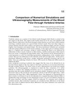
Figure 4.5 shows the proximal areas for the four major cities in northeast China.
One may also derive the proximal areas based on Euclidean distances and compare
the result to Figure 4.5.
4.4.2 PART 2: DEFINING HINTERLANDS BY THE HUFF MODEL
The procedures are similar to those in case study 4A, Part 2.
1. Measuring potential: Join the attribute table of city4 to the distance
table dist.dbf so that the information for city sizes is attached to the
distance table. Add a new field potent to dist.dbf, and calculate it
as potent = popu_nonfarm/RoadDist^2.
TABLE 4.2
Four Major Cities and Hinterlands in Northeast China
Major City Nonfarm Population

No. of Counties
Proximal Areas Huff Model
Dalian 1,661,127 7 7
Shenyang 3,054,868 72 72
Changchun 2,192,320 32 24
Harbin 2,990,921 92 100
2795_C004.fm Page 69 Friday, February 3, 2006 12:21 PM
© 2006 by Taylor & Francis Group, LLC
70 Quantitative Methods and Applications in GIS
2. Identifying cities with the highest potential: For the purpose of this project,
we only need to identify which city (among four major cities) exerts the
highest influence (potential) on a county, i.e., the maximum for
FIGURE 4.5 Proximal areas for four major cities in northeast China.
Harbin
Dalian
Shenyang
Changchun
Major city
Province
Proximal areas
Dalian
Shenyang
Changchun
Harbin
0 120 240 360 48060
Kilometers
Bohai
Sea
Heilongjiang
Prov.

Jilin Prov.
Liaoning
Prov.
Zhaoyuan county
N
Sd
jij
−β
2795_C004.fm Page 70 Friday, February 3, 2006 12:21 PM
© 2006 by Taylor & Francis Group, LLC
GIS-Based Trade Area Analysis and Applications in Geography and Planning 71
j = 1, 2, 3, and 4. For a particular county i, the denominator
in Equation 4.6 is the same for any city j; thus, the highest potential
implies the highest probability, i.e., .
On the table dist.dbf, use the tool Summarize to extract the maximum
potent by counties (i.e., INPUT_FID) and save the result as
max_potent.dbf. Join the table max_potent.dbf back to
dist.dbf, select records with the criterion dist.potent =
max_potent.max_potent, and export to a table Maxinfcity.dbf.
The output table Maxinfcity.dbf identifies which city has the highest
influence (potential) on each county.
3. Mapping hinterlands of major cities: Join the table MaxinfCity.dbf
to the county centroid shapefile CntyNEpt and then to the county poly-
gon layer cntyne for mapping. Figure 4.6 shows the hinterlands of four
major cities in northeast China by the Huff model.
4.4.3 DISCUSSION
Two observations can be made in Figure 4.5. First, a county (Zhaoyuan) in southwest
Heilongjiang Province appears closer to Harbin than to Changchun, but is in the
proximal area of Changchun based on the railroad distances. This becomes evident
by examining the railroad network in Figure 2.2. Second, some counties at the

southwest corner of the study area are closer to Dalin than to Shenyang in terms of
Euclidean distances but not by railroads. If the proximal areas were based on Euclid-
ean distances, these counties would be assigned to the hinterland of Dalian. Histor-
ically, these counties have closer economic ties with Shenyang, and thus belong to
its hinterland. This clearly demonstrates the advantage of using network distances
for measuring proximity. However, an important developing trend is the rising role
of waterway transportation across the Bohai Sea, and this may enhance the economic
linkage between these counties and Dalin and change the current boundaries of
hinterlands based on the railroads. Figure 4.6 is based on the Huff model accounting
for the impact of city sizes. Compared to Figure 4.5, the hinterlands of Shenyang
and Dalian are the same as those defined by the proximal area method. However,
Figure 4.6 shows an expanded hinterland of Harbin to include some counties closer
to Changchun, reflecting the impact of a larger population size of Harbin.
4.5 CONCLUDING REMARKS
While the concepts of proximal area method and the Huff model are straightforward,
their successful implementation relies on adequate measurements of variables, which
remains one of the most challenging tasks in trade area analysis.
First, both methods use distance or time. The proximal area method is based on
the commonly known least-effect principle in geography (Zipf, 1949). As shown in
case study 4B, road network distance or travel time is generally a better measure
()Sd
kik
k
n
−
=
∑
β
1
PSd Sd

ij j ij k ik
k
n
=
−−
=
∑
ββ
/( )
1
2795_C004.fm Page 71 Friday, February 3, 2006 12:21 PM
© 2006 by Taylor & Francis Group, LLC
72 Quantitative Methods and Applications in GIS
than straight-line (Euclidean) distance. However, network distance or travel time
may not be the best measure for travel impedance. Travel cost, convenience, comfort,
or safety may also be important. Research indicates that people of various socio-
economic or demographic characteristics perceive the same distance differently, i.e.,
FIGURE 4.6 Hinterlands for four major cities in northeast China by Huff model.
Harbin
Dalian
Shenyang
Changchun
Major city
Province
Hinterlands
Dalian
Shenyang
Changchun
Harbin
0 120 240 360 480 60

Kilometers
Bohai
Sea
Heilongjiang
Prov.
Jilin Prov.
Liaoning
Prov.
N
2795_C004.fm Page 72 Friday, February 3, 2006 12:21 PM
© 2006 by Taylor & Francis Group, LLC
GIS-Based Trade Area Analysis and Applications in Geography and Planning 73
a difference between cognitive and physical distances (Cadwallader, 1975). Defining
network distance or travel time also depends on the particular transportation mode.
Case study 4B uses railway, as it is currently the dominant mode for both passenger
and freight transportation in China. Similar to the U.S. experience, both air and
highway transportations are gaining more ground in China, and waterway can be
important in some areas. This makes distance or time measurement more than a
routine task. Accounting for interactions by telecommunication, Internet, and other
modern technologies adds further complexity to the issue.
Second, in addition to distance or time, the Huff model has two more variables:
attraction and travel friction coefficient (S and β in Equation 4.6). Attraction is
measured by winning percentage in case study 4A and population size in case study
4B. Both are oversimplification. More advanced methods may be employed to
consider more factors in measuring the attraction (e.g., the multiplicative competitive
interaction or MCI model). The travel friction coefficient β is also difficult to define,
as it varies across time and space, between transportation modes, and is dependent
on type of commodities, etc. For additional practice of trade area analysis methods,
one may conduct the trade area analysis of chain stores in a familiar study area.
Store addresses can be found on the Internet or in other sources (yellow pages, store

directories) and geocoded by the procedure discussed in case study 4A. Population
census data can be used to measure customer bases. A trade area analysis of the
chain stores may be used to project market potentials and evaluate the performance
of individual stores.
APPENDIX 4: ECONOMIC FOUNDATION OF THE GRAVITY MODEL
The gravity model is often criticized, particularly by economists, for its lack of foun-
dation in individual behavior. This appendix follows the work of Colwell (1982) in an
attempt to provide a theoretical base for the gravity model. For a review of other
approaches to derive the gravity model, see Fotheringham et al. (2000, pp. 217–234).
Assume a trip utility function in a Cobb–Douglas form, such as
(A4.1)
where u
i
is the utility of an individual at location i, x is a composite commodity
(i.e., all other goods), z is leisure time, t
ij
is the number of trips taken by an individual
at i to j, is the trip elasticity of utility that is directly related to the
destination population P
j
and reversely related to the origin population P
i
, and α, β,
γ, φ, and ζ are positive parameters. Colwell (1982, p. 543) justifies the particular
way of defining trip elasticity of utility on the ground of central place theory: larger
places serve many of the same functions as smaller places, plus higher-order func-
tions not found in smaller places; thus, the elasticity is larger for trips from the
smaller to the larger place than for trips from the larger to the smaller place.
The budget constraint is written as
(A4.2)

uaxzt
iij
ij
=
αγ
τ
τβ
ϕ
ξ
ij j i
PP= /
τ
ij
px rd t wW
ij ij
+=
2795_C004.fm Page 73 Friday, February 3, 2006 12:21 PM
© 2006 by Taylor & Francis Group, LLC
74 Quantitative Methods and Applications in GIS
where p is the price of x, r is the unit distance cost for travel, d
ij
is the distance
between point i and j, w is the wage rate, and W is the time worked.
In addition, the time constraint is
(A4.3)
where s is the time required per unit of x consumed, h is the travel time per unit of
distance, and H is total time.
Combining the two constraints in Equations A4.2 and A4.3 yields
(A4.4)
Maximizing the utility in Equation A4.1 subject to the constraint in Equation

A4.4 yields the following Lagrangian function:
Based on the four first-order conditions, i.e., ∂L/∂x = ∂L/∂z = ∂L/∂t
ij
= ∂L/∂λ = 0,
we can solve for t
ij
by eliminating λ, x, and z:
(A4.5)
It is assumed that travel cost per unit of distance r is a function of distance d
ij
,
such as
(A4.6)
where r
0
> 0 and σ > –1, so that total travel costs are an increasing function of
distance. Therefore, the travel time per unit of distance, h, has a similar function:
(A4.7)
so that travel time is proportional to travel cost. For simplicity, assume that the utility
function is homogeneous to degree 1, i.e.,
(A4.8)
Substituting Equations A4.6, A4.7, and A4.8 into Equation A4.5 and using
, we obtain
sx hd t z W H
ij ij
+++=
()( )p ws x rd whd t wz wH
ij ij ij
+++ +=
L ax z t p ws x rd whd t wz

ij ij ij ij
ij
=−++++−
αγ
τ
λ[( ) ( ) wwH]
t
wH
rwhd
ij
ij
ij ij
=
+++
τ
αγτ()( )
rrd
ij
=
0
σ
hhd
ij
=
0
σ
αγτ++ =
ij
1
τβ

ϕ
ξ
ij j i
PP= /
2795_C004.fm Page 74 Friday, February 3, 2006 12:21 PM
© 2006 by Taylor & Francis Group, LLC
GIS-Based Trade Area Analysis and Applications in Geography and Planning 75
(A4.9)
Finally, multiplying Equation A4.9 by the origin population yields the total
number of trips from i to j:
(A4.10)
which resembles the gravity model in Equation 4.14.
NOTES
1. The coverage of Thiessen polygons is based on the points from which it is generated,
and its extent may not cover all consumer locations.
2. Evidently this is an oversimplification. Despite their subpar records for many years,
the Cubs have earned the nickname “lovable losers,” as one of the most followed
clubs in professional sports. However, the record still matters, as tickets to Wrigley
Field became harder to get in 2004 after a rare play-off run by the Cubs in 2003.
This became more ironic in 2005 when the White Sox earned the best record in the
American League and eventually won the World Series.
3. Alternatively, in ArcToolBox, Geocoding Tools > Create Address Locator. However,
the interface in ArcCatalog is recommended as it provides more options.
4. One may also use the shapefile chitrtcent (population-weighted tract centroids)
provided in the CD. Section 5.4.1 discusses how the shapefile is obtained.
5. This is also close to
β
= 2.1, a value obtained by Yang (1990) in his study of gravity
models for analyzing the interregional passenger flow patterns in China.
6. One may need to export the combined table from the first join, and then join the

exported table to the polygon layer so that the fields contained in NearCity_id.dbf
will not be lost in the second join.
t
wH P P
rwhd
ij
ij
ij
=
+
−
+
β
ξ
ϕ
σ
()
00
1
TPt
wH P P
rwhd
ij i ij
ij
ij
==
+
−
+
β

ξ
ϕ
σ
1
00
1
()
2795_C004.fm Page 75 Friday, February 3, 2006 12:21 PM
© 2006 by Taylor & Francis Group, LLC