Quantitative Methods and Applications in GIS - Chapter 8 pps
Bạn đang xem bản rút gọn của tài liệu. Xem và tải ngay bản đầy đủ của tài liệu tại đây (916 KB, 19 trang )
Part III
Advanced Quantitative Methods
and Applications
2795_S003.fm Page 265 Friday, February 3, 2006 11:57 AM
149
8
Geographic Approaches
to Analysis of Rare Events
in Small Population and
Application in Examining
Homicide Patterns
When rates are used as estimates for an underlying risk of a rare event (e.g., cancer,
AIDS, homicide), those with a small base population have high variance and are
thus less reliable. The spatial smoothing techniques, such as the floating catchment
area method and the empirical Bayesian smoothing method, as discussed in
Chapter 2, can be used to mitigate the problem. This chapter begins with a survey
of various approaches to the problem of analyzing rare events in a small population
in Section 8.1. Two geographic approaches, namely, the ISD method and the spatial-
order method, are fairly easy to implement and are introduced in Section 8.2. The
spatial clustering method based on the scale-space theory requires some program-
ming and is discussed in Section 8.3. In Section 8.4, the case study of analyzing
homicide patterns in Chicago is presented to illustrate the scale-space melting
method implemented in Visual Basic. The section also provides a brief review of
the substantive issues: job access and crime patterns. The chapter is concluded in
Section 8.5 with a brief summary.
8.1 THE ISSUE OF ANALYZING RARE EVENTS IN A
SMALL POPULATION
Researchers in criminology and health studies and others are often confronted with
the task of analyzing rare events in a small population and have long sought solutions
to the problem.
For criminologists, the study of homicide rates across geographic units and for
demographically specific groups often entails analysis of aggregate homicide rates
in small populations. Several nongeographic strategies have been attempted by
criminologists to mitigate the problem. For example, Morenoff and Sampson (1997)
used homicide counts instead of per capita rates or simply deleted outliers or
unreliable estimates in areas with a small population. Some used larger units of
analysis (e.g., states, metropolitan areas, or large cities) or aggregated over more
years to generate stable homicide rates. Land et al. (1996) and Osgood (2000) used
2795_C008.fm Page 149 Friday, February 3, 2006 12:13 PM
150
Quantitative Methods and Applications in GIS
Poisson-based regressions to better capture the nonnormal error distribution pattern
in regression analysis of homicide rates in small populations (see Appendix 8).
1
On the other side, many researchers in health-related fields are well trained in
geography and have used several spatial analytical or geographic methods to address
the issue. Geographic approaches aim at constructing larger geographic areas, based
on which more stable rate estimates may be obtained. The purpose of constructing
larger geographic areas is similar to that of aggregating over a longer period of time:
to achieve a greater degree of stability in homicide rates across areas. The technique
has much common ground with the long tradition of regional classification
(
regionalization
) in geography (Cliff et al., 1975). For instance, Black et al. (1996)
developed the
ISD method
(after the Information and Statistics Division of the Health
Service in Scotland, where it was devised) to group a large number of census
enumeration districts (EDs) in the U.K. into larger analysis units of approximately
equal population size. Lam and Liu (1996) used the
spatial-order method
to generate
a national rural sampling frame for HIV/AIDS research, in which some rural counties
with insufficient HIV cases were merged to form larger sample areas. Both
approaches emphasize spatial proximity, but neither considers within-area homo-
geneity of attribute. Haining et al. (1994) attempted to consolidate many EDs in the
Sheffield Health Authority Metropolitan District in the U.K. to a manageable number
of regions for health service delivery (hereafter referred to as the Sheffield method).
The Sheffield method started by merging adjacent EDs sharing similar deprivation
index scores (i.e., complying with
within-area attribute homogeneity
), and then used
several subjective rules and local knowledge to adjust the regions for spatial com-
pactness (i.e., accounting for
spatial proximity
). The method attempted to balance
two criteria (attribute homogeneity and spatial proximity), a major challenge in
regionalization analysis. In other words, only contiguous EDs can be clustered
together, and these EDs must have similar attributes.
The ISD method and the spatial-order method will be discussed in Section 8.2
in detail. The Sheffield method relies on subjective criteria and involves a substantial
amount of manual work that requires one’s knowledge of the study area. Section
8.3 will introduce a new spatial clustering method based on the scale-space theory.
The method melts adjacent polygons of similar attributes into clusters like the
Sheffield method, but is an automated process based on objective criteria. Construct-
ing geographic areas enables the analysis to be conducted at multiple geographic
levels, and thus permits the test of the
modifiable areal unit problem
(MAUP).
Table 8.1 summarizes all approaches to the problem of analysis of rates of rare
events in a small population.
8.2 THE ISD AND THE SPATIAL-ORDER METHODS
The ISD method is illustrated in Figure 8.1 (based on Black et al., 1996, with
modifications). A starting polygon (e.g., the southernmost one) is selected first, and
its nearest and contiguous polygon is added. If the total population is equal to or
more than the threshold population, the two polygons form an analysis area.
Otherwise, the next nearest polygon (contiguous to either of the previous selected
polygons) is added. The process continues until the total population of selected
2795_C008.fm Page 150 Friday, February 3, 2006 12:13 PM
Geographic Approaches to Analysis of Rare Events and Homicide Patterns
151
polygons reaches the threshold value and a new analysis area is formed. The whole
procedure is repeated until all polygons are allocated to new analysis areas. One
may use ArcGIS to generate a matrix of distances between polygons and another
matrix of polygon adjacency, and then write a simple computer program to imple-
ment the method outside of GIS (e.g., Wang and O’Brien, 2005). The method is
primitive and does not account for spatial compactness. Some analysis areas
TABLE 8.1
Approaches to Analysis of Rates of Rare Events in a Small Population
Approach Examples Comments
1 Use homicide counts
instead of per capita
rates
Morenoff and Sampson (1997) Not applicable for most studies that
are interested in the offense or
victimization rate relative to
population size
2 Delete samples of
small populations
Harrell and Gouvis (1994);
Morenoff and Sampson (1997)
Deleted observations may contain
valuable information
3 Aggregate over more
years or to a high
geographic level
Messner et al. (1999); most
studies surveyed by Land et al.
(1990)
Impossible to analyze variations
within the time period or within the
large areal unit
4 Poisson-based
regressions
Osgood (2000); Osgood and
Chambers (2000)
Effective remedy for OLS
regressions; not applicable to
nonregression studies
5 Construct geographic
areas with large
enough populations
Haining et al. (1994); Black et al.
(1996); Sampson et al. (1997)
Generate reliable rates for statistical
reports, mapping, regression
analysis, and others
FIGURE 8.1
The ISD method.
Select starting tract from pool of unallocated tracts
Add to analysis areas;
remove from pool
Is population of analysis
area ≥ threshold
e analysis area
completed
Select the tract
contiguous & nearest
Are all tracts allocated?
Yes
Yes
No
No
Stop
2795_C008.fm Page 151 Friday, February 3, 2006 12:13 PM
152
Quantitative Methods and Applications in GIS
generated by the method may exhibit odd shapes, and some (particularly those near
the boundaries) may require manual adjustment.
The spatial-order method follows a rationale similar to that of the ISD method. It
uses space-filling curves to determine the nearness or spatial order of polygons. Space-
filling curves traverse space in a continuous and recursive manner to visit all polygons,
and assign a spatial order (from 0 to 1) to each polygon based on its relative positions
in a two-dimensional space. The procedure, currently available in ArcInfo Workstation,
is SPATIALORDER, based on one of the algorithms developed by Bartholdi and
Platzman (1988). In general, polygons that are close together have similar spatial-
order values and polygons that are far apart have dissimilar spatial-order values.
See Figure 8.2 for an example. The method provides a first-cut measure of closeness.
The SPATIALORDER command is available in the ArcPlot module through the
ArcInfo Workstation command interface. Once the spatial-order value of each polygon
is determined, the COLLOCATE command in ArcInfo follows by assigning nearby
polygons one group number and accounting for the capacity of each group formed by
polygons. Finally, polygons are dissolved based on the group numbers.
8.3 THE SCALE-SPACE CLUSTERING METHOD
The ISD and the spatial-order method only consider spatial proximity, but not within-
area attribute homogeneity. The spatial clustering method based on the scale-space
theory accounts for both criteria. Development of the scale-space theory has bene-
fited from the advancement of computer image processing technologies, and most
of its applications are in analysis of remote sensing data. Here we use the method
for addressing the issue of analyzing rare events in small populations.
FIGURE 8.2
An example for assigning spatial-order values to polygons.
Spatial order value
0.0 0.5 1.0
6
1
2
3, 5
4
10, 8, 7
9
Node ID
10
0.656
9
0.880
8
0.687
7
0.688
4
0.582
3
0.361
5
0.371
6
0.080
1
0.157
2
0.202
2795_C008.fm Page 152 Friday, February 3, 2006 12:13 PM
Geographic Approaches to Analysis of Rare Events and Homicide Patterns
153
As we know, objects in the world appear in different ways depending upon the
scale of observation. In the case of an image, the size of scale ranges from a single
pixel to a whole image. There is no right scale for an object, as any real-world object
may be viewed at multiple scales. The operation of systematically simplifying an
image at a finer scale and representing it at coarser levels of scale is termed
scale-
space smoothing
. A major reason for scale-space smoothing is to suppress and
remove unnecessary and disturbing details (Lindeberg, 1994, p. 10). There are
various scale-space clustering algorithms (e.g., Wong, 1993; Wong and Posner,
1993). In essence, an image is composed of many pixels with different brightness.
As the scale increases, smaller pixels are melted to form larger pixels. The melting
process is guided by some objectives, such as entropy maximization (i.e., minimizing
loss of information). Applying the scale-space clustering method in a socioeconomic
context requires simplification of the algorithm.
The procedures below are based on Wang (2005). The idea is that major features
of an image can be captured by its brightest pixels (represented as local maxima).
By merging surrounding pixels (up to local minima) to the local maxima, the image
is simplified with fewer pixels while the structure is preserved. Five steps implement
the concept:
1.
Draw a link between each polygon and its most similar adjacent polygon
:
A polygon
i
has
t
attributes (
x
i
1
, …,
x
it
), and its adjacent polygons
j
(
j
= 1,
2, …,
m
) have attributes (
x
j
1
, …,
x
jt
). Attributes
x
it
and
x
jt
are standardized.
Polygon
i
is linked to only polygon
k
among its adjacent polygons
j
based
on the rook contiguity (sharing a boundary, not only a vertex) if
, i.e., the minimum distance criterion.
2
As a
result, a link is established between each polygon and one of its adjacent
polygons with the most similar attributes.
2.
Determining the link’s direction
: The direction of the link between poly-
gons
i
and
k
is determined by their attribute values, represented by an
aggregate score (
Q
). In the case study in Section 8.4.,
Q
is the average of
three factor scores weighted by their corresponding eigenvalues (repre-
senting proportions of variance captured by the factors). Higher scores of
any of the three factors indicate more socioeconomic disadvantages. The
direction is defined such as
i
→
k
or
L
ik
= 1 if
Q
i
<
Q
k
; otherwise,
i
←
k
or
L
ik
= 0. Therefore, the directional link always points toward a higher
aggregate score. For instance, in Figure 8.3, the arrow points to polygon
1 for the link between 1 and 2 because
Q
2
<
Q
1
.
3.
Identifying local minima and maxima
: A local minimum (maximum) is a
polygon with all directional links pointing toward other polygons (itself),
i.e., with the lowest (highest)
Q
among surrounding polygons.
4.
Grouping around local maxima
: Beginning with a local minimum, search
outward following link directions until a local maximum is reached. All
polygons between the local minimum and maximum are grouped into one
cluster. If other local minima are also linked to the same local maximum,
all polygons along the routes are also grouped into the same cluster. This
step is repeated until all polygons are grouped.
D
xx
ik j
m
it jt
t
=−
∑
min { ( ) }
2
2795_C008.fm Page 153 Friday, February 3, 2006 12:13 PM
154
Quantitative Methods and Applications in GIS
5.
Continuing the next-round clustering
: Steps 1 to 4 yield the result of the
first round of clustering, and each cluster can be represented by the
averaged attributes of composed polygons (weighted by each polygon’s
population). The result is fed back to step 1, which begins another round
of grouping. The process may be repeated until all units are grouped into
one cluster.
Now we use a simple example shown in Figure 8.3 to explain the process. In
step 1, polygon 1 is linked to both 2 and 3. Polygons 1 and 3 are linked because 3
is the polygon most similar to 1 between polygon 1’s adjacent polygons 2 and 3,
but the link between polygons 1 and 2 is established because 1 is the polygon most
similar to 2 among polygon 2’s adjacent polygons 1, 3, 9, and 4. Similarly, polygon 4
is linked to both 5 and 7, but 5 is the polygon most similar to 4 among polygon 4’s
adjacent polygons 2, 9, 5, and 7, and 4 is the polygon most similar to 7 among
polygon 7’s adjacent polygons 4, 5, and 8. Step 2 computes the values of
Q
for all
polygons. In step 3, polygons 2, 3, 4, and 9 are all initially identified as local minima,
as all the links are pointed outward there; polygons 1, 6, and 8 are all local maxima,
as all the links are pointed inward there. In step 4, both polygons 2 and 3 point to 1,
and they are grouped into cluster I; polygons 4 and 9 point to 5 and then to 6, and
they are all grouped into cluster II. By doing so, any local maximum (the brightest
pixel) serves as the center of a cluster, and surrounding polygons (with less bright-
ness) are melted into the cluster. The cluster stops until it reaches local minima
(with the least brightness). The process is repeated until all polygons are grouped.
FIGURE 8.3
An example of clustering based on the scale-space theory.
1
5
6
8
3
2
4
1, 2, : Tract No.
Local maximum
Link’s direction
Tract boundary
Cluster boundary
I
II
7
Local minimum
9
III
I, II, : Cluster No.
2795_C008.fm Page 154 Friday, February 3, 2006 12:13 PM
Geographic Approaches to Analysis of Rare Events and Homicide Patterns
155
Note that in Figure 8.3, polygon 4 points to two polygons 5 and 7, but it follows
the link to 5 instead of the link to 7 to begin the melting process, as polygon 5 is
the most similar one among polygon 4’s four adjacent polygons (the link between 4
and 7 is established because 4 is polygon 7’s most similar adjacent polygon). Once
polygon 4 is melted to cluster II, the link between 4 and 7 becomes redundant and
is indicated as a broken link in dashed line, and polygon 7 becomes a new local
minimum (indicated in a dashed box). Polygons 7 and 8 are thus grouped together
to form cluster III. Also refer to Figure 8.6 for a sample area illustrating the
melting process.
The spatial clustering method based on the scale-space theory is implemented
in the program file
Scalespace.dll
, developed in Visual Basic.
3
The file is
attached in the CD, and its usage is illustrated in the next section. The process may
be repeated to generate multiple levels of clustering.
8.4 CASE STUDY 8: EXAMINING THE RELATIONSHIP
BETWEEN JOB ACCESS AND HOMICIDE PATTERNS IN
CHICAGO AT MULTIPLE GEOGRAPHIC LEVELS BASED ON
THE SCALE-SPACE MELTING METHOD
Most crime theories suggest, or at least imply, an inverse relationship between legal
and illegal employment. The
strain theory
(e.g., Agnew, 1985) argues that crime
results from the inability to achieve desired goals, such as monetary success, through
conventional means like legitimate employment. The
control theory
(e.g., Hirschi,
1969) suggests that individuals unemployed or with less desirable employment have
less to lose by engaging in crime. The
rational choice
(e.g., Cornish and Clarke,
1986) and
economic
(e.g., Becker, 1968)
theories
argue that people make rational
choices to engage in a legal or illegal activity by assessing the cost, benefit, and risk
associated with it. Research along this line has focused on the relationship between
unemployment
and crime rates (e.g., Chiricos, 1987). According to the economic
theories, job market probably affects economic crimes (e.g., burglary) more than
violent crimes, including homicide (Chiricos, 1987). Support for the relationship
between job access and homicide can be found in the
social stress theory
. According
to the theory, “high stress can indicate the lack of access to basic economic resources
and is thought to be a precipitator of … homicide risk” (Rose and McClain, 1990,
pp. 47–48). Social stressors include any psychological, social, and economic factors
that form “an unfavorable perception of the social environment and its dynamics,”
particularly unemployment and poverty, which are explicitly linked to social prob-
lems, including crime (Brown, 1980).
Most literature on the relation between job market and crime has focuses on the
link between unemployment and crime using large areas such as the whole nation,
states, or metropolitan areas (Levitt, 2001). There may be more variation
within
such
units than
between
them. Recent advancements have been made by analyzing the
relationship between local job market and crime (e.g., Bellair and Roscigno, 2000).
Wang and Minor (2002) argued that not every job is an economic opportunity for
all, and only an accessible job is meaningful. They proposed that
job accessibility
,
2795_C008.fm Page 155 Friday, February 3, 2006 12:13 PM
156
Quantitative Methods and Applications in GIS
reflecting one’s ability to overcome spatial and other barriers to employment, was
a better measure of local job market condition. Their study in Cleveland suggested
a reverse relationship between job accessibility and crime, and stronger (negative)
relationships with economic crimes (including auto theft, burglary, and robbery)
than violent crimes (including aggravated assault, homicide, and rape). Wang (2005)
further extended the work to focus on the relationship between job access and
homicide patterns with refined methodology, based on which this case study is
developed. The study focused on homicides for two reasons. First, homicide is
considered the most accurately reported crime rate for interunit comparison (Land
et al., 1990, p. 923). Second, homicide is rare, and analysis of homicide in small
populations makes a good example to illustrate the methodological issues empha-
sized by this chapter.
This case study uses OLS regressions to examine the possible association
between job access and homicide rates in Chicago while controlling for socioeco-
nomic covariates. Case study 9C in Section 9.6 will use spatial regressions to account
spatial autocorrelation.
The following datasets are provided in the CD for this project:
1. A polygon coverage
citytrt
contains 845 census tracts (excluding
one polygon without any tract code or residents) in the city of Chicago
(excluding the O’Hare tract because of its unique land use and noncon-
tiguity with other tracts)
2. A text file
cityattr.txt
contains tract IDs and 10 corresponding
socioeconomic attribute values based on the 1990 Census.
3. A program file
Scalespace.dll
implements the scale-space cluster-
ing tool.
In the attribute table of coverage
citytrt
, the item
cntybna
is each tract’s
unique ID, the item
popu
is population in 1990, the item
JA
is job accessibility
measured by the methods discussed in Chapter 4 (a higher
JA
value corresponds to
better job accessibility), and the item
CT89_91
is total homicide counts for a 3-year
period around 1990 (i.e., 1989 to 1991). Homicide data for the study area are
extracted from the 1965 to 1995 Chicago homicide dataset compiled by Block et
al. (1998), available through the National Archive of Criminal Justice Data (NACJD)
at www.icpsr.umich.edu/NACJD/home.html. Homicide counts over a period of
3 years are used to help reduce measurement errors and stabilize rates. In addition,
for convenience it also contains the result from the factor analysis (implemented in
step 0 below):
factor1
,
factor2
, and
factor3
are scores of three factors that
have captured most of the information contained in the socioeconomic attribute file
cityattr.txt
. Note that the job market for defining job accessibility is based
on a much wider area (six mostly urbanized counties: Cook, DuPage, Kane, Lake,
McHenry, and Will) than the city of Chicago.
Data for defining the 10 socioeconomic variables and population are based on the
STF3A files from the 1990 Census and are measured in percentage. In the text file
cityattr.txt
, the first column is tract IDs (i.e., identical to the item
cntybna
in the GIS layer
citytrt
) and the 10 variables are in the following order:
2795_C008.fm Page 156 Friday, February 3, 2006 12:13 PM
Geographic Approaches to Analysis of Rare Events and Homicide Patterns
157
1. Families below the poverty line (labeled “poverty” in Table 8.2)
2. Families receiving public assistance (“public assistance”)
3. Female-headed households with children under 18 (“female-headed
households”)
4. “Unemployment”
5. Residents who moved in the last 5 years (“new residents”)
6. Renter-occupied homes (“renter occupied”)
7. Residents without high school diplomas (“no high school diploma”)
8. Households with an average of more than 1 person per room (“crowdedness”)
9. Black residents (“black”)
10. Latino residents (“Latinos”)
0. Optional:
Factor analysis on socioeconomic covariates
: Use SAS or other
statistical software to conduct factor analysis based on the 10 socioeconomic
covariates contained in
cityattr.txt
. Save the result (factor scores and
the tract IDs) in a text file and attach it to the GIS layer. This step provides
another practice opportunity for principal components and factor analysis,
discussed in Chapter 7. Refer to Appendix 7B for a sample SAS program
containing a factor analysis procedure. It is optional, as the result (factor
scores) is already provided in the polygon coverage
citytrt
.
The principal components analysis result shows that three components
(factors) have eigenvalues greater than 1 and are thus retained. These three
factors capture 83% of the total variance of the original 10 variables.
Table 8.2 shows the rotated factor patterns. Factor 1 (accounting for 56.6%
variance among three factors) is labeled “concentrated disadvantage” and
captures five variables (public assistance, female-headed households, black,
poverty, and unemployment). Factor 2 (accounting for 26.6% variance
among three factors) is labeled “concentrated Latino immigration” and
captures three variables (residents with no high school diplomas, households
TABLE 8.2
Rotated Factor Patterns of Socioeconomic Variables in Chicago 1990
Factor 1 Factor 2 Factor 3
Public assistance 0.93120 0.17595 –0.01289
Female-headed households 0.89166 0.15172 0.16524
Black 0.87403 –0.23226 –0.15131
Poverty 0.84072 0.30861 0.24573
Unemployment 0.77234 0.18643 –0.06327
Non-high school diploma 0.40379 0.81162 –0.11539
Crowdedness 0.25111 0.83486 –0.12716
Latinos –0.51488
0.78821 0.19036
New residents –0.21224 –0.02194 0.91275
Renter occupied 0.45399 0.20098 0.77222
2795_C008.fm Page 157 Friday, February 3, 2006 12:13 PM
158 Quantitative Methods and Applications in GIS
with more than one person per room, and Latinos). Factor 3 (accounting
for 16.7% variance among three factors) is labeled “residential instability”
and captures two variables (residential instability and renter-occupied
homes). The three factors are used as control variables (socioeconomic
covariates) in the regression analysis of job access and homicide rate. The
higher the value of each factor is, the more disadvantageous a tract is in
terms of socioeconomic characteristics.
1. Creating the shapefile with valid census tracts: Open the coverage
citytrt in ArcMap > Use Select by Attributes to select polygons with
popu > 0 (845 tracts selected) > Export to a shapefile citytract.
2. Computing homicide rates: Because of rarity of the incidence, homicide
rates are usually measured as homicides per 100,000 residents. Open the
shapefile citytract in ArcMap and open its attribute table > Add a field
homirate to the table, and calculate it as homirate = CT89_91
*100000/popu. The rate is measured as per 100,000 residents.
In regression analysis, the logarithmic transformation of homicide rates
(instead of the raw homicide rate) is often used to measure the dependent
variable (see Land et al., 1990, p. 937), and 1 is added to the rates to
avoid taking the logarithm of zero.
4
Add another field, Lhomirat, to the
attribute table of shapefile citytract and calculate it as Lhomirat
= log(homirate+1).
3. Mapping tracts with small population: Figure 8.4 shows that 74 census
tracts have a population of fewer than 500, and 28 tracts fewer than 100.
Check the raw homicide rate, homirate, in these small-population
tracts, and note that some tracts have very high rates. This highlights the
problem of unstable rates in small populations.
4. Regression analysis at the census tract level: Use Microsoft Excel or SAS
to run an OLS regression at the census tract level: the dependent variable
is Lhomirat and the explanatory variables are JA, factor1,
factor2, and factor3. Refer to Section 6.5.1 if necessary. The result
is shown in Table 8.3.
5. Installing the scale-space clustering tool: In ArcMap, choose Tools >
Customize > click the Command tab > choose “Add from file,” browse
to the ScaleSpace.dll file saved under your project directory, and
open it > still with the Command tab clicked in the same dialog window,
find and click Scale-Space Tool under Categories to install it.
6. Using the clustering tool to obtain first-round clusters: Click the
button from ArcMap to access the “scale-space cluster” tool and activate
the dialog window. Define the choices in the dialog as shown in Figure
8.5. The input shapefile is citytract. Use arrows to move variables
factor1, factor2, and factor3 to the column of “selected fields,”
which are used as criteria measuring the attribute similarity among
tracts. Input their corresponding weights: 0.566, 0.266, and 0.167 (based
on the percentage of variance captured by each factor). Use the variable
POPU as the weight field to compute weighted averages of attributes in
2795_C008.fm Page 158 Friday, February 3, 2006 12:13 PM
Geographic Approaches to Analysis of Rare Events and Homicide Patterns 159
the clusters to be formed. The field for the cluster membership in the
input shapefile may be named Clus1 (or others). Define the output
directory and the shapefile name (e.g., Cluster1 by default). One may
also check the two boxes for showing and saving intermediate results,
and name the shapefile identifying the local minima and local maxima
and the shapefile for link directions and types. Finally, click OK to
execute the analysis.
FIGURE 8.4 Census tracts with small populations in Chicago 1990.
0121.5
Kilometers
Legend
Census tract
POPU
30–100
101–500
501–17728
N
963
2795_C008.fm Page 159 Friday, February 3, 2006 12:13 PM
160 Quantitative Methods and Applications in GIS
TABLE 8.3
OLS Regression Results from Analysis of Homicide
in Chicago 1990
Census Tracts First-Round Clusters
No. of observations 845 316
Intercept 6.1324
(10.87)
***
6.929
(8.14)
***
Factor 1 1.2200
(15.43)
***
1.001
(8.97)
***
Factor 2 0.4989
(7.41)
***
0.535
(5.82)
***
Factor 3 –0.1230
(–1.84)
–0.283
(–2.93)
**
Job Accessibility (JA) –2.9143
(–5.41)
***
–3.230
(–3.97)
***
R
2
0.317 0.441
Note: t values in parentheses;
***
, significant at 0.001;
**
, significant
at 0.01;
*
, significant at 0.05.
FIGURE 8.5 Dialog window for the scale-space clustering tool.
2795_C008.fm Page 160 Friday, February 3, 2006 12:13 PM
Geographic Approaches to Analysis of Rare Events and Homicide Patterns 161
Figure 8.6 is the northeast corner of the study area showing the
clustering process and result. If no links are pointed from or toward
a tract (often as a result of broken links), it is an “orphan” and forms a cluster
itself. The clustering result is saved in the shapefile Cluster. Additional
fields are also created in the attribute table of shapefile citytract to save
some intermediate results in the clustering process, as well as the clus-
tering result. The attribute table of shapefile Cluster1 contains the
weighted averages of attribute variables factor1, factor2, and
factor3, as well as the weight field POPU. Figure 8.7 shows the result
of this first-round clustering. One may conduct further grouping based on
the shapefile Cluster1.
7. Aggregating data to the first-round clusters: Both the independent and
dependent variables (JA, factor1, factor2, factor3, and
homirate) need to aggregate to the cluster level (identified by the field
FIGURE 8.6 A sample area for illustrating the clustering process.
Legend
Min or max
Local minima
Local maxima
Orphan
Link type & direction
Regular link
Broken link
1st-round clusters
Census tracts
2795_C008.fm Page 161 Friday, February 3, 2006 12:13 PM
162 Quantitative Methods and Applications in GIS
Clus1) by calculating the weighted averages using the population
(popu) as weights.
5
Variables (e.g., factor1, factor2, factor3)
in the attribute table of shapefile Cluster1 are already the weighted
averages. This step shows how the computation is implemented in ArcMap
based on the attribute table of shapefile citytract. Taking factor1
as an example, this is achieved by three steps
6
: (a) calculating a field (say,
F1XP) as factor1 multiplied by popu, (b) computing the total
FIGURE 8.7 First-round clusters by the scale-space clustering method.
01
Kilometers
Legend
1st-round cluster
Census tract
2468
N
2795_C008.fm Page 162 Friday, February 3, 2006 12:13 PM
Geographic Approaches to Analysis of Rare Events and Homicide Patterns 163
population (say, sum_popu) and summing up the new field F1XP (say,
sum_F1XP) within each cluster, and (c) dividing sum_F1XP by
sum_popu to obtain the weighted value for factor1. In detail, it is
implemented as follows:
a. Add new fields F1XP, F2XP, F3XP, JAXP, and HMXP to the attribute
table of shapefile citytract and calculate each of them as:
F1XP=factor1*popu,
F2XP=factor2*popu,
F3XP=factor3*popu,
JAXP=JA*popu,
HMXP=homirate*popu;
b. Sum up these new fields (F1XP, F2XP, F3XP, JAXP, and HMXP) and
the field popu by clusters (i.e., the field Clus1), and name the output
file sum_clus1.dbf containing the cluster IDS (Clus1), number
of tracts within each cluster (count), and the summed-up fields
(Sum_F1XP, Sum_F2XP, Sum_F3XP, Sum_JAXP, Sum_HMXP,
Sum_popu).
c. Add new fields factor1, factor2, factor3, JA, and homirate
to the file sum_clus1.dbf and calculate each of them as:
factor1=Sum_F1XP/Sum_popu,
factor2=Sum_F2XP/Sum_popu,
factor3=Sum_F3XP/Sum_popu,
JA=Sum_JA/Sum_popu,
homirate=Sum_HMXP/Sum_popu;
Finally, add a field Lhomirat to sum_clus1.dbf and calculate it
as Lhomirat = log(homirate+1).
8. Regression analysis based on the first-round clusters: Run the OLS
regression in Excel or SAS using sum_clus1.dbf. The regression
result is also presented in Table 8.3.
The OLS regression results based on both the census tracts and first-round
clusters show that job accessibility is negatively related to homicide rates
in Chicago. Case study 9C in Section 9.6 will further examine the issue
while controlling for spatial autocorrelation.
8.5 SUMMARY
In geographic areas with few events (e.g., cancer, AIDS, homicide), rate estimates
are often unreliable because of random error associated with small numbers.
Researchers have proposed various approaches to mitigate the problem. Applications
are particularly rich in criminology and health studies. Among various methods,
geographic approaches seek to construct larger geographic areas so that more stable
2795_C008.fm Page 163 Friday, February 3, 2006 12:13 PM
164 Quantitative Methods and Applications in GIS
rates may be obtained. The ISD method and the spatial-order method are fairly
primitive and do not consider whether areas grouped together are homogenous in
attributes. The spatial clustering method based on the scale-space theory accounts
for attribute homogeneity while grouping adjacent geographic areas together. It is
inevitable that aggregation to larger geographic areas results in the loss of some of
the original detail. The scale-space melting process is guided by some objectives,
such as entropy maximization (i.e., minimizing loss of information). The method
treats a study area composed of many polygons as a picture of pixels. If the attributes
in each pixel may be summed up as a single index, this index can be regarded as a
measurement of brightness capturing the structure of a picture in black and white.
By grouping the pixels together around the brightest ones, fewer and larger pixels
are used to capture the basic structure of the original picture at a finer resolution.
A test version of this method is implemented in Visual Basic and incorporated
in the ArcGIS environment. The method is applied to examining homicide patterns
in Chicago and analyzing whether they are related to job access. The study shows
that poorer job access indeed is associated with higher homicide rates while con-
trolling for socioeconomic covariates.
APPENDIX 8: THE POISSON-BASED REGRESSION ANALYSIS
This appendix is based on Osgood (2000). Assuming the timing of the events is
random and independent, the Poisson distribution characterizes the probability of
observing any discrete number (0, 1, 2, …) of events for an underlying mean count.
When the mean count is low (e.g., in a small population), the Poisson distribution
is skewed toward low counts. In other words, only these low counts have meaningful
probabilities of occurrence. When the mean count is high, the Poisson distribution
approaches the normal distribution and a wide range of counts have meaningful
probabilities of occurrence.
The basic Poisson regression model is
(A8.1)
where λ
i
is the mean (expected) number of events for case i, x’s are explanatory
variables, and β’s are regression coefficients. Note that the left-hand side in Equation
A8.1 is the logarithmic transformation of the dependent variable. The probability of
an observed outcome y
i
follows the Poisson distribution, given the mean count λ
i
,
such as
(A8.2)
Equation A8.2 indicates that the expected distribution of crime counts depends on
the fitted mean count λ
i
.
ln( ) λββ β β
ikk
xx x=+ + ++
01122
Pr( )
!
Yy
e
y
ii
i
y
i
i
i
==
−λ
λ
2795_C008.fm Page 164 Friday, February 3, 2006 12:13 PM
Geographic Approaches to Analysis of Rare Events and Homicide Patterns 165
In many studies, it is the rates, not the counts, of events that are of most interest
to analysts. Denoting the population size for case i as n
i
, the corresponding rate is
. The regression model for rates is written as
i.e.,
(A8.3)
Equation A8.3 adds the population size n
i
(with a fixed coefficient of 1) to the
basic Poisson regression model (Equation A8.1) and transforms the model of ana-
lyzing counts to a regression model of analyzing rates. The model is a Poisson-based
regression that is standardized for the size of base population, and solutions can be
found in many statistical packages (e.g., LIMDEP).
Note that the variance of the Poisson distribution is the mean count λ, and thus
its standard deviation is . The mean count of events equals the underlying
per capita rate r multiplied by the population size n, i.e., . When a variable
is divided by a constant, its standard deviation is also divided by the constant.
Therefore, the standard deviation of rate r is
(A8.4)
Equation A8.4 shows that the standard deviation of per capita rate r is inversely
related to the population size n, i.e., the problem of heterogeneity of error variance
discussed in Section 8.1. The Poisson-based regression explicitly addresses the issue
by acknowledging the greater precision of rates in larger populations.
NOTES
1. Aggregate crime rates from small populations violate two assumptions of ordinary
least squares (OLS) regressions, i.e., homogeneity of error variance (because errors
of prediction are larger for crime rates in smaller populations) and normal error
distribution (because more crime rates of zero are observed as populations decrease).
2. Depending on the applications and the variables used, criteria defining attribute
similarity can be different. For example, in the study of regional partitioning of Jingsu
Province in China, Luo et al. (2002) computed the correlation coefficients between
a county and its adjacent counties and drew a link between the two with the highest
coefficient. Their goal was to group areas of a similar socioeconomic structure, i.e.,
grouping counties at lower development levels with central cities at higher develop-
ment levels, to form economic regions. As discussed in Section 7.2, there are also
different measures for distance.
3. The scale-space cluster tool was developed by Dr. Lan Mu at the Department of
Geography, University of Illinois–Urbana-Champaign.
λ
ii
n/
ln( / ) λβββ β
ii kk
nxxx=+ + ++
01122
ln( ) ln( ) λββββ
ii kk
nxxx=+++++
01122
SD
λ
λ=
λ=rn
SD SD n n rn n r n
r
====
λ
λ// //
2795_C008.fm Page 165 Friday, February 3, 2006 12:13 PM
166 Quantitative Methods and Applications in GIS
4. The choice of adding 1 (instead of 0.2, 0.5, or others) is arbitrary and may bias the
coefficient estimates. However, different additive constants have minimal conse-
quence for significance testing, as standard errors grow proportionally with the
coefficients and thus leave the t values unchanged (Osgood, 2000, p. 36). In addition,
adding 1 ensures that log(r + 1) = 0 for r = 0 (zero homicide).
5. In an updated version of program file Scalespace.dll, to be released soon, all
variables in the clusters are computed directly by the scale-space cluster tool.
6. In formula, the weighted average is .
xwxw
w
ii i
=
∑∑
()/
2795_C008.fm Page 166 Friday, February 3, 2006 12:13 PM