GIS Based Studies in the Humanities and Social Sciences - Chpater 16 pptx

229

16

Estimating Urban Agglomeration
Economies for Japanese Metropolitan Areas:

Is Tokyo Too Large?

Yoshitsugu Kanemoto, Toru Kitagawa, Hiroshi Saito, and Etsuro Shioji
CONTENTS

16.1 Introduction 229
16.2 Production Functions with Agglomeration Economies 230
16.3 Cross-Section Estimates 232
16.4 Panel Estimates 234
16.5 A Test for Optimal City Sizes 236
16.6 Conclusion 240
Acknowledgement 240
References 241

16.1 Introduction



Tokyo is Japan’s largest city, with a population currently exceeding 30 million
people. Congestion on commuter trains is almost unbearable, with the aver-
age time for commuters to reach downtown Tokyo (consisting of the three
central wards of Chiyoda, Minato, and Chuo) being 71 minutes one-way in
1995. Based on these observations, many argue that Tokyo is too large and

that drastic policy measures are called for to correct this imbalance. However,
it is also true that the enormous concentration of business activities in down-
town Tokyo has its advantages. The Japanese business style that relies
heavily on face-to-face communication and the mutual trust that it fosters
may be difficult to maintain if business activities are geographically decen-
tralized. In this sense, Tokyo is only too large when deglomeration econo-
mies, such as longer commuting times and congestion externalities, exceed
these agglomeration benefits.

2713_C016.fm Page 229 Friday, September 2, 2005 8:26 AM
Copyright © 2006 Taylor & Francis Group, LLC

230

GIS-based Studies in the Humanities and Social Sciences

In this chapter, we estimate the size of agglomeration economies using the
Metropolitan Employment Area (MEA) data and apply the so-called Henry
George Theorem to test whether Tokyo is too large. Kanemoto et al. (1996)
was the first attempt to test optimal city size using the Henry George The-
orem by estimating the Pigouvian subsidies and total land values for differ-
ent metropolitan areas and comparing them. We adopt a similar approach,
but make a number of improvements to the estimation technique and the
data set employed. First, we change the definition of a metropolitan area
from the Integrated Metropolitan Area (IMA) to the MEA proposed in Chap-
ter 5. In brief, an IMA tends to include many rural areas, while an MEA
conforms better to our intuitive understanding of metropolitan areas. Sec-
ond, instead of using single-year, cross-section data for 1985, we use panel
data for 1980 to 1995 and employed a variety of panel-data estimation tech-
niques. Finally, the total land values for metropolitan areas are estimated

from the prefectural data in the Annual Report on National Accounts.

16.2 Production Functions with Agglomeration Economies

Aggregate production functions for metropolitan areas are used to obtain
the magnitudes of urban agglomeration economies. The aggregate produc-
tion function is written as

Y

=

F

(

N, K, G

), where

N

,

K

,

G

, and

Y

are the
numbers of people employed, the amount of private capital, the amount of
social-overhead capital, and the total production of a metropolitan area,
respectively. We specify a simple Cobb-Douglas production function:
(16.1)
and estimate its logarithmic form, such that:
(16.2)
where

Y

,

K

,

N

, and

G

are respectively the total production, private-capital
stock, employment, and social-overhead capital in an MEA. The relation-
ships between the estimated parameters in Equation 16.2 and the coefficients

in the Cobb-Douglas production function in Equation 16.1 are

α

=

a

1

,

β

=

a

2

+ 1 –

a

1

–

a

3

, and

γ

=

a

3

.
The aggregate-production function employed can be considered as a
reduced form of either a Marshallian externality model or a new economic
geography (NEG) model. The key difference between these two models is
that the Marshallian externality model simply assumes that a firm receives
external benefits from urban agglomeration in each city, while an NEG model
YAKNG=
αβγ
ln( / ) ln( / ) ln ln( / )YN A a KN a Na GN=+ + +
01 2 3

2713_C016.fm Page 230 Friday, September 2, 2005 8:26 AM
Copyright © 2006 Taylor & Francis Group, LLC

Estimating Urban Agglomeration

231
posits that the product differentiation and scale economies of an individual

firm yields agglomeration economies that work very much like externalities
in a Marshallian model.
Let us illustrate the basic principle by presenting a simple example of a
Marshallian model. Ignoring the social-overhead capital for a moment, we
assume that all firms have the same production function,

f

(

n, k, N

), where

n

and

k

are, respectively, labor and capital inputs, and external benefits are
measured by total employment

N

. The total production in a metropolitan
area is then

Y

=

mf

(

N

/

m, K

/

m, N

), where

m

is the number of firms in a
metropolitan area. Free entry of firms guarantees that the size of an indi-
vidual firm is determined such that the production function of an individ-
ual firm

f

(

n, k, N

) exhibits constant returns to scale with respect to

n

and

k

. The marginal benefit of Marshallian externality is then

mf

N

(

n, k, N

). If a
Pigouvian subsidy equaling this amount is given to each worker, this
externality will be internalized, and the total Pigouvian subsidy in this city
is then

PS

=

mf

N

N

. If the aggregate-production function is of the Cobb-
Douglas type,

Y

=

AK

α

N

β

, it is easy to prove that the total Pigouvian subsidy
in a city is:
(16.3)
The Henry George Theorem states that if city size is optimal, the total
Pigouvian subsidy in Equation 16.3 equals the total differential urban rent
in that city (see, for example, Kanemoto, 1980). Further, it is easy to show
that the second-order condition for the optimum implies that the Pigouvian
subsidy is smaller than the total differential rent if the city size exceeds the
optimum. On this basis, we may conclude that a given city is too large if the
total differential rent exceeds the total Pigouvian subsidy. The Henry George
Theorem also holds in the NEG model, assuming heterogeneous products

if the Pigouvian subsidy is similarly implemented. However, Abdel-Rahman
and Fujita (1990) concluded that the Henry George Theorem is applicable
even without the Pigouvian subsidy, although this result does not appear to
be general.
Now let us introduce social-overhead capital, concerning which there are
two key issues. The first of these concerns the degree of publicness. In the
case of a pure, local public good, all residents in a city can consume jointly
without suffering from congestion. However, in practice, most social-over-
head capital does involve considerable congestion, and thus cannot be
regarded as a pure, local public good. If the social-overhead capital were a
pure, local public good, then applying an analysis similar to Kanemoto (1980)
would show that the agglomeration benefit that must be equated with the
total differential urban rent is the sum of the Pigouvian subsidy and the cost
of the social-overhead capital. However, for impure, local public goods, the
agglomeration benefit includes only part of the costs of the goods.
TPS Y=+−()αβ1

2713_C016.fm Page 231 Friday, September 2, 2005 8:26 AM
Copyright © 2006 Taylor & Francis Group, LLC

232

GIS-based Studies in the Humanities and Social Sciences

The second issue is whether firms pay for the services of social-overhead
capital. In many cases, firms pay at least part of the costs of these services,
including water supply, sewerage systems, and transportation. In the polar
case, where the prices of such services equal the values of their marginal
products, the zero-profit condition of free entry implies that the production
function of an individual firm,

f

(

n, k, G, N

), exhibits constant returns to scale
with respect to the three inputs,

n

,

k

, and

G

, in equilibrium. In the other polar
case, where firms do not pay for social-overhead capital, the production
function is homogeneous of degree one, with respect to just two inputs,

n

and

k

.
Combining both the publicness and pricing issues, we consider two
extreme cases. One is the case where the social-overhead capital is a private
good and firms pay for it (the private-good case). In this case, the total
Pigouvian subsidy is

TPS

= (

α

+

β

+

γ

– 1)

Y

=

a

2

Y

, and the Henry George
Theorem implies

TDR = TPS

, where

TDR

is the total differential rent of a
city. The other case assumes that the social-overhead capital is a pure, public
good and firms do not pay its costs (the public-good case). The total Pigou-
vian subsidy is then

TPS

= (

α

+

β

– 1)

Y

= (

a

2

–

a

3

)

Y

, and the Henry George
Theorem is

TDR

=

TPS

+

C

(

G

), where

C

(

G

) is the cost of the social-overhead
capital. Although the evidence is anecdotal, most social-overhead capital
adheres more closely to the private-good, rather than the public-good, case.

16.3 Cross-Section Estimates

Before applying panel-data estimation techniques to our data set, we first
conduct cross-sectional estimation on a year-by-year basis. Table 16.1 shows
the estimates of Equation 16.2 for each five year period from 1980 to 1995.

TABLE 16.1

Cross-Section Estimates of the MEA Production Function: All MEAs

Parameter 1980 1985 1990 1995

A

0

0.422

**

0.440

**

0.632

***

0.718

***

(0.153) (0.18) (0.201) (0.182)

a

1

0.404

***

0.469

***

0.528

***

0.449

***

(0.031) (0.039) (0.043) (0.037)

a

2

0.031

***

0.026

***

0.021

**

0.020

**

(0.009) (0.009) (0.009) (0.007)

a

3

0.015 -0.031 -0.124

***

-0.086

**

(0.045) (0.041) (0.040) (0.032)
0.608 0.568 0.644 0.653

Note:

Numbers in parentheses are standard errors.

***

significant at 1 percent level; **
significant at 5 percent level.
R
2

2713_C016.fm Page 232 Friday, September 2, 2005 8:26 AM

Copyright © 2006 Taylor & Francis Group, LLC

Estimating Urban Agglomeration

233
The estimates of

a

1

are significant and do not appear to change much over
time. The estimates of

a

2

are also significant, though they tend to become
smaller over time. We are most interested in this coefficient, since

a

2

=

α

+

β

+

γ

– 1 measures the degree of increasing returns to scale in urban produc-
tion. The coefficient for social-overhead capital,

a

3

, is negative or insignifi-
cant. As was observed and discussed in the earlier literature, including
Iwamoto et al. (1996), this inconsistency implies the existence of a simulta-
neity problem between output and social-overhead capital, since infrastruc-
ture investment is more heavily allocated to low-income areas where
productivity is low. Because of this tendency, less-productive cities have
relatively more social-overhead capital, and the coefficient of social-overhead
capital is biased downwardly in the Ordinary Least Squares (OLS) estima-
tion. To control for this simultaneity bias, we use a Generalized Method of
Moments (GMM) Three Stage Least Squares (3SLS) method in the next
subsection.
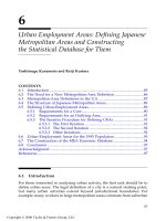
The magnitudes of agglomeration economies may also be different
between different size groups. Figure 16.1 shows estimates of the agglom-
eration economies coefficient

a

2

for three size groups: large MEAs with
300,000 or more employed workers, medium-sized MEAs with 100–300,000
workers, and small MEAs with less than 100,000 workers, in addition to the
coefficient for all MEAs. The coefficient is indeed larger for large MEAs,
while for small and medium-sized MEAs, the coefficient is negative.
In addition to the simultaneity problem, OLS cannot account for any
unobserved effects that represent any unmeasured heterogeneity that is cor-

FIGURE 16.1

Movement of agglomeration economies coefficient

a

2

: 1980–95.
–0.15
–0.10
–0.05
0.00
0.05
0.10
80 81 82 83 84 85 86 87 88 89 90 91 92 93 94 95
All MEAs Small MEAs Medium-sized MEAs Large MEAs

2713_C016.fm Page 233 Friday, September 2, 2005 8:26 AM

Copyright © 2006 Taylor & Francis Group, LLC

234

GIS-based Studies in the Humanities and Social Sciences

related with at least some of the explanatory variables. For example, the
climatic conditions of a city that affect its aggregate productivity may be
correlated with the number of workers because it influences their locational
decisions. These unobserved effects also bias the OLS estimates. To improve
these estimates, panel-data estimation with instrumental variables is used
to eliminate biases caused by the simultaneity problem and any unobserved
city-specific effects.

16.4 Panel Estimates

We first estimate the panel model whose error terms are composed of the
city-specific, time-invariant term,

c

i

, and the error term, u
it
, that varies over
both city i and time t,
(16.4)
where and d
t

is the time dummy. The use of the time dummy is equivalent to assuming
fixed, time-specific effects. Table 16.2 shows fixed- and random-effects esti-
mates. A random-effect model (RE) assumes the individual effects c
i
are uncor-
related with all explanatory variables, while a fixed-effect model (FE) does not
require the assumption. Though Hausman test statistics indicate the violation
of the random-effect assumption for medium-sized MEAs and all MEAs, the
estimation results of the random-effect model are more reasonable than those
of fixed effects (see Wooldridge, 2002, Chapter 10, for Hausman test statistics).
TABLE 16.2
Panel Estimates
All MEAs Small MEAs Medium MEAs Large MEAs
FE RE FE RE FE RE FE RE
a
1
0.279
***
0.310
***
0.354
***
0.376
***
0.281
***
0.325
***
0.170
***

0.194
***
(0.015) (0.014) (0.030) (0.027) (0.021) (0.020) (0.029) (0.026)
a
2
0.101
***
0.031
***
–0.016 –0.044 0.416
***
0.096
***
–0.044 0.059
***
(0.023) (0.007) (0.037) (0.030) (0.040) (0.026) (0.058) (0.010)
a
3
–0.084
***
–0.108
***
–0.147
***
–0.132
***
0.145
***
–0.061
*

–0.151
***
–0.113
***
(0.020) (0.017) (0.034) (0.029) (0.040) (0.031) (0.030) (0.026)
0.623 0.770 0.741 0.761 0.311 0.721 0.502 0.862
Hausman 39.6 11.3 132.5 21.3
Chi (5 percent) 28.9 28.9 28.9 28.9
Sample size 1888 528 896 464
Note: Numbers in parentheses are standard errors.
***
significant at 1 percent level;
*
significant
at 10 percent level.
yAakanagbdcu
it it it it t t i it
=+ + + + ++
01 2 3
yYN
it it it
= ln( / ), kKN
it it it
= ln( / ),
nN
it it
= ln( ),
gGN
it it it
= ln( / ),

R
2
2713_C016.fm Page 234 Friday, September 2, 2005 8:26 AM
Copyright © 2006 Taylor & Francis Group, LLC
Estimating Urban Agglomeration 235
The random-effect estimates of the agglomeration coefficient a
2
are about
5 percent and 9 percent for large and medium-sized groups, but negative
for small MEAs. Those for social-overhead capital are significantly negative
for all groups.
The estimation results in Table 16.2 fail to eliminate the simultaneity bias,
because both fixed- and random-effects models can deal only with the endo-
geneity problem stemming from the unobserved city-specific effects, c
i
. Cor-
relation between the random term, u
it
, and social-overhead capital still
provides a downward bias to the coefficients of social-overhead capital, and
the results presented in Table 16.2 may reflect this problem. These consider-
ations lead us to adopt a two-step GMM estimator, which, in this case, yields
the 3SLS estimation in Wooldridge (2002, chap. 8, p. 194–8). (See Wooldridge,
2002, Chapter 8, pp. 188–199, and Baltagi, 2001, Chapter 8, for the explanation
of GMM.)
We use time-variant instrumental variables (time dummies, k, n, and
squares of n) and time-invariant ones (average snowfall days per year for
the 30-year period 1971 to 2000 and their squares, and the logarithms of the
number of preschool children and the number of employed workers who
are university graduates in 1980). A major source of the bias could be the

tendency of u
it
to be negatively correlated with the social-overhead capital.
Appropriate instruments are then those that are correlated with the social-
overhead capital but do not shift the production function. The snowfall days
per year satisfy the first property, because additional social-overhead invest-
ment is often necessary in regions with heavy snowfalls. It is not clear if the
variable satisfies the second condition, since the inconvenience caused by
snow may also reduce productivity. The logarithms of the numbers of pre-
school children and employed workers who are university graduates in 1980
are correlated with the regional-income level that negatively influences the
interregional allocation of social-overhead capital. Since we use only the first
year of our data set, they are exogenous for the subsequent production
function, and it is reasonable to assume orthogonality with future idiosyn-
cratic errors.
The revised estimation results are presented in Table 6.3. The coefficients
of social-overhead capital are now positive but insignificant. The apparent
simultaneity bias for social-overhead capital is only partially eliminated.
Sargan’s J and F values from the first regression, shown in Table 16.3, test
the orthogonality condition for instrumental variables and the intensity of
correlation between instruments and endogenous variables to be controlled
(see Hayashi, 2000, Chapter 3, for Sargan’s J statistics). While the F statistics
are significant for all groups, the J statistics are significantly high for the two
cases of all MEAs and medium-sized MEAs. The former results imply that
the instruments we employed worked significantly well to predict the values
of endogenous variables in the first regression. The latter results imply,
however, that our instruments have failed to eliminate the simultaneity bias,
at least in the two cases. The source of the bias is then likely to be the
correlation between the instruments and city-specific, unobserved effects.
2713_C016.fm Page 235 Friday, September 2, 2005 8:26 AM

Copyright © 2006 Taylor & Francis Group, LLC
236 GIS-based Studies in the Humanities and Social Sciences
One possible solution is to apply GMM estimation to time-differenced equa-
tions, as argued by Arellano and Bond (1991) and Blundell and Bond (1998).
Both of these methods were tried but failed to yield satisfactory results. One
cause of this failure is the fact that instruments that do not change over time
cannot be used in the estimation of time-differenced equations.
The estimates of the agglomeration-economy parameter, a
2
, are smallest
for small MEAs and become larger for larger MEAs. An important difference
from the OLS and RE estimates is that the sign of a
2
is positive even for small
MEAs, which was negative in the earlier estimations. Accordingly, although
our GMM 3SLS estimates display a number of shortcomings, they yield more
reasonable estimates than those we have obtained elsewhere. We use the
GMM 3SLS estimates as the relevant agglomeration-economy parameter in
the next section.
16.5 A Test for Optimal City Sizes
Any policy discussion in economics must start with identification of the
sources of market failure. In general, an optimally sized city balances urban
agglomeration economies with diseconomy forces, and the first task is to
check if these two forces involve significant market failure. On the side of
agglomeration economies, a variety of microfoundations are possible,
including Marshallian externality models (Duranton and Puga, 2003), new
economic geography (NEG) models (Ottaviano and Thisse, 2003), and a
reinterpretation of the nonmonocentric city models of Imai (1982) and Fujita
and Ogawa (1982), as presented by Kanemoto (1990). Although the latter
two do not include any technological externalities, the agglomeration econ-

omies that they produce involve similar forms of market failure. That is,
TABLE 16.3
GMM 3SLS Estimates
All MEAs
Small
MEAs Medium MEAs Large MEAs
a
1
0.518
***
0.601
***
0.479
***
0.344
***
(0.030) (0.066) (0.047) (0.048)
a
2
0.044
***
0.027 0.053
***
0.068
***
(0.005) (0.018) (0.013) (0.007)
a
3
0.047 0.077 0.023 0.056
(0.033) (0.081) (0.069) (0.045)

J-statistics (D.F.) 16.28 (4) 5.73 (4) 24.57 (4) 3.78 (4)
Chi (5 percent) 9.49 9.49 9.49 9.49
1st stage F-statistics 216.85 81.10 105.19 91.73
Sample size 1888 528 896 464
Note:
***
significant at 1 percent level.
2713_C016.fm Page 236 Friday, September 2, 2005 8:26 AM
Copyright © 2006 Taylor & Francis Group, LLC
Estimating Urban Agglomeration 237
urban agglomeration economies are external to each individual or firm, and
a subsidy to increase agglomeration may improve resource allocation. This
suggests that agglomeration economies are almost always accompanied by
significant market failure.
In addition to these problems, the determination of city size involves
market failure due to lumpiness in city formation. A city must be large
enough to enjoy benefits of agglomeration, but it is difficult to create instan-
taneously a new city of a sufficiently large size, due to the problems of land
assembly, constraints on the operation of large-scale land developers, and
the insufficient fiscal autonomy of local governments. If we have too few
cities, individual cities tend to be too large. In order to make individual cities
closer to the optimum, a new city must be added. It may, of course, also be
difficult to create a new city of a large enough size that can compete with
the existing cities.
These types of market failure are concerned with two different “margins.”
The first type represents divergence between the social and private benefits
of adding one extra person to a city, whereas the second type involves the
benefits of adding another city to the economy. In order to test the first aspect,
we have to estimate the sizes of external benefits and costs. To the authors’
knowledge, no empirical work of this type exists concerning Japan. The

Henry George Theorem can test the second aspect. According to this theo-
rem, the optimal city size is achieved when the dual (shadow) values for
agglomeration and deglomeration economies are equal. For example, the
agglomeration forces are externalities among firms in a city, and the deglom-
eration forces are the commuting costs of workers who work at the center
of the city, then the former is the Pigouvian subsidy associated with the
agglomeration externalities, and the latter is the total differential urban rent.
Using the estimates of agglomeration economies obtained in the preceding
section, we examine whether the cities in Japan (especially Tokyo) are too
large. Our approach of applying the Henry George Theorem to test this
hypothesis is basically the same as that in Kanemoto et al. (1996) and
Kanemoto and Saito (1998). As noted in the preceding section, we consider
two polar cases concerning the social-overhead capital. One is the case where
the social-overhead capital is a private good, and firms pay for it. In this
case, the total Pigouvian subsidy is TPS = a
2
Y, and the Henry George Theo-
rem implies TDR = TPS, where TDR is the total differential rent of a city.
The other case assumes that the social-overhead capital is a pure, public
good, and firms do not pay its cost. The total Pigouvian subsidy is then TPS
= (a
2
– a
3
)Y, and the Henry George Theorem is TDR – C(G) = TPS, where
C(G) is the cost of the social-overhead capital.
Unfortunately, a direct test of the Henry George Theorem is empirically
difficult, because good land-rent data is not readily available, and land prices
have to be relied upon instead. Importantly, the conversion of land prices
into land rents is bound to be inaccurate in Japan, where the price/rent ratio

is extremely high and has fluctuated enormously in recent years. Roughly
speaking, the relationship between land price and land rent is: Land Price
2713_C016.fm Page 237 Friday, September 2, 2005 8:26 AM
Copyright © 2006 Taylor & Francis Group, LLC
238 GIS-based Studies in the Humanities and Social Sciences
= Land Rent / (Interest Rate – Rate of Increase of Land Rent. In a rapidly
growing economy, the denominator tends to be very small, and a small
change in land rents generally results in a large change in land prices, as
well as highly variable prices. For instance, the total real-land value of Japan
tripled from 600 trillion yen in 1980 to about 1800 trillion yen in 1990, and
then fell to some 1000 trillion yen in 2000. Given these possibly inflated and
fluctuating land-price estimates and the inability to get good land-rent data,
instead of testing the Henry George Theorem directly, we compute the ratio
between the total land value and the total Pigouvian subsidy for each met-
ropolitan area, to see if there is a significant difference in the ratio between
cities at different levels of the urban hierarchy.
Our hypothesis is that cities form a hierarchical structure, where Tokyo is
the only city at the top (see, for instance, Kanemoto, 1980; and Kanemoto et
al., 1996). While equilibrium city sizes tend to be too large at each level of
the hierarchy, divergence from the optimal size may differ across levels of
hierarchy. At a low level of hierarchy, the divergence tends to be small,
because it is relatively easy to add a new city. For example, moving the
headquarters or a factory of a large corporation can easily result in a city of
20,000 people. In fact, the Tsukuba science city, created by moving national
research laboratories and a university to a greenfields location, resulted in
a population of more than 500,000. However, at a higher level, it becomes
more difficult to create a new city, because larger agglomerations are gener-
ally more difficult to form. For example, the population-size difference
between Osaka and Tokyo is close to 20,000,000, and making Osaka into
another center of Japan would be arguably very difficult. We therefore test

whether the divergence from the optimum is larger for larger cities, in
particular if the ratio between the total land value (minus the value of the
social-overhead capital when it is a pure, public good) and the total Pigou-
vian subsidy is significantly larger for Tokyo than for other cities.
The construction of the total land-value data for an MEA is as follows.
The Annual Report on National Accounts contains the data on the value of
land by prefecture. We allocate this prefecture data to MEAs, using the
number of employed workers by place of residence. The first-round estimate
is obtained by simple, proportional allotment. The problem with this esti-
mate is that land value per worker is the same within a prefecture, regardless
of city size. In order to incorporate the tendency that it is larger in a large
city, we regress the total land value on city size, and use the estimated
equation to modify the land-value estimates. The equation we estimate is:
In (V
i
) = a ln(N
i
) + b where V
i
is the first-round estimate of the total land
value, N
i
is the number of employed workers in a MEA, and a and b are
estimated parameters. In the estimation, care has to be taken with sample
choice, because in Japan, there are many small cities and very few large
cities. If we include all MEAs, then the estimated parameters are influenced
mostly by small cities. Since we are interested in the largest cities, we include
the 19 largest MEAs in our sample. We drop the 20th largest MEA (Himeji),
because it belongs to the same prefecture as the much larger Kobe, and the
2713_C016.fm Page 238 Friday, September 2, 2005 8:26 AM

Copyright © 2006 Taylor & Francis Group, LLC
Estimating Urban Agglomeration 239
first-round estimate could then be seriously biased. The estimate of a is 1.20,
with t-value 21.45. Assuming , we compute the total land value of
an MEA by
. (16.5)
Table 16.4 presents the total land value, the total Pigouvian subsidy, and
social-overhead capital in the largest 20 MEAs in those cases where the
production-function parameters are given by the GMM estimate for large
MEAs in Table 16.3. The columns of “Pigouvian subsidy 1” and “Pigouvian
subsidy 2” show the subsidies in the first case, TPS = a
2
Y, and the second
case, TPS = (a
2
– a
3
)Y, respectively. In both cases, the two largest MEAs, Tokyo
and Osaka, have a significantly higher land value/Pigouvian subsidy ratio
than the average city. This result supports the hypothesis that Tokyo is too
large, but then it is likely that Osaka is also too large. These ratios are
computed for the remaining years, and the same tendency exists. These
results contrast with Kanemoto et al. (1996), who found that the land value/
Pigouvian subsidy ratio for Tokyo was slightly below the average for Japan’s
TABLE 16.4
Total Land Values and Pigouvian Subsidies
MEA Population
Land
Value (a)
Pigouvian

Subsidy 1
(b) (a)/(b)
Social-
Overhead
Capital (c)
Pigouvian
Subsidy 2
(d)
(a) – (c)/
(d)
Tokyo 30,938,445 518,810 9,493 55 133,310 1,613 239
Osaka 12,007,663 176,168 3,216 55 53,654 546 224
Nagoya 5,213,519 62,517 1,594 39 20,774 271 154
Kyoto 2,539,639 27,851 637 44 10.075 108 164
Kobe 2,218,986 21,913 575 38 12,345 98 98
Fukuoka 2,208,245 19,810 532 37 8,890 90 121
Sapporo 2,162,000 12,645 508 25 14,670 86 –23
Hiroshima 1,562,695 14,708 421 35 8,481 72 87
Sendai 1,492,610 12,529 377 33 7,604 64 77
Kitakyushu 1,428,266 11,059 311 36 6,719 53 82
Shizuoka 1,002,032 12,740 258 49 3,715 44 206
Kumamoto 982,326 6,505 206 32 4,892 35 46
Okayama 940,208 7,637 230 33 5,370 39 58
Niigata 936,750 7,519 231 33 5,698 39 46
Hamamatsu 912,642 11,489 242 47 3,707 41 189
Utsunomiya 859,178 8,021 223 36 3,551 38 118
Gifu 818,302 6,709 187 36 3,800 32 92
Himeji 741,089 6,143 205 30 4,640 35 43
Fukuyama 729,472 5,367 174 31 4,433 29 32
Kanazawa 723,866 7,412 182 41 3,957 31 112

Average 47,878 990 38 16,014 168 108
Note: Land value, Pigouvian subsidy, and social-overhead capital are in billion yen.
VAN
ii
a
=
V
V
N
N
i
j
a
i
a
=
∑
2713_C016.fm Page 239 Friday, September 2, 2005 8:26 AM
Copyright © 2006 Taylor & Francis Group, LLC
240 GIS-based Studies in the Humanities and Social Sciences
largest 17 metropolitan areas. One possible source of this difference is the
land-value estimates used in this study, since the land values of Tokyo and
Osaka are generally much higher than those in other Japanese cities.
Outside of Tokyo and Osaka, Shizuoka, Hamamatsu, and Kyoto also have
high land value/Pigouvian subsidy ratios. This pattern is the same in the
pure, public-good case. In the pure, public-good case, Sapporo has a negative
ratio, because the value of social-overhead capital exceeds the total land
value. This is caused by the fact that Sapporo is located on Hokkaido Island,
and therefore receives a disproportionately high share of social-overhead
capital investment.

16.6 Conclusion
Using the estimates of the magnitudes of agglomeration economies derived
from aggregate production functions for metropolitan areas in Japan, we
have examined the hypothesis that Tokyo is too large. In a simple, cross-
section estimation of a metropolitan production function, the coefficient for
social-overhead capital is either negative or statistically insignificant. The
main reason for this is a simultaneity bias arising from social-overhead
capital being more heavily allocated to low-income regions in Japan. In order
to correct for this bias, we adopted panel-data methods. Simple fixed-effects
and random-effects estimators still yield negative estimates. We also intro-
duced instrumental variables and applied the GMM 3SLS to our panel data.
The estimates become positive, but insignificant. The instrumental variables
appear to reduce such bias, but they may not be strong enough to yield an
unbiased estimate.
Using the GMM estimates for agglomeration economies, we also examined
whether the Henry George Theorem for optimal city size is satisfied. Tokyo
and Osaka have a higher land value/Pigouvian subsidy ratio than other
cities. This indicates that Tokyo and Osaka are too large on the basis of this
criterion. However, these results are tentative, and elaboration and extension
in many different directions may be necessary.
Acknowledgment
This research is supported by the Grants-in-aid for Scientific Research
No.10202202 and No. 1661002 of the Ministry of Education, Culture, Sports,
Science and Technology.
2713_C016.fm Page 240 Friday, September 2, 2005 8:26 AM
Copyright © 2006 Taylor & Francis Group, LLC
Estimating Urban Agglomeration 241
References
Abdel-Rahman, H. and Fujita, M., Product variety, Marshallian externalities, and city
sizes, J. Reg. Sci., 30, 165–183, 1990.

Arellano, M. and Bond, S., Some tests of specification for panel data: Monte Carlo
evidence and an application to employment equations, Rev. Econ. Stud., 58,
277–297, 1991.
Baltagi, B.H., Econometric Analysis of Panel Data, 2nd ed., John Wiley & Sons, Chich-
ester, 2001.
Blundell, R. and Bond, S., Initial conditions and moment restrictions in dynamic
panel data models, J. Econ., 87, 115–143, 1998.
Duranton, G. and Puga, D., Micro-foundations of urban agglomeration economies,
in Handbook of Urban and Regional Economics, Vol. 4, Henderson, J.V. and Thisse,
J F., Eds., North-Holland, Amsterdam, 2063–2117, 2004.
Hayashi, F., Econometrics, Princeton University Press, Princeton, New Jersey, 2000.
Iwamoto, Y., Ouchi, S., Takeshita, S., and Bessho, T., Shakai Shihon no Seisansei to
Kokyo Toshi no Chiikikan Haibun (Productivity of social overhead capital and
the regional allocation of public investment), Financ. Rev., 41, 27–52, 1996 (in
Japanese).
Kanemoto, Y., Theories of Urban Externalities, North-Holland, Amsterdam, 1980.
Kanemoto, Y., Optimal cities with indivisibility in production and interactions be-
tween firms, J. Urb. Econ., 27, 46–59, 1990.
Kanemoto, Y., Ohkawara, T., and Suzuki, T., Agglomeration economies and a test for
optimal city sizes in Japan, J. Jpn. Int. Econ., 10, 379–398, 1996.
Kanemoto, Y. and Saito, H., Tokyo wa Kadai ka: Henry George Teiri ni Yoru Kensho
(Is Tokyo too large? A test of the Henry George Theorem), Hous. Land Econ.
(Jutaku Tochi Keizai), 29, 9–17, 1998 (in Japanese).
Ottaviano, G. and Thisse, J F., Agglomeration and economic geography, in Handbook
of Urban and Regional Economics, Vol. 4, Henderson, J.V. and Thisse, J F., Eds.,
North-Holland, Amsterdam, 2564–2608, 2004.
Wooldridge, J.M., Econometric Analysis of Cross Section and Panel Data,: MIT Press,
Cambridge, Massachusetts, 2002.
2713_C016.fm Page 241 Friday, September 2, 2005 8:26 AM
Copyright © 2006 Taylor & Francis Group, LLC