Regional Scale Ecological Risk Assessment - Chapter 2 potx

11

C

HAPTER

2
Introduction to the Regional Risk
Assessment Using the Relative Risk Model

Wayne G. Landis and Janice K. Wiegers

CONTENTS

Introduction 12
Regional Risk Assessment Defined 12
Framework of the Relative Risk Model 13
The 10 Steps of the Relative Risk Model
for Regional Risk Assessment 15
Step 1. List the Important Management Goals for the Region.
What Do You Care about and Where? 18
Step 2. Make a Map. Include Potential Sources and Habitats Relevant
to the Management Goals 19
Step 3. Break the Map into Regions Based upon a Combination
of Management Goals, Sources, and Habitats 20
Step 4. Make a Conceptual Model that Ties the Stressors to the
Receptors and to the Assessment Endpoints 20
Step 5. Decide on a Ranking Scheme for Each Source, Stressor, and
Habitat to Allow the Calculation of Relative Risk to the Assessment
Endpoints 22

Step 6. Calculate the Relative Risks 23
Integrating Ranks and Filters 23
Step 7. Evaluate Uncertainty and Sensitivity Analysis
of the Relative Rankings 24
Step 8. Generate Testable Hypotheses for Future Field and Laboratory
Investigation to Reduce Uncertainties and to Confirm the Risk Rankings 26
Step 9. Test the Hypotheses Listed in Step 8 27

L1655_book.fm Page 11 Wednesday, September 22, 2004 10:18 AM
© 2005 by CRC Press LLC

12 REGIONAL SCALE ECOLOGICAL RISK ASSESSMENT

Step 10. Communicate the Results in a Fashion that Portrays the
Relative Risks and Uncertainty in a Response to the Management Goals 27
Overview of the Relative Risk Model Studies 28
References 34

INTRODUCTION

Since 1997 the relative risk model (RRM) proposed by Wiegers and Landis
(Landis and Wiegers 1997; Wiegers et al. 1998) has been used at a variety sites to
generate regional risk hypotheses on a variety of scales. These scales have ranged
from an urban watershed a few square kilometers in size, to a Brazilian rain forest,
and to coastal marine areas. The studies also incorporate multiple sources of multiple
stressors with a variety of endpoints that exhibit a spatial and temporal distribution.
The purpose of this chapter is to define regional risk assessment, present the RRM,
and to briefly summarize the scope and results of the studies conducted up until the
fall of 2003.

REGIONAL RISK ASSESSMENT DEFINED

Ecological risk assessment calculates the probability of an impact to a specified
set of assessment endpoints over a defined period of time. In the risk assessment of
chemicals, exposure and effects are estimated and the probability of the intersection
of those functions calculated. Impacts typically considered are mortality, chronic
physiological impacts, and reproductive effects. Most often these risk assessments
deal with single chemicals in such classic cases as pesticides, herbicides, organic
solvents, metals, polychlorinated biphenyls, and dioxins. Most often the risk assess-
ments dealt with only one or a few biological endpoints.
During the 1990s there was an effort to expand ecological risk assessment to
more accurately reflect the reality of the structure, function, and scale of ecological
structures. Hunsaker, O’Neill, Suter and colleagues (Hunsaker et al. 1990; Suter
1990; O’Neill et al. 1997) formulated the idea of performing regional risk assess-
ments at a landscape scale. There have been attempts to perform risk assessment
based upon the classical U.S. Environmental Protection Agency (USEPA) paradigm,
but each has had limitations (Cook et al. 1999; Cormier et al. 2000) imposed by a
risk assessment framework originally designed for single chemicals and receptors.
A principal difficulty is the incorporation of the spatial structure of the environment
and the inherent presence of multiple stressors.
We (Landis and Wiegers 1997; Wiegers et al. 1998) adopted a definition that
naturally incorporates multiple stressors, historical events, spatial structure, and
multiple endpoints. Our working definition of a regional-scale risk assessment is:

A risk assessment deals at a spatial scale that contains multiple habitats with multiple
sources of multiple stressors affecting multiple endpoints and the characteristics of
the landscape affect

the risk estimate. Although there may only be one stressor of
concern, at a regional scale the other stressors acting upon the assessment endpoints
are to be considered.

L1655_book.fm Page 12 Wednesday, September 22, 2004 10:18 AM
© 2005 by CRC Press LLC

INTRODUCTION TO THE REGIONAL RISK ASSESSMENT 13

FRAMEWORK OF THE RELATIVE RISK MODEL

The framework for the RRM for regional risk assessment was outlined by Landis
and Wiegers (1997). Ecological risk assessment (EcoRA) methods traditionally
evaluate the interaction of three environmental components: stressors released into
the environment, receptors living in and using that environment, and the receptor
response to the stressors (Figure 2.1a). Measurements or estimates of exposure and
effect quantify the degree of interaction between these components. At a single
contaminated site, especially where only one stressor is involved, the connection of
the exposure and effect measurements to the assessment endpoints can be relatively
simple. However, in a regional multiple stressor assessment, the number of possible
interactions increases dramatically. Stressors arise from diverse sources, receptors
are often associated with a variety of habitats, and one impact may lead to additional
impacts. A complex background of sets of natural stressors and effects further clouds
the picture.
Expanding an assessment to cover a region requires consideration of larger-scale
regional components: sources that release multiple stressors, habitats where the
multiple receptors live, and the multiple impacts to the assessment endpoints (Figure
2.1b). The three regional components are analogous to the three traditional compo-
nents, but the emphasis is on location and groups of stressors, receptors, and effects.
Traditional risk assessment estimates the level of exposure and effect to calculate

risk. However, exposure and effect cannot be directly measured unless a specific
stressor and a specific receptor are identified. At a regional level, stressors and
receptors can be represented as groups: a source as a group of stressors, a habitat
as a group of receptors, and an ecological impact as a group of receptor responses.
These combinations involve the use of a variety of distinctly different measurements.

Figure 2.1

Comparison of traditional risk assessment to regional relative risk assessment.
STRESSOR
RECEPTOR
RESPONSE
measured/
estimated
exposure effect
measured/
estimated
SOURCES of
STRESSORS
HABITATS
ECOLOGICAL
IMPACTS
RANKED
ranked
exposures
ranked
effects
Locations of Multiple
Stressors
Locations of Multiple

Receptors
Locations of Multiple
Responses
Filter
Filter
(a) Traditional Risk Assessment Components
(b)

Regional Relative Risk Assessment Components

L1655_book.fm Page 13 Wednesday, September 22, 2004 10:18 AM
© 2005 by CRC Press LLC

14 REGIONAL SCALE ECOLOGICAL RISK ASSESSMENT

For example, the measurement of a polychlorinated organic compound will results
in units, mg/L, distinctly different from the occurrence of an invasive species, number
of organisms/m

2

. Yet both can be present within the area of study. Impacts can be
similarly varied, mortality may have to be combined with a decrease with the
occurrence of nonindigenous species

.

It is very intractable to attempt to combine
measurements taken with distinctly different units.
However, it is possible to combine these measurements based on the establish-

ment of ranks. In this manner a concentration of a chemical that may cause a high
degree of mortality can be combined with an invasion of a new species that will
alter a small amount of habitat. The criteria for setting ranks are discussed later, but
the crucial feature is that this approach allows the evaluation of multiple stressors
being derived from multiple sources impacting a variety of species in a variety of
habitats in a variety of locations.
Relative regional assessment identifies the sources and habitats in different
locations of the site, ranks their importance in each location, and combines this
information to predict relative levels of risk. The number of possible risk combina-
tions resulting from this approach depends on the number of categories identified
for each regional component. For example, if two source types (e.g., point discharge
and fish waste) and two habitat types (e.g., the benthic environment and the water
column) are identified, then four possible combinations of these components can
lead to an impact. If in addition we are concerned about two different impacts (e.g.,
a decline in the sport fish population and a decline in sediment quality), eight possible
combinations exist.
Each identified combination establishes a possible pathway to a risk in the
environment. If a particular combination of components interacts or affects another,
then they can be thought of as overlapping. When a source generates stressors that
affect habitats important to the assessment endpoints, the ecological risk is high. A
minimal interaction between components results in a low risk. If one component
does not interact with one of the other two components, no risk exists. For example,
a discharge piped into a deep water body is not likely to impact salmon eggs, which
are found in streams and intertidal areas. In such a case, the source component (an
effluent discharge) does not interact with the habitat (streams and intertidal areas),
and no impact would be expected (i.e., harm to the salmon eggs). This is analogous
to the overlap among the stressor, receptor, and hazard in conventional risk assess-
ment. Impact 1 may also be due to the overlap of several sources of stressors with
several habitats, all altering the risk. Integrating these combinations demonstrates
that impact 1 is actually the result of several combinations of sources and habitats.

To fully describe the risk of a single impact occurring, each possible route to the
impact needs investigation.
Integration of these routes is not always a simple matter and is again facilitated
by the use of ranks. Often, measurements of various exposure and effect levels
cannot be added together to determine the overall impact to the assessment endpoint.
For example, a decline in wild salmon populations can result from a combination
of eggs in the spawning grounds being exposed to chemicals and increased predation
when the juveniles migrate out of the port. However, chemical exposure to the eggs
may also influence growth of the juvenile fish. Smaller fish are less able to avoid

L1655_book.fm Page 14 Wednesday, September 22, 2004 10:18 AM
© 2005 by CRC Press LLC

INTRODUCTION TO THE REGIONAL RISK ASSESSMENT 15

predation, and mortality from predation may increase beyond what would be
expected if the effect to the eggs was not considered.
The RRM regional approach is a system of numerical ranks and weighting factors
to address the difficulties encountered when attempting to combine different kinds
of risks. Ranks and weighting factors are unitless measures that operate under

2

measurements exist that are additive. For example, there is little meaning in adding
toxicant concentrations to counts of the number of introduced predators in order to
determine the total risk in a system. However, knowing that a particular region has
both the highest concentrations of a contaminant and the most introduced predators
is useful in a decision-making process.
The next sections take this basic approach and describe the steps in conducting
a regional relative risk assessment, from problem formulation to risk communication.

THE 10 STEPS OF THE RELATIVE RISK MODEL
FOR REGIONAL RISK ASSESSMENT

The previous reviews of the application of the RRM have led to the formulation
of ten procedural steps that formalize the process. The process can also generate
three specific outputs useful in the decision-making process.
The procedural steps are

1. List the important management goals for the region. What do you care about and
where?
2. Make a map. Include potential sources and habitats relevant to the management
goals.
3. Break the map into regions based upon a combination of management goals,
sources, and habitats.
4. Make a conceptual model that links sources of stressors to the receptors and to
the assessment endpoints.
5. Decide on a ranking scheme to allow the calculation of relative risk to the
assessment endpoints.
6. Calculate the relative risks.
7. Evaluate uncertainty and sensitivity analysis of the relative rankings.
8. Generate testable hypotheses for future field and laboratory investigation to reduce
uncertainties and to confirm the risk rankings.
9. Test the hypotheses listed in Step 8.
10. Communicate the results in a fashion that portrays the relative risks and uncertainty
in a response to the management goals.

These ten steps correspond to the portions of the ecological risk assessment
the initial segments of the framework, especially problem formulation. These initial
steps largely determine the success of the risk assessment. Steps 4, 5, and 6 are

closely related and do not fit cleanly into conventional framework. The conceptual

L1655_book.fm Page 15 Wednesday, September 22, 2004 10:18 AM
© 2005 by CRC Press LLC
different limitations than measurements with units (e.g., mg/L, individuals/cm ) (Figure
2.2). In a complex system with a wide range of dissimilar stressors and effects, few
framework as depicted in Figure 2.3. The first four steps of the RRM correspond to

16 REGIONAL SCALE ECOLOGICAL RISK ASSESSMENT

Figure 2.2

The application of ranks and filters in the RRM scheme.
high discharge or activity
from the source in the
subarea
low discharge or activity
from the source in the
subarea
no sources of this type
in the area
4
Source Type
Habitat Type
large amount of the
habitat in the subarea
moderate discharge or
activity from the source
in the subarea
moderate amount of the

habitat type in the sub-
area
small amount of the
habitat type in the sub-
area
no habitats of this type
in the area
Rank
6
2
0
A
0
source
habitat
the source is
unlikely
to occur
or be transported into the habitat
1
Scalar
Exposure Combination
the source is
likely
to occur
or be transported into the habitat
source habitat
B
0
the impact is

unlikely
to occur in the
habitat or because of the source
1
Scalar
Effect Combination
source habitat
source
habitat
the impact is
likely
to occur in the


habitat or because of the source
impact
impact
C
SOURCE
HABITAT
ECOLOGICAL
IMPACT
Sum of ranks for
each possible
combination of
sources and habitats

L1655_book.fm Page 16 Wednesday, September 22, 2004 10:18 AM
© 2005 by CRC Press LLC
© 2005 by CRC Press LLC

INTRODUCTION TO THE REGIONAL RISK ASSESSMENT 17

model is based upon knowledge of source–stressor–habitat–effects linkages. Deter-
mination of the ranking scheme incorporates a large quantity of data generated on
the amounts of stressors, habitats, and what knowledge is available on potential
outcomes. Once the conceptual model and ranking scheme are established the actual
calculation is straightforward. Analysis of uncertainty and sensitivity and generation
of testable hypotheses are the more difficult steps that most closely correspond to
risk characterization. Testing the hypotheses corresponds to the verification step and
should be incorporated whenever possible.
Step 10 corresponds to risk communication and is comprised of three outputs.

1. Maps of the risk regions with the associated sources, landuses, habitats, and the
spatial distribution of the assessment endpoints.
2. A regional comparison of the relative risks, their causes, the patterns of impacts
to the assessment endpoints, and the associated uncertainty. These regional com-
parisons and estimates of the contribution of each source and stressor create a
spatially explicit risk hypothesis.
3. A model of source–habitat–impact that can be used to ask what-if questions about
different scenarios that are potential options in environmental management.

These outputs summarize the data and provide risk assessments and a tool for
the examination of different risk scenarios. These outputs facilitate communication
and decision making for the environmental managers. The next section describes
each of the ten steps and the three outputs.

Figure 2.3

Relationship of the ten steps in the RRM to the classic ecological risk assessment

paradigm.
Problem
Formulation
Risk
Characterization
Risk
Communication
Analysis
1,2,3,4
5
6,7,8,9
10
Ten Steps
Ecological Risk
Assessment Framework
Verification
Decision
Maker

L1655_book.fm Page 17 Wednesday, September 22, 2004 10:18 AM
© 2005 by CRC Press LLC

18 REGIONAL SCALE ECOLOGICAL RISK ASSESSMENT

The first four steps are critical to performing a regional ecological risk assessment
and are the foundation of a useful risk assessment that can be applied to the decision-
making process and to long-term environmental management. These steps should
involve close interaction with all of the interested parties. The parties include the
regulators, the regulated community, the stakeholders comprised of private citizens
and nongovernmental organizations, and the risk assessors. There are likely to be

environmental managers in the first three groups who will be involved in the decision-
making process. The risk assessors need to clearly understand the decision-making
needs of each of the other groups, communicate the strengths and limitations of the
risk assessment process, and attempt to translate management goals stated in non-
scientific terminology to features that can be quantified and evaluated. In this inter-
action the role of the risk assessor is clearly not decision making, but scientific and
technical support. At times the decision makers may need to know that a particular
goal is not part of ecological reality, or that the field of science is not sufficiently
advanced to provide predictive measures. However, the interaction is critical if a
successful risk assessment is to occur.

Step 1. List the Important Management Goals for the Region.
What Do You Care about and Where?

The management goals are the key to the rest of the risk assessment. Regional
risk assessments are most effective when they target the decision-making needs and
goals of environmental managers. It is important to identify difficult or even con-
flicting goals. Decisions must be identified early in the process. Without identifying,
discussing, and resolving these issues, the assessment results will not appear to be
useful to managers, and in fact may not be usable for the decisions at hand.
There are four sets of interactions among the regulated community, the regula-
tors, and the interested stakeholders in the decision-making process. Interaction
among these three groups is expected in three forms. First, each will interact with
the other two parties in a bipartite fashion. Second, all three parties must interact at
the same time to clearly define the management and decision options in order to
answer basic questions about the future management of the area. Third, there are
also interactions between the three groups and the risk assessment team.
The role of the risk assessment team is critical. In some instances the desired
uncertainty reduction is not possible due to resource limitations (Suter 1993), and
some management goals are unattainable as well. While a goal may be to restore

the balance of nature or to return the system to a pristine state, given our current
understanding of ecological systems, neither of these goals is attainable (Landis and
McLaughlin 2000

)

. However, stakeholders envision the restoration of certain eco-
logical resources to within usable limits, and these goals can be quantified and
engineered.
The management goals for the fjord of Port Valdez and the Codorus Creek
watershed in Pennsylvania were derived from public meetings with representatives
of the various stakeholder groups. These groups included the regulated community,
the regulators, interested stakeholders, and the risk assessors.

L1655_book.fm Page 18 Wednesday, September 22, 2004 10:18 AM
© 2005 by CRC Press LLC

INTRODUCTION TO THE REGIONAL RISK ASSESSMENT 19

In some instances, such as the Willamette–McKenzie risk assessment, a similar
process may already have been performed by the appropriate stakeholder groups.
In the Willamette–McKenzie study the values were derived from the Willamette
Valley Livability Forum, a group established by the governor of Oregon with a
charge of establishing management goals for the ecological services provided by
the Willamette River and its tributaries. The process was driven by consensus for
the period up to 2050. The management goals for fisheries are shown in Table 2.1

.

The first column lists the goals as defined by this group. The second column is the

quantitative measure that we used to define this goal. In some areas there are conflicts
where two desired goals appear incompatible, but the goal of the risk assessment
team is to be as inclusive as possible.
As this process is completed the management goals are then placed into a spatial
context with the appropriate sources and habitats.

Step 2. Make a Map. Include Potential Sources and Habitats Relevant
to the Management Goals

As an example we will use the map-making process for the Cherry Point study,
but all of the studies to date incorporate a similar process. First, the potential sources
within the study area are located, characterized, and placed on a map that includes
the critical topological features of the system. The boundaries are set by the man-
agement goals of the decision makers, but also take into account the life history of
the various endpoints. Habitat information is also plotted for the endpoints under
consideration. Maps can be produced in a variety of ways; the Port Valdez study
utilized conventional maps scanned into a computer and the additional information
was added in a graphics program. Subsequent studies have made extensive use of
geographical information systems (GIS) that have distinct advantages and disadvan-
tages. The advantages are clearly the ability to display and analyze geographical

Table 2.1 Examples of Stakeholder Values for Two Sites of Regional-Scale

Risk Assessments
Willamette–McKenzie River, OR Codorus Creek, PA

River water is usable as source of drinking
water
Fish from river are palatable and safe to eat
There are sufficient numbers of desirable fish

to support an active recreational and
commercial fishery
Summer steelhead populations
Spring chinook salmon populations
River sustains thriving populations of native fish
Floodplain protection and enhancement for
natural functions and values
Floodplain management for human health and
safety
Water quantities sustain human communities
Maintain reservoirs for fishing, boating, and
windsurfing
Protective water quality for aquatic ecological
receptors and humans during contact or
consumption
Adequate water supply for drinking and
waste discharge
Self-sustaining native and nonnative fish
populations in the watershed
Adequate food availability for aquatic species
Available recreational land and water
resources
Adequate stormwater control and treatment

L1655_book.fm Page 19 Wednesday, September 22, 2004 10:18 AM
© 2005 by CRC Press LLC

20 REGIONAL SCALE ECOLOGICAL RISK ASSESSMENT

information in a variety of formats. Unfortunately, not all spatial data are in digital

form, digital data can often be expensive when it does exist, and digital data are
kept in a variety of projections which take time to combine. Uncertainty related to
geographical information is also an issue that will be discussed in Step 7.
The next step is to combine management objectives, source information, and
habitat data into geographically explicit portions that can be analyzed in a relative
manner.

Step 3. Break the Map into Regions Based upon a Combination
of Management Goals, Sources, and Habitats

The next step is the creation of risk regions that delineate the boundaries of the
areas for which risks will be calculated. This map is the basis of the rest of the
analysis because risks are all relative based upon the delineated regions. The map
is also based upon possible pathways of exposure in a spatial sense to the locations
where habitat can be found for the assessment endpoints. In this regard it may be
very important to follow fate of the water, groundwater, soil, and air within the
landscape to ensure that appropriate sources, stressors, and habitats are incorporated
into a risk region. The chapters that follow in this text provide a variety of methods
of deriving risk regions.

Step 4. Make a Conceptual Model that Ties the Stressors to the
Receptors and to the Assessment Endpoints

The conceptual model delineates the potential connections between sources,
stressors, habitat, and endpoints that will be used in each risk region. An example
of such a conceptual model for hypothetical regional-scale mining and smelting site

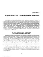
heavily forested area along a major river, with dams, transportation corridors, and
other activities occurring in the same region. The conceptual model is an extension of
the basic framework for a regional risk assessment with sources providing stressors

into particular habitats. In this instance the habitats are broadly defined as terrestrial
and aquatic to capture the exposure pathways and location within the region of our
endpoints. There are numerous interconnected endpoints both to show the valued
ecosystem components and to illustrate the interdependence and potential indirect
effects.
In cases (such as this illustration) where metals can be assumed to be the principal
contaminant, it is important to incorporate all of the confounding stressors. The
shaded boxes (Figure 2.4) highlight the conceptual model if only metals were being
considered. However, all of the endpoints are also being impacted by other stressors
as well. A metals-only assessment would take the endpoints and the metals out of
context.
A well-constructed and informative conceptual model places the site, the stres-
sors, the habitats, and the effects into a regional context. Such a construction can
eliminate some stressors due to the lack of exposure pathways and lead to the
inclusion of confounding factors outside the original scope of the assessment.

L1655_book.fm Page 20 Wednesday, September 22, 2004 10:18 AM
© 2005 by CRC Press LLC
is presented in Figure 2.4 and was constructed by E. Hart Hayes. The site is in a

INTRODUCTION TO THE REGIONAL RISK ASSESSMENT 21

Figure 2.4

Example of a conceptual model incorporating the basic framework of the relative risk model (designed by Hart Hayes). (See color
Sources
Stressors
Endpoints
Terrestrial Plants
Herbivorous Wildlife/

Animals
-South Red-backed Voles
-Columbia Ground Squirrel
-Horse
-Cow
-Chicken
Omnivorous Wildlife
Carnivorous Wildlife
Piscivorous Wildlife
Disturbance to Wildlife
Fragmentation of Terrestrial Habitat
Increased
Surface Runoff
-Erosion
-Sedimentation
Change Water Temperature
Blockage to Fish
Surface Water
Ground Water
Soil
Air
Soil
Macroinvertebrates
-Air Emissions
-Water Emissions
-Stack, Effluent & Fugitive
Sources
-Railway
-Roads
-Utility Corridors

-Forest Roads
-Clearcuts
Key
Chemicals
Stressors from Dam
Fragmentation of Habitat
Increased Runoff/Erosion/
Sedimentation
Disturbance to Wildlife
Aquatic Plants

Fish
Habitats
Smelter
Dam
Transportation
Pulp Mill
Forestry
Residential Landuse
Agricultural Landuse
Recreation
Ski Areas
Aquatic
Macroinvertebrates
-Black Bear
-Black-capped Chickadee
-Deer Mouse
-Red Squirrel
-American Crow
-Coyote

-Dusky Shrew
-Red-tailed Hawk
-American Robin
-Osprey
-River Otter
-Belted Kingfisher
Contaminants
-Chemicals of Concern
-Other (dioxins, PAHs, etc)

L1655_book.fm Page 21 Wednesday, September 22, 2004 10:18 AM
© 2005 by CRC Press LLC
insert following page 178.)

22 REGIONAL SCALE ECOLOGICAL RISK ASSESSMENT

Step 5. Decide on a Ranking Scheme for Each Source, Stressor, and
Habitat to Allow the Calculation of Relative Risk to the
Assessment Endpoints

This step changes data into nondimensional ranks so that effects due to the
various stressors to the various endpoints can be compared (Table 2.2). Each source
and habitat is ranked between subareas to indicate whether it is high, moderate, or
low within the context of the region. Ranks are assigned using criteria specific to
the study region. The criteria are based typically on the size and frequency of the
source and the amount of available habitat. Ranks are assigned for each source and
habitat type, generally on a two-point scale from 0 to 6 where 0 indicates no habitat
or source and 6 is the greatest amount.
There are different means of determining the criteria for ranks. In some instances
there may be adequate concentration response and fate of the stressor data available

to assign ranks to a particular source. For an effluent containing one nonpersistent
compound, below an EC10 could be zero, EC10 to EC30 could be low, EC30 to
EC50 medium, and greater than an EC50 could be high. Typically, that type of data
is not available for most stressors arising from a source.
In the chapters that follow there are many examples of ranking schemes with
the criteria listed in the accompanying tables. In the case of the Port Valdez scenario
to show all the variables included in the risk assessment. In some instances clustering
algorithms (Codorus Creek, Squalicum Creek, Cherry Point, etc.) were used to
determine natural breaks for the ranking criteria. The details are presented in the
following chapters.

Table 2.2

Example of Ranking Criteria for Stressors for Codorus Creek, PA
Coverage Criteria Ranks Example — Risk Region 1 Rank Scores

Landuse

Industrial % Industrial
< 1
< 1–2
2–16
6 (high)
4 (medium)
2 (low)
< 1% Industrial = Rank of

2
Soil Erosion

Vegetation Crops
Forest
Grass
6 (medium)
4 (medium)
2 (low)
16% Crops, 59% Forest, 24% Grass
(0.16

×

6) + (0.59

×

4) + (0.24

×

2) =

3.5

Soils > 8% Slope
3–8% Slope
0–3% Slope
6 (high)
4 (medium)
2 (low)
70% Slope > 8%, 25% Slope 3–8%, 5%

Slope 0–3
(0.70

×

6) + (0.25

×

4) + (0.05

×

2) =

5.3

Average 4.4

Altered Channel Structure

Channelization Channelized
Not Channelized
6 (high)
0 (no impact)
Not Channelized =

0

L1655_book.fm Page 22 Wednesday, September 22, 2004 10:18 AM

© 2005 by CRC Press LLC
(Chapter 4) these tables have been expanded beyond those of the original publication

INTRODUCTION TO THE REGIONAL RISK ASSESSMENT 23

Step 6. Calculate the Relative Risks

Filters determine the relationships among the risk components (source, habitat,
and impact to assessment endpoints). A filter consists of the weighting factors, 0 or
1, that indicate either a low or a high probability. We have incorporated two types
of filters: an

exposure filter

and an

effect filter

. The exposure filter screens the source
and habitat types for the combinations most likely to result in exposures (i.e.,
receptors in the habitat will come into contact with stressors generated by the source).
The effect filter screens the source and habitat combinations for those most likely
to affect a specific assessment endpoint. The examples below describe the design
of both an exposure and an effects filter

.

The first step in designing an exposure filter is to determine which stressors are
produced by the sources. Professional knowledge is then used to answer two sequen-
tial questions about each stressor in relation to specific source–habitat combinations:

•Will the source release or cause the stressor?
•Will the stressor then occur and persist in the habitat?

If the answer to both questions is yes, then 1 is assigned to the source–habitat
combination. If the answer to either question is no, then 0 is assigned.
The design of an effect filter is similar, but a separate filter is made for each
assessment endpoint. The first step in this process is to determine what type of effects
is important to the specific endpoint. For instance, if maintaining crab populations
is an assessment endpoint, some of the important effects to consider are toxicity,
predation, and food availability. The questions asked to develop the effect filters are:

•Will the source release stressors known to cause this particular effect to the
endpoint?
• Are receptors associated with the endpoint sensitive to the stressor in this habitat?

If the answer to both questions is yes, then 1 is assigned to the source–habitat
combination. If the answer to either question is no, then 0 is assigned.

Integrating Ranks and Filters

Ranks and weighting factors are combined through multiplication. The results
are a relative estimate of risk in each subarea. Final risk scores (RS) are calculated
for each subarea by multiplying ranks by the appropriate weighting factor (W

ij

) as
indicated below.
RS = S

ij



×

H

ik



×

W

jk

(2.1)
where:
i = the subarea series (Region 1, 2, 3, etc.),
j = the source series (discharge …, shoreline activity),
k = the habitat series (mudflat …, stream mouth),

L1655_book.fm Page 23 Wednesday, September 22, 2004 10:18 AM
© 2005 by CRC Press LLC

24 REGIONAL SCALE ECOLOGICAL RISK ASSESSMENT

S

ij

= rank chosen for the sources between subareas,
H

ik

= rank chosen for the habitats between subareas,
W

jk

= weighting factor established by the exposure or effect filter.
The results form a matrix of risk scores related to the relative exposure or effects
associated with a source and habitat in each subarea. The potential risk resulting
from a specific source (Equation 2.2) and occurring within a specific habitat (Equa-
tion 2.3) can be summarized for each subarea by adding the related scores,
RS

source

=

∑

(S

ij

×

H

ik



×

W

jk

) for j = 1 to n, (2.2)
RS

habitat

=

∑

(S

ij

×

H

ik



×

W

jk

) for k = 1 to n. (2.3)

Step 7. Evaluate Uncertainty and Sensitivity Analysis
of the Relative Rankings

Uncertainty needs to be accounted for and tracked in the risk assessment process.
Narratives can list the factors that introduced uncertainty into the assessment process.
It is also possible to examine uncertainty in a variety of quantitative means including
the Monte Carlo process employed to provide a range of values.
In the case of the Codorus Creek risk assessment (Obery and Landis 2002), three
sensitivity evaluations were performed to examine uncertainty of the model. These
methods were single-component analysis, exposure pathway analysis, and random
component analysis. Single-component analysis consisted of standardizing individ-
ual stressors in each of the risk regions to test the sensitivity of the model. Exposure

pathway analysis consisted of altering pathways with weak relationships in the
conceptual model warranting inclusion or exclusion in the evaluation. This uncer-
tainty analysis was warranted because only pathways demonstrating a strong rela-
tionship between the stressors–habitats and habitat–endpoints were evaluated during
the risk characterization. Random component analysis evaluated model bias by
assigning random numbers during 20 simulations to stressors and habitats for each
risk region. Microsoft Excel

®

was used to generate a table of random numbers from
an even distribution of values from 0 to 6.
To quantify a range of realistic conditions in the watershed, maximum and minimum
reasonable ranks were determined. Landuse, surface erosion, wastewater discharge,
macroinvertebrate habitat, riparian habitat, and urban park habitat ranks are believed to
represent site-specific conditions; however, ranking methods for streambank develop-
ment, surface runoff, altered flow rates, and fish habitat may not be as representative
of actual conditions. These stressors and habitats were altered using best professional
judgment to reflect reasonable maximum and minimum scenarios.
Box plots are generated from the results of these uncertainty analyses to illustrate
component analysis demonstrated that changing a single rank to the same value
produces total risk ranks of relatively equal magnitude, demonstrating that no single
area is sensitive. This analysis can also be extrapolated to show the impact of using

L1655_book.fm Page 24 Wednesday, September 22, 2004 10:18 AM
© 2005 by CRC Press LLC
the risk range, and the Codorus Creek analysis is presented in Figure 2.5. The single-

INTRODUCTION TO THE REGIONAL RISK ASSESSMENT 25

arithmetic mean ranks. The impact of assessing all macroinvertebrate habitats as
high quality was also evaluated. When macroinvertebrate habitat was excluded from
the assessment, ranks in three regions increased by a single level. Specifically,
Regions 1 and 4 changed from a medium to a high rank, and Region 6 changed
from a low to a medium rank. The results of excluding macroinvertebrate habitat
from the assessment illustrated that the original ranks might be underestimating the
risks in Regions 1, 4, and 6. This finding is consistent with the assessment results
as Regions 1 and 6 have the highest habitat ranks, and Region 4 has moderately
high amounts of habitats and stressors, which together cause elevated risks.
Exposure pathway analysis demonstrated a wide variance in the results. For
example, impacts to riparian habitat may be doubled from the inclusion of landuse
with the remaining stressors. The uncertainty assessment showed that exclusion of
landuse when evaluating riparian habitat resulted in a 3 to 14% decrease of total
risk ranks; however, it did not result in any ranks clustered into different risk
categories. Similarly, a 5 to 21% increase of total risk resulted from the inclusion
of water quality, fish populations, and food for fish populations assessment endpoints
impacted in urban park habitat. This evaluation determined that Region 6 would
change from a low to a medium rank. When all endpoints were considered to be
complete pathways, ranks remained the same.
Random component analysis evaluated model bias by assigning random numbers
to stressors and habitats for each risk region. From the 20 simulations, it was

Figure 2.5

Uncertainty analysis box plots for the Codorus Creek risk assessment: (a) uncer-
tainty analysis altering single components, (b) uncertainty analysis altering path-
ways of exposure, (c) uncertainty analysis using random numbers, and (d) results
with reasonable maximum and minimum ranks. (After Obery, A. and Landis, W.G.,

Hum. Ecol. Risk Assess.,

8, 1779–1803, 2002. With permission.)
3000
2500
2000
1500
1000
500
0
Total Risk Rank
1
2345678
Risk Region
5000
3000
4000
2000
1000
0
Total Risk Rank
1
2345678
Risk Region
3000
2500
2000
1500
1000
500
0

Total Risk Rank
1
2345678
Risk Region
3000
2500
2000
1500
1000
500
0
Total Risk Rank
1
2345678
Risk Region
(a) (b)
(c) (d)

L1655_book.fm Page 25 Wednesday, September 22, 2004 10:18 AM
© 2005 by CRC Press LLC

26 REGIONAL SCALE ECOLOGICAL RISK ASSESSMENT

were demonstrated from the exercise.
Maximum and minimum risk ranges are also illustrated in Figure 2.5. This
assessment indicated that Regions 1, 4, and 5 ranks may overestimate the risk and
Region 8 ranks may underestimate the risk.
Because Region 2 risk was substantially higher than the other regions, ranks
were also classified using four natural breaks (i.e., very high, high, medium, and
low) instead of three natural breaks. Results indicated Region 2 as very high risk,

Regions 1, 3, 4, and 7 as high risk, Regions 5 and 6 as medium risk, and Region 8
as low risk. Using this ranking scheme, reasonable maximum ranks change for
Regions 1, 4, and 7 from high to medium, Region 8 from low to high, and Region
6 from medium to low. This result is consistent with the findings that Region 8 risk
may be underestimated. Minimum ranks using four natural breaks show Region 2
as very high risk, Regions 1 and 7 as high risk, Regions 3, 4, and 5 as medium risk,
and Regions 6 and 8 as low risk.
More recently Monte Carlo analysis has been added to the RRM process. In risk
assessment, Monte Carlo uncertainty analysis combines assigned probability distri-
butions of input variables to estimate a probability distribution for output variables.
variables are the ranks and filters with medium or high uncertainty and the output
variables are the risk estimates.
For the Monte Carlo uncertainty analysis, we first assign designations of low,
medium, or high uncertainty to each source and habitat rank, exposure, and effects
filter based on data quality and availability. We assign discrete probability distribu-
tions to ranks and filters with medium and high uncertainty. The details of the process
of assigning distributions to the variables are covered in the Cherry Point risk
assessment chapter.
Using Crystal Ball



2000 software as a macro in Microsoft® Excel 2002, the
Monte Carlo simulations are run for 1000 iterations and output distributions for each
subregion, source, habitat, and endpoint risk prediction are calculated. These distribu-
tions show a range of probable risk estimates associated with each point estimate.
endpoints associated with Cherry Point (Chapter 13). A terrestrial species, the great
blue heron, and juvenile Dungeness crab are the endpoints clearly at the highest risk
even given the associated uncertainties. The remainder of the endpoints are at lower
risks and with the given uncertainties are essentially

at the same risk level. Although
the distributions are depicted as continuous in the illustrations for clarity, it should
be noted that the RRM is a discrete multinomial model.

Step 8. Generate Testable Hypotheses for Future Field and Laboratory
Investigation to Reduce Uncertainties and to Confirm the Risk
Rankings

The combination of Steps 6 and 7 produces risk hypotheses that constitute
patterns in the landscape and risks to the endpoints. These hypotheses can be tested
if there are adequate field-related data. A risk assessment should be able to provide

L1655_book.fm Page 26 Wednesday, September 22, 2004 10:18 AM
© 2005 by CRC Press LLC
concluded that random values produced random results (Figure 2.5). No patterns
Figure 2.6 illustrates the distributions for the relative risk to the assessment
In the case of the Cherry Point regional risk assessment (Chapter 13), the input

INTRODUCTION TO THE REGIONAL RISK ASSESSMENT 27

predictions that can be tested using a variety of methods. It may not be possible to
perform landscape-scale experimental manipulations, but it is clearly possible to
make predictions about patterns that should already exist. The hypothesis to be tested
may be a subhypothesis of the overall risk estimation that is clearly testable. Being
able to test and confirm at least part of the hypotheses generated by the risk assess-
ment should increase the confidence of the risk assessors, stakeholders, and decision
makers in using the results for environmental management.

Step 9. Test the Hypotheses Listed in Step 8

Hypotheses can be tested using a variety of field, mesocosm, or laboratory test
methods. In an ideal situation it should be possible to make predictions based
upon known concentrations and then sample that field site in order to confirm
effect or no-effect. It may be necessary to rework the risk assessment in order to
reduce uncertainty, or a stressor–habitat–effect linkage may be incorrect. Testing
the risk predictions allows feedback into the assessment process, improving future
predictions.
included in the original assessment were used to test the assumptions about exposure.
These hypotheses were largely confirmed.
benthic community structure to compare



the patterns within the Codorus Creek
watershed to the patterns of risk derived from the risk assessment. In this instance
the patterns of risk and patterns within the biological communities matched.
Clearly, it is possible to test risk hypotheses with many implications for future
monitoring programs and the adaptive management of risk.

Step 10. Communicate the Results in a Fashion that Portrays the
Relative Risks and Uncertainty in a Response to the
Management Goals

The risk assessment process, no matter how scientifically valid, is still not useful
unless the results are clearly communicated to the stakeholders and decision makers

Figure 2.6

Monte Carlo output distributions for risk to assessment endpoints. (After Hart

Hayes, E.

and Landis, W.G.,

Hum. Ecol. Risk Assess.,

10, 299–325, 2004.)
.000
.053
.106
.158
.211
500 1500 2500 3500 4500
Probability
Relative Risk Score
Coho salmon
Juvenile Dungeness crab
Juvenile English sole
Great blue heron
Littleneck clam
Surf smelt embryos

L1655_book.fm Page 27 Wednesday, September 22, 2004 10:18 AM
© 2005 by CRC Press LLC
In the Valdez assessment (Chapter 4) a variety of chemical data that were not
Obery, Thomas, and Landis (Chapter 6) used the information on fish and macro-

28 REGIONAL SCALE ECOLOGICAL RISK ASSESSMENT

tance of this activity. A variety of tools can be used.
Three outputs have been found that are particularly useful in communicating the
results of the risk assessment.

1. Maps of the risk regions with the associated sources, landuses, habitats, and the
spatial distribution of the assessment endpoints.
2. A regional comparison of the relative risks, their causes, the patterns of impacts
to the assessment endpoints, and the associated uncertainty. These regional com-
parisons and estimates of the contribution of each source and stressor create a
spatially explicit risk hypothesis.
3. A model of source–habitat–impact that can be used to ask what-if questions about
different scenarios that are potential options in environmental management. This

OVERVIEW OF THE RELATIVE RISK MODEL STUDIES

There are nine study sites that have been examined using the RRM, and these
order. There always has existed a great deal of overlap in the timelines of each study.
Except for the Leaf River in Mississippi and the Loa Watershed in Chile, each of
these sites is represented by a chapter in this volume.
The size of the study sites ranges from 62 km

2

for the Squalicum Creek Watershed
to 33,570 km

2

for the Loa Watershed. Port Valdez and Cherry Point are marine sites
and the remainder of the sites are comprised of freshwater watersheds or saltpans.
The sites are in the Americas except for Mountain River, Tasmania.
Endpoints are not as varied as the diversity of the sites. Water quality, recreational
uses, subsistence, sport fishing, and persistence of the aquatic environment are
endpoints important in each site. The persistence of macroinvertebrate communities
often is shown as an important endpoint

,

especially as they contribute to the persis-
tence of the fish populations. In sites in the western United States, native salmonids
are always seen as an important part of the ecological system for preservation, but
each location seems to have its own representative fish endpoint.
There has been a great deal of methods development during each of these studies.
has remained intact. GIS have become a critical part of this approach. GIS is so
important now that if digital data are not available, maps are scanned in and converted
to electronic form. The assessments were prospective until we were asked to examine
the causes of the decline of the Cherry Point Pacific herring.
The analysis of the causal factors leading to a decline of the Pacific herring stock
as a tool to examine causation. Essentially, the RRM acts as a framework for a
weight-of-evidence process. This analysis demonstrated that the causes of the decline
were not specific to the Cherry Point region, and that Pacific herring are a poor
indicator of the status of that region of coastal Washington (Landis et al. 2004

)

. Hart

L1655_book.fm Page 28 Wednesday, September 22, 2004 10:18 AM

© 2005 by CRC Press LLC
are summarized in Table 2.3. The studies are presented in approximate chronological
who commissioned the study. Duncan (Chapter 3) discusses and stresses the impor-
type of process has now been performed for Codorus Creek (Chapter 6) and
Squalicum Creek (Chapter 10), and I refer the reader to these chapters for details.
The basic approach was set by Wiegers et al. (1998, Chapter 4), and that foundation
at Cherry Point, Washington (Chapter 11) was the first time that the RRM was used

INTRODUCTION TO THE REGIONAL RISK ASSESSMENT 29

Table 2.3

Summary of the Risk Assessments Using the Relative Risk Model
Site
Location Size
Risk Assessment
Endpoints Methods Uncertainty Highlights
Lessons/
Improvements References

Port Valdez,
Alaska
94.5 mi

2


(151.2 km

2

)
Water quality, sediment
quality, decrease in
hatchery salmon
returns, population
declines of bottom
fisheries, declines in
wild populations of
anadromous fish,
decreased bird
populations,
decreased food for
wildlife populations
RRM for risk
assessment.
Confirmation by
comparing
chemistry data to
benchmarks and by
using a predictive
model to estimate
toxicity due to 10
hydrocarbon
compounds found
in the sediments;
mapping using
conventional
techniques
Detailed written

description used
to document
uncertainty;
sensitivity
analysis
performed on the
RRM; random
iterations
performed on the
ranks of sources
and stressors to
observe range of
outcomes
Specific risks applied
on a region by
region basis; area
with highest risk
(mudflats) had been
overlooked in
previous
assessments
Development of
the RRM,
including
methods of
evaluating
uncertainty and
confirmation of
the risk
predictions

Landis and
Wiegers 1997;
Wiegers et al.
1998
Willamette–
McKenzie
watersheds,
Oregon
1351 mi

2

(2179 km

2

)
Salmonids: spring
chinook, rainbow and
cutthroat trout,
summer steelhead;
other assessment
endpoints identified
and used to
demonstrate conflicts
with salmonid
endpoints
RRM for risk
assessment; Arc
View

®



and Arc Info

®


used to compile and
compare
environmental data
and to produce
maps; risk
confirmation by
comparing patterns
of water quality and
toxicity to that of the
risk assessment
Same as Port
Valdez
RRM predicted two
general areas of
relatively high risk:
the uppermost
segment and the
mouth of the
McKenzie River;
although the scores

were similar, the
underlying causes
were very different
Implemented the
use of GIS into
the development
of the RRM;
used stakeholder
documents as a
means of setting
assessment
endpoints
Landis et al.
1998, 2000;
Luxon, 2000;
Luxon and
Landis, Chapter
5, this volume

L1655_book.fm Page 29 Wednesday, September 22, 2004 10:18 AM
© 2005 by CRC Press LLC

30 REGIONAL SCALE ECOLOGICAL RISK ASSESSMENT

Table 2.3

Summary of the Risk Assessments Using the Relative Risk Model (contin
ued)
Site
Location Size

Risk Assessment
Endpoints Methods Uncertainty Highlights
Lessons/
Improvements References

Mountain
River,
Tasmania,
Australia
190 km

2

Water quality,
maintenance of
adequate stream flow,
maintenance or
increase of native
streambank
vegetation and
reduction of weed
density to less than
10% of groundcover;
maintenance of
primary industries,
landscape aesthetics,
and a good residential
environment
RRM for risk
assessment; Arc

View and Arc Info
used to compile and
compare
environmental data
and to produce
maps
Same as Port
Valdez
Initial study on a
broad agricultural
area, first transfer of
the RRM to an
outside group
Improved use of
GIS, created own
computer
database from
scanned
materials
Walker et al.
2001; Chapter 8,
this volume



PETAR,
Brazil
1000 km

2

Self-sustaining
epigean (surface) and
hypogean (cave)
aquatic fauna
RRM for risk
assessment; Arc
View and Arc Info
used to compile and
compare
environmental data
and to produce
maps; introduction
of the weighting
system for stressor
to account for
differences in the
amounts of
stressors emitted
from the various
sources
Same as Port
Valdez;
incorporates
upstream
contribution to
risk downstream
Assessment of both
above and
belowground

habitats by mapping
geological regions
favorable to cave
formation;
applicability of
results in the
management of the
natural reserve and
in the guidance of
site-specific
investigations
Inclusion of data
collected on the
site, first use in a
rain forest site
Moraes et al.
2002; Chapter 9,
this volume

L1655_book.fm Page 30 Wednesday, September 22, 2004 10:18 AM
© 2005 by CRC Press LLC

INTRODUCTION TO THE REGIONAL RISK ASSESSMENT 31
Codorus
Creek, PA
719 km

2

(278 mi

2

)
Water quality, water
supply, self-sustaining
native and nonnative
fish populations,
adequate food supply
for aquatic species,
recreational land and
water resources,
stormwater control
and treatment
RRM for risk
assessment; Arc
View and Arc Info
used to compile and
compare
environmental data
and to produce
maps; confirmation
by multivariate
analyses of fish and
macroinvertebrate
community
structure
Same as Port
Valdez

Urbanization was the
greatest risk factor
within the
watershed; patterns
of risk were
confirmed by the
field research and
multivariate analysis
Use of
multivariate
methods to
evaluate risk
predictions;
application of
predictive
modeling
Obery and Landis
2002
Squalicum
Creek, WA
62 km

2



Abiotic endpoints

: flood
control, adequate land

and ecological
attributes for
recreational uses;

biotic endpoints

:
viable nonmigratory
coldwater fish
populations, life cycle
opportunities for
salmonids, viable
native terrestrial
wildlife species
populations, adequate
wetland habitat to
support wetland
species populations
RRM for risk
assessment; Arc
View and Arc Info
used to compile and
compare
environmental data
and to produce
maps
Same as Port
Valdez
RRM was adapted for
a small watershed in

a rapidly urbanizing
environment
Application of the
RRM in a very
small and
urbanized
watershed; direct
cooperation with
the planners and
managers of
Squalicum Creek
Chen 2002; Chen
and Landis,
Chapter 10,
this volume

L1655_book.fm Page 31 Wednesday, September 22, 2004 10:18 AM
© 2005 by CRC Press LLC

32 REGIONAL SCALE ECOLOGICAL RISK ASSESSMENT

Table 2.3

Summary of the Risk Assessments Using the Relative Risk Model (contin
ued)
Site
Location Size
Risk Assessment
Endpoints Methods Uncertainty Highlights
Lessons/

Improvements References

Cherry Point,
WA
715 km

2

Cherry Point Pacific
herring run for
retrospective
assessment;
prospective
assessment includes
coho salmon, juvenile
English sole and surf
smelt embryos,
juvenile Dungeness
crab, adult littleneck
clam, and great blue
heron
Retrospective and
prospective risk
assessment using
the RRM approach;
Arc View and Arc
Info used to compile
and compare
environmental data
and to produce

maps
Initial approach
similar to Port
Valdez; Monte
Carlo techniques
used to evaluate
uncertainty and
sensitivity;
examined the
impact of
different
assumptions
concerning the
extent of habitat
type and effect
upon the
assessment
population in
determining risk
Retrospective study
pointed to the
influence of factors
beyond the Cherry
Point region as the
cause of the herring
decline; other
endpoints adopted
as more relevant to
the management of
the area; a bird, the

great blue heron,
was shown to be
most at risk for the
area; eventual
development of a
weight-of-evidence
approach to the
retrospective risk
assessment with
application of Monte
Carlo techniques
First retrospective
use of the RRM;
marked the first
use of Monte
Carlo techniques
in evaluating
uncertainty in the
RRM
Hart Hayes et al.
2004

;

Landis et
al. 2004.
L1655_book.fm Page 32 Wednesday, September 22, 2004 10:18 AM
© 2005 by CRC Press LLC
INTRODUCTION TO THE REGIONAL RISK ASSESSMENT 33
Leaf River,

MS
5766 km
2

(3575 mi
2
)
Fish,
macroinvertebrates,
water quality, water
quantity, recreational
uses, wastewater
treatment, channel
modifications
Prospective risk
assessment using
the RRM approach
at a very large scale
in a watershed very
different than the
other studies; used
field data to test the
risk hypotheses;
also incorporated
predictive modeling
in an examination of
risk management
schemes
Added pathway
analysis to

examine the
sensitivity of
assumptions
about linkages in
exposure and
effects pathways
to the final risk
estimates
Incorporates all ten
steps in a clear
fashion; hypotheses
tested using an
analysis of
community structure
Included analysis
of the sensitivity
of the models to
the pathways,
broad-scale risk
assessment
Thomas 2003
Loa
Watershed,
Chile
33,570 km
2
Aquatic life in rivers and
saltpans (shallow
lagoons of water rich
in salts)

Retrospective risk
assessment using
the RRM approach;
Arc View and Arc
Info used to compile
and compare
environmental data
and to produce
maps
Same as Port
Valdez
Largest scale
assessment to date;
assessment in a
mining area in
northern Chile using
the RRM approach
at a very large scale
in desert conditions
Applicability of the
model in a large
area, but high
uncertainty due
to large
distances
between sources
and habitats and
possible
uncompleted
pathways of

exposure
Hamamé 2002
L1655_book.fm Page 33 Wednesday, September 22, 2004 10:18 AM
© 2005 by CRC Press LLC
34 REGIONAL SCALE ECOLOGICAL RISK ASSESSMENT
Hayes (Hart Hayes and Landis 2004 ) performed a risk assessment using alternative
endpoints that more accurately represent the status of the particular coastal area.
The two largest scale assessments are those by Thomas (2003) and Hamame
(2002). They cover very different aquatic systems: the Leaf River in Mississippi and
the Loa Watershed in the arid lands of Chile. These studies demonstrate that basic
methodology can be used for a wide variety of scales and in very different environ-
ments.
Of course, the most sophisticated methodology is not useful if it does not address
the needs of the decision makers. The next chapter discusses the critical issue of the
interaction of regional-scale risk assessment with the decision-making process.
REFERENCES
Cook, R.B., Suter, G.W., II, and Sain, E.R. 1999. Ecological risk assessment in a large
river–reservoir: 1. Introduction and background, Environ. Toxicol. Chem., 18,
581–588.
Cormier, S.M., Lin, E.L.C., Millward, M.R., Schubauer-Berigan, M.K., Williams, D.E., Sub-
ramanian, B., Sanders, R., Counts, B., and Altfater, D. 2000. Using regional exposure
criteria and upstream reference data to characterize spatial and temporal exposures
to chemical contaminants, Environ. Toxicol. Chem., 19, 1127–1135.
Cormier, S.M., Smith, M., Norton, S., and Neiheisel. T. 2000. Assessing ecological risk in
watersheds: a case study of problem formulation in the Big Darby Creek Watershed,
Ohio, USA, Environ. Toxicol. Chem., 19, 1082–1096.
Hamamé, M. 2002. Regional Risk Assessment in Northern Chile Report 2002: 1. Environ-
mental Systems Analysis, Chalmers University of Technology, Göteborg, Sweden.
Hart Hayes, E. and Landis, W. G. 2004. Regional ecological risk assessment of a nearshore
marine environment: Cherry Point, WA, Hum. Ecol. Risk Assess., 10, 299–325.

Hunsaker, C.T., Graham, R.L., Suter, G.W., II, O’Neill, R.V., Barnthouse, L.W., and Gardner,
R.H. 1990. Assessing ecological risk on a regional scale, Environ. Manage., 14,
325–332.
Landis, W.G. 2002. Uncertainty in the extrapolation from individual effects to impacts upon
landscapes, Hum. Ecol. Risk Assess., 8, 193–204.
Landis, W.G. and McLaughlin, J.F. 2000. Design criteria and derivation of indicators for
ecological position, direction and risk, Environ. Toxicol. Chem., 19, 1059–1065.
Landis, W.G. and Wiegers, J.K. 1997. Design considerations and a suggested approach for
regional and comparative ecological risk assessment, Hum. Ecol. Risk Assess., 3,
287–297.
Landis, W.G., Duncan, P.B., Hart Hayes, E., Markiewicz, A.J., and Thomas, J.F. 2004. A
regional assessment of the potential stressors causing the decline of the Cherry Point
Pacific herring run and alternative management endpoints for the Cherry Point
Reserve (Washington, USA). Hum. Ecol. Risk Assess., 10, 271–297.
Landis, W.G., Hart Hayes, E., and Markiewicz, A.M. 2003. Weight of Evidence and Path Analysis
Applied to the Identification of Causes of the Cherry Point Pacific Herring Decline.
Droscher, T. and Fraser, D.A., Eds., Proceedings of the 2003 Georgia Basin/Puget Sound
Research Conference, March 31–April 3, 2003, Vancouver, British Columbia.
Landis, W.G., Matthews, R.A., and Matthews, G.B. 1996. The layered and historical nature
of ecological systems and the risk assessment of pesticides, Environ. Toxicol. Chem.,
15, 432–440.
L1655_book.fm Page 34 Wednesday, September 22, 2004 10:18 AM
© 2005 by CRC Press LLC
INTRODUCTION TO THE REGIONAL RISK ASSESSMENT 35
Landis, W.G., Luxon, M., and Bodensteiner, L.R. 2000. Design of a Relative Rank Method
Regional-Scale Risk Assessment with Confirmational Sampling for the Willamette
and McKenzie Rivers, Oregon. Ninth Symposium on Environmental Toxicology and
Risk Assessment: Recent Achievements in Environmental Fate and Transport, ASTM
STP1381 Price, F.T., Brix, K.V., and Lane, N.K., Eds., American Society for Testing
and Materials, West Conshohocken, PA, pp. 67–88.

Landis, W.G., Matthews, G.B., Matthews, R.A., and Sergeant, A. 1994. Application of mul-
tivariate techniques to endpoint determination, selection and evaluation in ecological
risk assessment, Environ. Toxicol. Chem., 12, 1917–1927.
Luxon, M. 2000. Application of the Relative Risk Model for Regional Risk Assessment to
the Upper Willamette River and Lower McKenzie River, OR. MS thesis, Western
Washington University, Bellingham.
Matthews, R.A., Landis, W.G., and Matthews, G.B. 1996. Community conditioning: an
ecological approach to environmental toxicology, Environ. Toxicol. Chem., 15,
597–603.
McLaughlin, J.F. and Landis, W.G. 2000. Effects of Environmental Contaminants in Spatially
Structured Environments. Environmental Contaminants in Terrestrial Vertebrates:
Effects on Populations. Communities, and Ecosystems, Albers, P.H. et al., Eds.,
Society of Environmental Toxicology and Chemistry, Pensacola, FL, pp. 245–276.
Moraes, R., Landis, W.G., and Molander, S. 2002. Regional risk assessment of a Brazilian
rain forest reserve, Hum. Ecol. Risk Assess., 8, 1779–1803.
Obery, A. and Landis, W.G. 2002. Application of the relative risk model for Codorus Creek
watershed relative ecological risk assessment: an approach for multiple stressors,
Hum. Ecol. Risk Assess., 8, 405–428.
O’Neill, R.V., Hunsaker, C.T, Jones, K.B., Ritters, K.H., Wickham, J.D., Schwartz, P.M.,
Goodman, I.A., Jackson, B.L., and Baillargeon, W.S. 1997. Monitoring environmental
quality at the landscape scale, BioScience, 47, 513–519.
Suter, G.W., II. 1990. Environmental risk assessment/environmental hazard assessment: sim-
ilarities and differences, in Aquatic Toxicology and Risk Assessment, 13th vol., ASTM
STP1096, Landis, W.G. and van der Schalie, W.H., Eds., American Society for Testing
and Materials, Philadelphia, PA, pp. 5–15.
Suter, G.W., II. 1993. Ecological Risk Assessment, Lewis Publ., Chelsea, MI, p. 538.
Swartz, R.C., Schults, D.W., Ozretich, R.J., Lamberson, J.O., Cole, F.A., DeWitt, T.H.,
Redmond, M.S., and Ferraro, S.P. 1995. ΣPAH: a model to predict the toxicity of
polynuclear aromatic hydrocarbon mixtures in field-collected sediments, Environ.
Toxicol. Chem., 14, 1977–1987.

Thomas, J. 2003. Integration of a Relative Risk Multi-Stressor Risk Assessment with the
NCASI Long-Term Receiving Water Studies to Assess Effluent Effects at the Water-
shed Level, Leaf River, Mississippi, Technical Bulletin No. 867. National Council
for Air and Stream Improvement, Research Triangle Park, NC.
Walker, R., Landis, W.G., and Brown, P. 2001. Developing a regional ecological risk assess-
ment: a case study of a Tasmanian agricultural catchment, Hum. Ecol, Risk Assess.,
7, 417–439.
Warren-Hicks, W.J. and Moore, D.R.J. 1998. Uncertainty Analysis in Ecological Risk Assess-
ment, SETAC Press, Pensacola, FL.
Wiegers, J.K., Feder, H.M., Mortensen, L.S., Shaw, D.G., Wilson, V.J., and Landis, W.G.
1998. A regional multiple stressor rank-based ecological risk assessment for the fjord
of Port Valdez, AK, Hum. Ecol. Risk Assess., 4, 1125–1173.
L1655_book.fm Page 35 Wednesday, September 22, 2004 10:18 AM
© 2005 by CRC Press LLC