Standard Handbook for Mechanical Engineers 2010 Part 13 potx

HEAT REJECTION APPARATUS 12-97
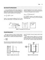
Fig. 12.4.24 Resistance of valves and fittings in terms of equivalent length of straight pipe. (Crane Co.)
Copyright (C) 1999 by The McGraw-Hill Companies, Inc. All rights reserved. Use of
this product is subject to the terms of its License Agreement. Click here to view.
12-98 AIR CONDITIONING, HEATING, AND VENTILATING
Table 12.4.40 Medium-Pressure Steam System (30 psig) Pipe Capacities (lb/h)
Pressure drop per 100 ft
Pipe
1
⁄
8
psi
1
⁄
4
psi
1
⁄
2
psi
3
⁄
4
psi 1 psi
size, in (2 oz) (4 oz) (8 oz) (12 oz) (16 oz)
Supply mains and risers 25–35 psig—max. error 8%
3
⁄
4
15 22 31 38 45

13146637789
1
1
⁄
4
69 100 141 172 199
1
1
⁄
2
107 154 219 267 309
2 217 313 444 543 627
2
1
⁄
2
358 516 730 924 1,033
3 651 940 1,330 1,628 1,880
3
1
⁄
2
979 1,414 2,000 2,447 2,825
4 1,386 2,000 2,830 3,464 4,000
5 2,560 3,642 5,225 6,402 7,390
6 4,210 6,030 8,590 10,240 12,140
8 8,750 12,640 17,860 21,865 25,250
10 16,250 23,450 33,200 40,625 46,900
12 25,640 36,930 52,320 64,050 74,000
Return mains and risers 0–4 psig—max. return pressure

3
⁄
4
115 170 245 308 365
1 230 340 490 615 730
1
1
⁄
4
485 710 1,025 1,285 1,530
1
1
⁄
2
790 1,155 1,670 2,100 2,500
2 1,575 2,355 3,400 4,300 5,050
2
1
⁄
2
2,650 3,900 5,600 7,100 8,400
3 4,850 7,100 10,250 12,850 15,300
3
1
⁄
2
7,200 10,550 15,250 19,150 22,750
4 10,200 15,000 21,600 27,000 32,250
5 19,000 27,750 40,250 55,500 60,000
4 31,000 45,500 65,500 83,000 98,000

Table 12.4.41 High-Pressure Steam System (150 psig) Pipe Capacities (lb/h)
Pressure drop per 100 ft
Pipe
1
⁄
8
psi
1
⁄
4
psi
1
⁄
2
psi
3
⁄
4
psi 1 psi 2 psi
size, in (2 oz) (4 oz) (8 oz) (12 oz) (16 oz) (32 oz) 5 psi
Supply mains and risers 130–180 psig—max, error 8%
3
⁄
4
29 41 58 82 116 184 300
1 58 82 117 165 233 369 550
1
1
⁄
4

130 185 262 370 523 827 1,230
1
1
⁄
2
203 287 407 575 813 1,230 1,730
2 412 583 825 1,167 1,650 2,000 3,410
2
1
⁄
2
683 959 1,359 1,920 2,430 3,300 5,200
3 1,237 1,750 2,476 3,500 4,210 6,000 9,400
3
1
⁄
2
1,855 2,626 3,715 5,250 6,020 8,500 13,100
4 2,625 3,718 5,260 7,430 8,400 12,300 19,200
5 4,858 6,875 9,725 13,750 15,000 21,200 33,100
6 7,960 11,275 15,950 22,550 25,200 36,500 56,500
8 16,590 23,475 33,200 46,950 50,000 70,200 120,000
10 30,820 43,430 61,700 77,250 90,000 130,000 210,000
12 48,600 68,750 97,250 123,000 155,000 200,000 320,000
Return mains and risers 1–20 psig—max, return pressure
3
⁄
4
156 232 360 465 560 890
1 313 462 690 910 1,120 1,780

1
1
⁄
4
650 960 1,500 1,950 2,330 3,700
1
1
⁄
2
1,070 1,580 2,460 3,160 3,800 6,100
2 2,160 3,300 4,950 6,400 7,700 12,300
2
1
⁄
2
3,600 5,350 8,200 10,700 12,800 20,400
3 6,500 9,600 15,000 19,500 23,300 37,200
3
1
⁄
2
9,600 14,400 22,300 28,700 34,500 55,000
4 13,700 20,500 31,600 40,500 49,200 78,500
5 25,600 38,100 58,500 76,000 91,500 146,000
6 42,000 62,500 96,000 125,000 150,000 238,000
Copyright (C) 1999 by The McGraw-Hill Companies, Inc. All rights reserved. Use of
this product is subject to the terms of its License Agreement. Click here to view.
12.5 ILLUMINATION
by Abraham Abramowitz
R

EFERENCES
: Amick, ‘‘Fluorescent Lighting Manual,’’ McGraw-Hill. ‘‘IES
Lighting Handbook’’ (1981). Design publications of General Electric Co., North
American Philips Co. (successor to Westinghouse Electric Co. Lamp Division),
and GTE-Sylvania.
BASIC UNITS
Candela, cd
(formerly candle) is the unit of luminous intensity of a light
source. One candela is defined as the luminous intensity in a given
direction, of a source that emits monochromatic radiation of frequency
540 ϫ 10
12
Hz (approximately 555 nm) and of which the radiant inten-
sity in that direction
1
⁄
683
W per steradian (W/sr).
Lumen, lm, is the unit of luminous flux
␾
. It is equal to the flux on a
unit surface all points of which are one unit distant from a uniform point
source of one candela. Such a point source emits 4
␲
lumens. (For an
additional definition of lumen, see the following material on vision.)
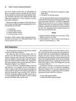
Illuminance E is the density of luminous flux on a surface. If the foot
is taken as the unit of length and the flux is uniformly distributed over
the surface, the density in
lumens per square foot is called footcandles, fc;

in SI units lumens per square metre, lux (lx), is used. (One footcandle
equals 10.76 lux.) In order to make the units comparable, dekalux
(10 lux) is frequently used.
The term illumination is frequently used for the word illuminance.
Modern practice reserves illumination for the process of lighting and
illuminance for the result.
Luminance is the luminance intensity of any surface in a given direc-
tion per unit of projected area of the surface as viewed from that direc-
tion. The unit of luminance is candela/in
2
; in SI units cd/m
2
is used.
(1 cd/in
2
ϭ 1,550 cd/m
2
.) In general, a luminous surface will have a
different luminance when viewed from different angles. An important
exception is a
perfectly diffuse reflecting (lambertian) surface which has a
constant luminance regardless of the viewing angle. If such a surface
has a luminance of 1 cd/in
2
, it emits 452 lm/ft
2
. Footlamberts, fL, in
lumens per square foot, is the unit of luminance applied to this case.
While this conversion applies only to the perfectly diffuse case, it is
frequently used in all cases. Thus, a perfectly diffuse surface with a

luminance of 1 cd/in
2
is said to have a luminance of 452 fL. In practice
the average lumens emitted per square foot of surface is taken to be the
footlamberts. This conversion practice is deprecated.
Subjective brightness is the subjective attribute of any light sensation
giving rise to the whole scale of qualities of becoming bright, light,
brilliant, dim, or dark. Unfortunately, the term ‘‘brightness’’ often is
used when referring to luminance.
N
OTE
. The above definitions are adapted from the ‘‘IES Lighting Hand-
book.’’
Absorption, reflection, and transmission
are the general processes by
which incident light flux interacts with a medium.
Absorption is the
process whereby incident flux is dissipated.
Reflection is the process by
which the incident flux leaves a surface or medium from the incident
side.
N
OTE
. Reflection may occur as from a mirror (specular reflection), it may be
reflected at angles different from that of the incident fluxto incident plane (diffuse
reflection), or it may be a combination of the two types of reflection.
Transmission
is the process by which incident flux leaves a surface or
medium on a side other than the incident side. If the light ray is reduced
only in intensity, the transmission iscalledregular. If the rayemergesin

all directions, transmission is called diffuse. Both modes may exist in
combination.
The incident flux
␾
i
equals the flux absorbed
␾
a
, reflected
␾
r
, and
transmitted
␾
t
. That is,
␾
i
ϭ
␾
a
ϩ
␾
r
ϩ
␾
t
Dividing this equation by
␾
i

, we obtain
1 ϭ
␾
a
/
␾
i
ϩ
␾
r
/
␾
i
ϩ
␾
t
/
␾
i
or 1 ϭ
␣
ϩ
␳
ϩ
␶
␣
is the absorptance,
␳
is the reflectance, and
␶

is the transmittance. In
each case, the incident flux may be restricted to a single wavelength, a
particular direction, and a given solid angle. These must be specified.
The
wavelength of electromagnetic radiation is measured in metres.
For the frequencies involved in illumination, the wavelength is given in
nanometres, nm, equal to 10
Ϫ9
m, and micrometres,
␮
m, equal to
10
Ϫ6
m.
VISION
Most engineering designs, (bridges, structures, roads etc.) are based on
strength and are not concerned with the way the human organism reacts.
The
response of the eye is central to illuminating engineering. The lens of
the
eye focuses an image on the retina. Here a photochemical process
takes place which sends nerve impulses to the brain via the optic nerve.
The amount of light entering the eye is controlled by the
pupil. The
normal eye automatically accommodates itself to focus on an object,
while the pupil adjusts itself to allow for a high or low level of object
luminance. The sensors in the eye are known as
rods and cones. The
cones are clustered in a small central part of the retina called the
fovea.

They transmit a sharp image to the brain and give color response. Out-
side the fovea the rods predominate. They give neither a sharp image
nor a color response. When the luminance of the visual field is 0.01 fL
or lower, as at night, seeing is due to the rods only and is called
scotopic
vision.
At higher levels, with the cones primarily involved, seeing is
called
photopic vision. There is an intermediate region called mesopic
vision.
The response of the eye to colors of different wavelengths is given in
Fig. 12.5.1. Note the shift in maximum response at lower luminance
levels called the ‘‘Purkinje shift.’’ Note that these curves are relative
ones, and that the two peaks do not correspond to the same levels of
illumination. The
luminous efficacy (lumen output per radiated watt) is
683 lm/W at the wavelength of maximum photopic response 555 nm.
For white light, radiation which has the characteristicofan equal energy
spectrum with all the energy in the visualregion,it is approximately 220
lm/W.
Spectral Lumen If the response curve of the eye for photopic vi-
sion, versus
␭
in nanometers, is expressed as k(
␭
), and the spectral
power function of the source in watts per nanometer is taken to be
Q
e
(

␭
), then the luminous flux is given by the equation
␾
lumens
ϭ 683
͵
780
380
k(
␭
) Q
e
(
␭
) d(
␭
) (12.5.1)
LIGHT METERS
Early light meters compared the luminance of a diffuse highly reflecting
surface with that obtained from a calibrated standard. The most com-
mon light meter in use today is similar to a photographic exposure
meter. A photovoltaic cell is directly connected to a sensitive microam-
meter calibrated in footcandles (or dekalux). The best meters (called
color-corrected) have a response similar to that of the eye in photopic
vision. Special shapes are used on the cover to avoid total reflection of
12-99
Copyright (C) 1999 by The McGraw-Hill Companies, Inc. All rights reserved. Use of
this product is subject to the terms of its License Agreement. Click here to view.
12-100 ILLUMINATION
Fig. 12.5.1 Relative spectral luminous efficiency curves for photopic and sco-

topic vision, showing the Purkinje shift on the wavelength of maximum effi-
ciency. Note the wavelength of the visual region of the electromagnetic spectrum.
(IESNA Lighting Handbook, 5th ed. This material has been modified from its
original version and is not reflective of its original form as recognized by the
IESNA.)
light from the glass surface of the cell. Such meters are said to be cosine
law corrected. The microammeter is frequently replaced with an elec-
tronic amplifier using an analog or digital readout.
LIGHT SOURCES
The original and still major source of light is the sun. Next came fire,
derived from candles, oil, and gas lamps. With the discovery of electric-
ity came arc lamps, gas-discharge lamps, and hot-filament lamps.
‘‘Flame’’ or hot sources give a continuous spectrum. Gas-discharge
devices such as neon lamps and mercury-arc lamps give discrete, or
line, spectra. The lines may be modified in various ways: by pressure
broadening, use of phosphor coatings (to convert ultraviolet radiation
into visible light), and using a mixture of gases. The continuous spectra
of phosphors have colors which depend upon the mixture used. Light-
emitting diodes, LED, consisting of a layer of two different semicon-
ductors, are in use for display purposes.
Color Temperature and Luminance
In general, three quantities are required to specify the color of a light
and its luminous level. However, an approximate designation is used by
specifying the temperature of a hot (black-body) emitter whose color
almost matches that of the light. The
color temperature of daylight is
about 6000 K and that of tungsten lamps about 2300 to 3300 K.
Table 12.5.1 Approximate Luminances of Various Light
Sources (IES)
Approximate average

luminance
Light source cd/in
2
kcd/m
2
Clear sky 5.16 8
Candle flame (sperm) 6.45 10
60-W inside frosted bulb 77.4 120
60-W ‘‘white bulb’’ 19.35 30
Fluorescent lamp, cool white, T-12
bulb, medium loading
5.3 8.2
High-intensity mercury-arc type H33,
2.5 atm
968 1,500
Clear glass neon tube 15 mm, 60 mA 1.03 1.6
Different light sources have markedly different luminances as shown
in Table 12.5.1. ‘‘Large’’ sources have low luminances, while ‘‘small’’
sources have high luminances.
Lamps
Electric lamps are the principal source of artificial light in common use.
They convert electrical energy into light or radiant energy.
An
incandescent-filament lamp contains a filament which is heated by
the current passing through it. The filament is enclosed in a glass bulb
which has a base suitable to connect the lamp to an electrical socket. To
prevent oxidation of the filament at elevated temperature, the bulb is
evacuated of air or filled with an inert gas. The bulb also serves to
control the light from the incandescent filament, which is essentially a
point source. High luminance of the source is typically reduced by acid

etching to frost the inside surface of the bulb. Silica coating will also
provide additional diffusion and can alter the color of the light emitted.
Portions of the bulb’s interior can be covered with reflecting material to
give a predetermined direction to the emitted light. Chemical tinting of
clear glass bulbs provides a variety of colors. Whenever the color that is
normally produced by an incandescent filament is changed, the filtering
process removes from the radiated light the energy of all wavelengths
except those necessary to produce the desired color. This subtractive
method of color alteration is less efficacious than the generation of light
of varying colors by gaseous discharge.
Sizes and shapes of lamp bulbs are designated by a letter code fol-
lowed by a numeral; the letter indicates the shape (Fig. 12.5.2), and the
number indicates the diameter of the bulb in eighths of an inch. Thus a
T-12 lamp has a tubular shape and is 1
4
⁄
8
or 1
1
⁄
2
in in diameter.
Fig. 12.5.2 Typical filament lamp shapes: S, straight; F, flame; G, globe;
A, general service; T, tubular; PS, pear shape; PAR, parabolic; R, reflector.
Incandescent lamps
are available with several types of bases (Fig.
12.5.3). Most general-service lamps have medium screw bases; larger
or smaller screw bases are used depending on lamp wattage. Bipost and
prefocus bases accurately position the filament, as in optical projection
systems. Bipost lamps also serve where ruggedness and greater heat

dissipation are required.
Fig. 12.5.3 Typical incandescent lamp bases.
Incandescent-lamp filaments are generally constructed of tungsten.
Tungsten has a high melting point and a low vapor pressure, which
permits high operating temperatures without evaporation: the higher the
operating temperature, the higher the efficacy (lumens per watt) and the
shorter the life. Filament evaporation throughout the life of the lamp
causes blackening of the bulb and thinning of the filament with conse-
quent lower light output. Argon-nitrogen gas filling reduces the rate of
evaporation. Figure 12.5.4 shows steps in lamp manufacture.
Tungsten filaments are also placed in compact quartz tubes filled
with a halogen atmosphere where the tungsten halide lighting source
Copyright (C) 1999 by The McGraw-Hill Companies, Inc. All rights reserved. Use of
this product is subject to the terms of its License Agreement. Click here to view.
12-102 ILLUMINATION
high wattage losses at the electrodes. They are limited to low current
densities because the electrodes operate at temperatures below that nec-
essary for thermionic emission. Cold-cathode lamps, whose operation is
not affected by dimming or flashing, have long life and are generally
used for custom-built shapes and patterns that require bending, such as
for electric signs.
Fig. 12.5.7 Starter switches for preheat cathode circuits. (IESNA)
Rapid-start
circuit ballasts have separate windings for the electrodes
which are immediately and continuously heated when the circuit is
energized. This rapid heating causes sufficient ionization in the lamp for
a discharge to start from the voltage of the main ballast windings. Two-
lamp rapid-start ballasts are of the series sequence type, in which the
lamps start in sequence and, when fully lighted, operate in series.
A new type

screw-in fluorescent lamp with built-in ballast can be used
in a standard medium-screw socket. These lamps consume less power
than incandescent lamps for the same luminance; accordingly, albeit
their first cost is significantly higher, they are expected to prove to be
more economical by virtue of their reduced power consumption and
much longer life. The verdict of the consuming public is yet to come as
significant numbers of them make their way into household and com-
mercial applications.
Fluorescent lamps used in low-ambient-temperature applications, as
in outdoor signs, are of the
high-output (HO) type, and require special
high-output ballasts to permit the lamps to maintain their luminance at
lower operating temperatures.
Typical fluorescent lamp circuits are shown in Fig. 12.5.8.
High-intensity-discharge lamps consist of tubes in which electric arcs
in a variety of materials are produced. Outer glass jackets provide ther-
mal insulation in order to maintain the arc tube temperature. The tem-
perature and amount of material is controlled so that the discharge oper-
ates in a vapor pressure of several atmospheres. This results in
enhancing the radiation in the visible region.
Mercury-vapor lamps consist of mercury-argon-filled quartz tubes
surrounded by a nitrogen-filled glass jacket. Clear lamps radiate the
visible mercury lines (bluish green). Ultraviolet radiation is absorbed to
some extent by the outer jackets. The color of the light and the lumen
output is improved by coating the inside of the outer jackets with a
phosphor. When excited by the ultraviolet radiation of the arc, the phos-
phors add light in the red part of the spectrum to the output. The result-
ing lamps are called white, color improved, or deluxe white. The lamps
start by a discharge in argon between an electrode and a starting elec-
trode (see Fig. 12.5.9). As the mercury vaporizes, the pressure builds up

and the discharge transfers to a mercury discharge. This takes several
minutes. After shutdown, the lamps cannot be restarted until the inner
tube pressure drops so that an argon discharge can start.
Metal halide (multivapor) lamps use small quantities of sodium, thal-
lium, scandium, dysprosium, and indium iodides in addition to the usual
mercury-argon mix. Color is improved and output substantially in-
creased over high-intensity-discharge lamps using mercury alone.
While the construction is similar to mercury lamps, a bimetal switch is
built into the lamp to short out the starting resistor after the lamps start.
A vacuum jacket is used around the quartz discharge tube (see Fig.
12.5.9).
High-pressure sodium-vapor lamps use metallic sodium sealed in trans-
lucent aluminum oxide tubes. This material is used to withstand the
corrosive effect of hot sodium vapor. For starting purposes a xenon fill
gas and a sodium-mercury amalgam is used. Arc temperatures are
maintained by an outer vacuum jacket. The lamp is started by generat-
ing a high-voltage pulse for about a microsecond (see Fig. 12.5.9).
High-pressure discharge lamps, like fluorescent lamps, require bal-
lasts. These provide the necessary voltage, reactances, and power-
factor-correcting capacitors. Typical circuits are shown in Fig. 12.5.8.
Table 12.5.2 Comparable Luminous
Efficacies (lumens/watt)* (IES)
Lamp Lumens/watt
Tungsten incandescent 8–33
High-intensity mercury† 24–63‡
Fluorescent† 19–100‡
Metal halide (multivapor)† 69–125
High-pressure sodium† 73–140
* Constantly being improved.
† Ballast losses not included.

‡ Depends upon lamp size, type, and color.
Comparative lamp efficacies (lumens/watt) are given in Table
12.5.2. Lamp data for commonly used incandescent, fluorescent, and
high-intensity-discharge lamps are listed in Tables 12.5.3, 12.5.4, and
12.5.5.
Luminaires
Luminaires are generally categorized as industrial, commercial, or resi-
dential.
Use within these categories usually determines the quality
and ruggedness of materials of construction. Generally speaking,
style, ornament, and in most cases low cost are prime considerations for
residential fixtures. Industrial fixtures require low maintenance, low
operating cost, efficiency, and durability. Commercial fixtures combine
the elements of all of these and place heavy emphasis on visual
comfort.
Luminaires are classified by the International Commission on Illumi-
nation (ICI) in accordance with the percentages of total luminaire out-
put emitted above and below the horizontal (Fig. 12.5.10). Industrial
fixtures usually are direct or semidirect.
Table 12.5.3 Incandescent-Lamp Data
Watts Bulb size Initial lumens Rated life, h
25 A-19 230 2,500
40 A-19 474 1,500
60 A-19 1,060 1,000
75 A-19 1,190 750
100 A-19 1,740 750
150 A-21 2,873 750
200 A-23 4,000 750
300 PS-30 6,130 750
500 PS-35 10,675 1,000

750 PS-52 16,935 1,000
1,000 PS-52 23,510 1,000
For general-service lamps 115-, 120-, and 125-V service, inside frosted.
N
OTE
: Lamps are constantly being improved. The latest manufacturer’s data should be used
for accuracy.
S
OURCE
: ‘‘IESNA Handbook,’’ 8th ed., 1993, reprinted with permission. (This material has
been modified from its originalversion and is not reflective ofits original formas recognized by
the IESNA.)
Copyright (C) 1999 by The McGraw-Hill Companies, Inc. All rights reserved. Use of
this product is subject to the terms of its License Agreement. Click here to view.
12-104 ILLUMINATION
Table 12.5.4 Fluorescent Lamp Data*
Rated
Single-lamp Two-lamp Cool white
average life,
Nominal length
Approx lamp
circuit watts circuit watts lumens at
h
Lamp Current 3h
designation mm in (ma) Volts Watts Ballast Total Ballast Total 100 h burning/start
Preheat starting†
F15T12 450 18 325 47 15 4.5 19.5 9 39 830 9,000
F20T12 600 24 380 57 20.5 5 25.5 10 51 1,283 9,000
F30T8 900 36 355 99 30.5 10.5 41 17 78 2,330 7,500
F40T12 1,200 48 430 101 40 12 52 16 96 2,150 15,000

F90T12 1,500 60 1,500 65 90 20 110 24 204 6,025 9,000
Rapid start† (lightly loaded lamps)
F30T12 900 36 430 81 33.5 10.5 44 2,210 18,000
F40T12 1,200 48 430 101 41 13 54 13 95 3,150 21,000
Rapid start† (medium loaded lamps)
F48T12 1,200 48 800 78 63 85 146 4,300 12,000
F72T12 1,800 72 800 117 87 106 200 6,650 12,000
F96T12 2,400 96 800 153 113 140 252 9,150 12,000
Rapid start† (highly loaded lamps and power grove§)
F48T12/48PG17 1,200 48 1,500 84 116 146 252 6,900/7,450 9,000
F72T12/72PG17 1,800 72 1,500 125 168 213 326 10,640/11,500 9,000
F96T12/96PG17 2,400 96 1,500 163 215 260 450 15,250/16,000 9,000
Instant start† (slimline)
F48T12 lead/lag 1,200 48 425 100 39 26 104 3,000 7,500–12,000
F48T12 series 1,200 48 425 100 39 17 95 3,000 7,500–12,000
F72T12 lead/lag 1,800 72 425 149 57 47 161 4,585 7,500–12,000
F72T12 series 1,800 72 425 149 57 25 139 4,585 7,500–12,000
F96T12 lead/lag 2,400 96 425 197 75 40 190 6,300 12,000
F96T12 series 2,400 96 425 197 75 22 172 6,300 12,000
Circline lamps¶
C8T9 200 OD 8
1
⁄
4
OD 370 61 22.5 7.5 30 1,065 12,000
C12T9 300 OD 12 OD 425 81 33 9 42 1,870 12,000
C16T9 400 OD 16 OD 415 108 41.5 16.5 58 2,580 12,000
S
OURCE
: Adapted from‘‘IESNA Handbook,’’ 8th ed., 1993, reprinted with permission. (This material has been modified from its original version and is not reflective of its original form as

recognized by the IESNA.)
* Lamps are continuously being improved. For design purposes consult the latest manufacturers’ data. Data shown is for standard lamps. Energy-saving ballastsand fluorescent lamps are available.
† The first number is the ‘‘nominal’’ lamp wattage, while the second number is the tube diameter in eighths of an inch.
§ General Electric Co. trademark.
¶ The first number is the nominal outside diameter of the lamp, while the second number is the tube diameter in eighths of an inch.
Table 12.5.5 High-Intensity-Discharge Lamp Data*
Nominal lamp
Watt Voltage Amperes
Approx
ballast
loss, watts
Approx initial
lumens† (100 h) Life, h
Mercury lamps
100 130 0.85 10–35 2,500–4,400 24,000ϩ
175 130 1.5 15–35 6,000–8,600 24,000ϩ
250 130 2.1 25–35 8,000–13,000 24,000ϩ
400 135 3.2 20–55 15,000–23,000 24,000ϩ
700 265 2.8 35–65 36,000–43,000 24,000ϩ
1,000 265 4.0 40–90 43,000–63,000 24,000ϩ
Metal-halide lamps
175 130 1.4 35 12,000–14,000 7,500
400 135 3.2 60 31,000–40,000 15,000–20,000
1,000 250 4.3 50–100 105,000–125,000 10,000–12,000
High-pressure sodium-vapor lamps
250 100 3.0 55–60 25,000–30,000 24,000
400 100 4.7 65–75 47,500–50,000 24,000
S
OURCE
: Abstracted from ‘‘IES Lighting Handbook’’ and General Electric Co. data.

* Lamps are continuously being improved. For design purposes, consult the latest manufacturers’ data.
† Depending upon ballast used, lamps may have outputs which change with burning position.
Copyright (C) 1999 by The McGraw-Hill Companies, Inc. All rights reserved. Use of
this product is subject to the terms of its License Agreement. Click here to view.
12-106 ILLUMINATION
matte surface without shining details, and light should come from the
side or behind the worker.
In addition to veiling reflectance, there is a reduction in contrast due
to light directly entering the eye from the source. This is called the
disability glare effect. It produces a light veil over the image of the task
on the retina. It is not a serious problem in interior lighting, but it is
important in roadway lighting and similar situations.
Visual-Comfort Criteria High luminances directly or reflected in
the field of view can cause discomfort without necessarily interfering
with seeing even though visual performance may be impaired. This
discomfort glare can be caused by direct glare from sources which have
too high a luminance, are inadequately shielded, or have too great
an area. Lighting systems are rated by a
visual-comfort probability,
VCP,
expressed as a percentage of people who, if seated in the most
undesirable location, will be expected to find it acceptable. (For a com-
plete description of VCP, see the IESNA Handbook.) If the following
conditions are met, direct glare will not be a problem in lighting instal-
lations:
1. The VCP is 70 or more.
2. The ratio of maximum-to-average luminaire luminance does not
exceed 5 :1 (preferably 3:1) at 45, 55, 65, 75, and 85° from the nadir
crosswise and lengthwise.
3. Maximum luminaire luminances crosswise and lengthwise do not

exceed the following values:
Angle above
Maximum luminance
nadir, deg cd/m
2
fL
45 7,710 2,250
55 5,500 1,605
65 3,860 1,125
75 2,570 750
85 1,695 495
Design of Interior Lighting Systems
Lighting is as much an art as a science. While many studies have been
made on what constitutes adequate lighting along with proper quality,
the effect to be achieved depends upon the designer. In this section
emphasis will be primarily on achieving adequate illumination.
The design approach is to consider the spacetobe lighted and thetask
to be performed. An illuminance is then selected. Asuitableluminaireis
picked, and calculations are made in order to determine the number and
layout of the fixtures. The overall quality is then checked. If unsatisfac-
tory, a new layout is made. Aneconomicstudy is made tocheckcosts. If
these are too high, new layouts are studied until all design restraints
are met.
Selection of illuminance Levels
From 1958, the Illuminating Engineering Society (IES) published
single-value illuminance levels. Their latest publication, the 1993
‘‘IESNA Lighting Handbook,’’ gives a range of values which permits
lighting designers to tailor lighting systems to specific needs. This flex-
ibility permits levels to be adjusted for (1) the visual task; (2) the age of
the observers; (3) the need for speed and/or accuracy for visual per-

formance; (4) the reflectance of the task. An illumination-level guide
for selected tasks is given in Table 12.5.6. The data are based on an
assumption of average conditions for people, tasks, and visual perfor-
mance requirements. For other conditions see the 1993 ‘‘IESNA Light-
ing Handbook.’’
Room, Furniture, and Equipment Finishes
The color and finish of rooms, furniture, and equipment are important in
the overall lighting design. Best results are obtained when the lighting
designer coordinates his or her work with the architect, interior decora-
tor, or plant designer.
Table 12.5.6 Illuminance Guide for Selected Tasks
Footcandles
(lm/ft) Lux (lm/m
2
)
Commercial drafting
Conventional 150* 1,600*
Libraries
Reading good print, typed originals 30 320
Reading small print, handwriting, pho-
tocopies
75 800
Active stacks (vertical, illumination) 30 320
Offices
Conference rooms—conferring 30 320
Conference rooms—typical visual tasks 75–100 800–1,080
Corridors, stairs, elevators 20 220
General tasks, varying difficulty 100 1,080
Lobbies, reception areas 30 320
Private 75 880

Rest rooms 30 320
Video display areas 75 800
School
Classrooms, laboratories 75 800
Shops 100 1,080
Sight-saving rooms, hearing-impaired
classes
150 1,600
Store
Mass merchandizing, high activity 100 1,080
Self-service 200 2,200
Circulation, low activity 30 320
Feature displays, low, medium, 1,600,* 3,200*,
high activity
150,* 300,* 500*
5,400*
Industrial
Garages
Repair 75 800
Active traffic areas 15 160
Loading platform 20 220
Machine shops and assembly areas
Rough bench-machine work, simple
assembly
50 540
Medium bench-machine work, mod-
erately difficult assembly
100* 1,080*
Difficult machine work, assembly 150* 1,600*
Fine bench-machine work, assembly 300* 3,200*

Receiving and shipping 30 320
Warehouse storage rooms
Active large items 15 160
Active small items, labels 30 320
Inactive 5 54
Outdoor areas
Storage yards
Active 20 220
Inactive 1 11
Parking areas
Open, high activity 2 22
Open, medium activity 1 11
Covered parking, pedestrian areas 5 54
Covered night entrance 5 54
Covered day entrance 50 54
S
OURCE
: Adapted from General Electric Co. design data.
* Requires supplementary lighting. Care should be taken thatthe supplementarylighting does
not introduce direct and reflected glare.
Copyright (C) 1999 by The McGraw-Hill Companies, Inc. All rights reserved. Use of
this product is subject to the terms of its License Agreement. Click here to view.
LIGHTING DESIGN 12-107
A color scheme should be selected to give light reflectance values as
follows:
Percent
Area or unit reflectance
Ceilings 70–90
Floors 20–40*
Walls, draperies 40–60†

Bench top, desks, machine, and equipment 25–45
* In storage areas, keep reflectance of aisle floors as high as possible
in order to reflect light onto the lower shelves. This should also be done
where the underside of objects has to be seen.
† These values should be 30 to 40 where video display terminals
(VDTs) are used to avoid veiling reflections in the VDT faces.
The color and finish of a space and equipment therein sets the psy-
chological feel of the space. For example, the trend is away from drab
finishes on machinery and dark gray filing cabinets. Colors such as
yellow, orange, red, and light gray seem to advance toward the eye.
They tend to make large spaces feel smaller. Receding colors such as
violet, blue, blue green, and dark grays make small spaces feel larger.
Some colors are used for safety purposes. Various areas are painted to
designate safe or hazardous locations in a fashion similar to piping
identification discussed in Sec. 8. These colors have been carefully
standardized in ANSI Z53.1-1979.
Designating Color
In order to be able to obtain designed values of a lighting system, it is
necessary to be able to specify the exact color wanted. Many methods
have been devised for so doing. One method uses carefully controlled
sets of colored chips, each one of which has a particular designation.
The desired color is matched against these chips. The
Munsell system
uses scales of hue (the actual basic color such as red), value (a 10-step
scale ranging from black through grays to white), and chroma (the
amount of gray mixed in with the color). This system is used by many
manufacturers to designate their colors. The
Ostwald system describes
color in terms of color content, white content, and black content. The
Inter-Society Color Council–National Bureau of Standards (ISCC-NBS)

method designates one-inch square samples with names. For color des-
ignation by the
ICI method, a spectroradiometric curve of the source is
determined together with a spectrophotometric curve of the reflecting or
transmitting surface. By mathematical manipulation using spectral tri-
stimulus values, chromaticity coordinates are obtained. See the IESNA
Handbook for details. Chromaticity coordinates are extensivelyusedfor
fluorescent lamp colors. These coordinates can be measured directly by
photoelectric colorimeters. They are designed with filter photocell re-
sponses to be close to each of the ICI tristimulus values. Built-in logic
circuitry results in direct reading of the chromaticity. Incandescent and
vapor-type lamp colors are specified by color temperature.
LIGHTING DESIGN
Interior lighting is designed by the lumen method. This takes into ac-
count the interreflections of light inside a room. The average illumin-
ance on the work plane equals the incident luminous flux
␾
divided by
the area, or E ϭ
␾
/A. Lumens reaching the work plane is equal to lamp
lumens multiplied by the
coefficient of utilization CU. This factor is a
function of room size, shape, and finish, mounting height of fixture, and
type of luminaire used. The lumens
␾
L
initially available from the
lamps may be reduced by ambient temperature, lower voltage, and the
ballast used. As time goes by the room surfaces and luminaires become

dirty, which further reduces the illuminance. In addition, lamp output
falls, and some of them burn out. The total effect of all these factors is
expressed by the light-loss factor LLF. The maintained illuminance E
m
is the initial illumination times the LLF, or
E
m
ϭ (
␾
L
ϫ CU ϫ LLF)/A (12.5.5)
The required maintained illuminance is selected from Table 12.5.6 or
from the more extensive data in the IESNA Handbook. A fixture and
lamp is selected, and Eq. (12.5.5) is solved for the necessary lamp flux
␾
L
. The number of luminaires N is found by dividing the total lamp
lumens
␾
L
by the lumens per fixture
␾
F
. A trial layout is then made. A
simple layout keeps spacing between units equal to twice the distance
between fixtures and wall. Spacing is checked against the maximum
allowable luminaire spacing from manufacturers’ data to ensure uni-
form illumination. However, this criterion results in inadequate lighting
near the walls. In order to light desks and benches along the walls, a
spacing of 2

1
⁄
2
ft from the luminaire center to the wall is used. The ends
of fluorescent luminaire rows should be 6 to 12 in from the walls with a
maximum distance of 2 ft.
Wall and ceiling cavity luminances can be obtained by using lumi-
nance coefficients (LC) for the fixtures (see the IESNA Handbook). For
interior areas, maximum luminance ratios should be 3: 1 or 1:3 be-
tween tasks and immediate surround, and 10 :1 or 1 :10 between tasks
and remote surfaces. To ensure eye comfort, the visual-comfort proba-
bility (VCP) is investigated.
The
coefficient of utilization is found by using the zonal-cavity method.
In this method effects of the room proportion, luminaire suspension
lengths, and work-plane height on the CU are found by dividing the
room into three cavities as shown in Fig. 12.5.11. For each cavity a
cavity ratio is calculated:
Cavity ratio ϭ
5h (room length ϩ room width)
(room length) ϫ (room width)
(12.5.6)
where h ϭ h
RC
for the room cavity ratio RCR; ϭ h
CC
for the ceiling
cavity ratio CCR; and ϭ h
FC
for the floor cavity ratio FCR.

Fig. 12.5.11 The three cavities used in the zonal cavity method.
Table 12.5.7 is used to obtain a single effective ceiling cavity reflec-
tance
␳
CC
and a single effective floor cavity reflectance
␳
FC
. For
surface-mounted and recessed luminaires, CCR ϭ 0 and the ceiling
reflectance is used as
␳
CC
. Figure 12.5.12 gives CU for selected fix-
tures. In using Fig. 12.5.12, interpolation may be necessary. Additional
fixture data are given in the IES Handbook. Fixture manufacturers fur-
nish such data for their units. Those data should be used for the best
accuracy. If the effective floor cavity reflectance
␳
FC
differs from 20
percent, an adjustment is made by using Table 12.5.8.
For simplicity in calculating the light-loss factor, the effects of am-
bient temperature, luminaire voltage variation, ballasts, and burnouts
will be neglected. Room-surface dirt depreciation factors are shown in
Fig. 12.5.13; luminaire dirt depreciation factors are in Fig. 12.5.14. The
importance of frequent cleaning is evident. Categories are given for
each fixture in Fig. 12.5.12. Lamp lumen depreciation (LLD) depends
upon when lamps are replaced before complete burnout. If replacement
Copyright (C) 1999 by The McGraw-Hill Companies, Inc. All rights reserved. Use of

this product is subject to the terms of its License Agreement. Click here to view.
Table 12.5.7 Percent Effective Ceiling or Floor Cavity Reflectance for Various Reflectance Combinations (Continued)
% base*
reflectance: 40 30 20 10 0
% wall
Cavity reflectance:
ratio 90 80 70 60 50 40 30 20 10 0 90 80 70 60 50 40 30 20 10 0 90 80 70 60 50 40 30 20 10 0 90 80 70 60 50 40 30 20 10 0 90 80 70 60 50 40 30 20 10 0
0.2 40 40 39 39 39 38 38 37 36 36 31 31 30 30 29 29 29 28 28 27 21 20 20 20 20 20 19 19 19 17 11 11 11 10 10 10 10 09 09 09 02 02 02 01 01 01 01 00 00 0
0.4 41 40 39 39 38 37 36 35 34 34 31 31 30 30 29 28 28 27 26 25 22 21 20 20 20 19 19 18 18 16 12 11 11 11 11 10 10 09 09 08 04 03 03 02 02 02 01 01 00 0
0.6 41 40 39 38 37 36 34 33 32 31 32 31 30 29 28 27 26 26 25 23 23 21 21 20 19 19 18 18 17 15 13 13 12 11 11 10 10 09 08 08 05 05 04 03 03 02 02 01 01 0
0.8 41 40 38 37 36 35 33 32 31 29 32 31 30 29 28 26 25 25 23 22 24 22 21 20 19 19 18 17 16 14 15 14 13 12 11 10 10 09 08 07 07 06 05 04 04 03 02 02 01 0
1.0 42 40 38 37 35 33 32 31 29 27 33 32 30 29 27 25 24 23 22 20 25 23 22 20 19 18 17 16 15 13 16 14 13 12 12 11 10 09 08 07 08 07 06 05 04 03 02 02 01 0
1.2 42 40 38 36 34 32 30 29 27 25 33 32 30 28 27 25 23 22 21 19 25 23 22 20 19 17 17 16 14 12 17 15 14 13 12 11 10 09 07 06 10 08 07 06 05 04 03 02 01 0
1.4 42 39 37 35 33 31 29 27 25 23 34 32 30 28 26 24 22 21 19 18 26 24 22 20 18 17 16 15 13 12 18 16 14 13 12 11 10 09 07 06 11 09 08 07 06 04 03 02 01 0
1.6 42 39 37 35 32 30 27 25 23 22 34 33 29 27 25 23 22 20 18 17 26 24 22 20 18 17 16 15 13 11 19 17 15 14 12 11 09 08 07 06 12 10 09 07 06 05 03 02 01 0
1.8 42 39 36 34 31 29 26 24 22 21 35 33 29 27 25 23 21 19 17 16 27 25 23 20 18 17 15 14 12 10 19 17 15 14 13 11 09 08 06 05 13 11 09 08 07 05 04 03 01 0
2.0 42 39 36 34 31 28 25 23 21 19 35 33 29 26 24 22 20 18 16 14 28 25 23 20 18 16 15 13 11 09 20 18 16 14 13 11 09 98 06 05 14 12 10 09 07 05 04 03 01 0
2.2 42 39 36 33 30 27 24 22 19 18 36 32 29 26 24 22 19 17 15 13 28 25 23 20 18 16 14 12 10 09 21 19 16 14 13 11 09 07 06 05 15 13 11 09 07 06 04 03 02 0
2.4 43 39 35 33 29 27 24 21 18 17 36 32 29 26 24 22 19 16 14 12 29 26 23 20 18 16 14 12 10 08 22 19 17 15 13 11 09 07 06 05 16 13 11 09 08 06 04 03 01 0
2.6 43 39 35 32 29 26 23 20 17 15 36 32 29 25 23 21 18 16 14 12 29 26 23 20 18 16 14 11 09 08 23 20 17 15 13 11 09 07 06 04 17 14 12 10 08 06 05 03 02 0
2.8 43 39 35 32 28 25 22 19 16 14 37 33 29 25 23 21 17 15 13 11 30 27 23 20 18 15 13 11 09 07 23 20 18 16 13 11 09 07 05 03 17 15 13 10 08 07 05 03 02 0
3.0 43 39 35 31 27 24 21 18 16 13 37 33 29 25 22 20 17 15 12 10 30 27 23 20 17 15 13 11 09 07 24 21 18 16 13 11 09 07 05 03 18 16 13 11 09 07 05 03 02 0
3.2 43 39 35 31 27 23 20 17 15 13 37 33 29 25 22 19 16 14 12 10 31 27 23 20 17 15 12 11 09 06 25 21 18 16 13 11 09 07 05 03 19 16 14 11 09 07 05 03 02 0
3.4 43 39 34 30 26 23 20 17 14 12 37 33 29 25 22 19 16 14 11 09 31 27 23 20 17 15 12 10 08 06 26 22 18 16 13 11 09 07 05 03 20 17 14 12 09 07 05 03 02 0
3.6 44 39 34 30 26 22 19 16 14 11 38 33 29 24 21 18 15 13 10 09 32 27 23 20 17 15 12 10 08 05 26 22 19 16 13 11 09 06 04 03 20 17 15 12 10 08 05 04 02 0
3.8 44 38 33 29 25 22 18 16 13 10 38 33 28 24 21 18 15 13 10 08 32 28 23 20 17 15 12 10 07 05 27 23 19 17 14 11 09 06 04 02 21 18 15 12 10 08 05 04 02 0
4.0 44 38 33 29 25 21 18 15 12 10 38 33 28 24 21 18 14 12 09 07 33 28 23 20 17 14 11 09 07 05 27 23 20 17 14 11 09 06 04 02 22 18 15 13 10 08 05 04 02 0
4.2 44 38 33 29 24 21 17 15 12 10 38 33 28 24 20 17 14 12 09 07 33 28 23 20 17 14 11 09 07 04 28 24 20 17 14 11 09 06 04 02 22 19 16 13 10 08 06 04 02 0
4.4 44 38 33 28 24 21 17 14 11 09 39 33 28 24 20 17 14 11 09 06 34 28 24 20 17 14 11 09 07 04 28 24 20 17 14 11 08 06 04 02 23 19 16 13 10 8 06 04 02 0
4.6 44 38 32 28 23 19 16 14 11 08 39 33 28 24 20 17 13 10 08 06 34 29 24 20 17 14 11 09 07 04 29 25 20 17 14 11 08 06 04 02 23 20 17 13 11 08 06 04 02 0

4.8 44 38 32 27 22 19 16 13 10 08 39 33 28 24 20 17 13 10 08 05 35 29 24 20 17 13 10 08 06 04 29 25 20 17 14 11 08 06 04 02 24 20 17 14 11 08 06 04 02 0
5.0 45 38 31 27 22 19 15 13 10 07 39 33 28 24 19 16 13 10 08 05 35 29 24 20 16 13 10 08 06 04 30 25 20 17 14 11 08 06 04 02 25 21 17 14 11 08 06 04 02 0
6.0 44 37 30 25 20 17 13 11 08 05 39 33 27 23 18 15 11 09 06 04 36 30 24 20 16 13 10 08 05 02 31 26 21 17 14 11 08 06 03 01 27 23 18 15 12 09 06 04 02 0
7.0 44 36 29 24 19 16 12 10 07 04 40 33 26 22 17 14 10 08 05 03 36 30 24 20 15 12 09 07 04 02 32 27 21 17 13 11 08 06 03 01 28 24 19 15 12 09 06 04 02 0
8.0 44 35 28 23 18 15 11 09 06 03 40 33 26 21 16 13 09 07 04 02 37 30 23 19 15 12 08 06 03 01 33 27 21 17 13 10 07 05 03 01 30 25 20 15 12 09 06 04 02 0
9.0 44 35 26 21 16 12 10 08 05 02 40 33 25 20 15 12 09 07 04 02 37 29 23 19 14 11 08 06 03 01 34 28 21 17 13 10 07 05 02 01 31 25 20 15 12 09 06 04 02 0
10.0 43 34 25 20 15 12 08 07 05 02 40 32 24 19 14 11 08 06 03 01 37 29 22 18 13 10 07 05 03 01 34 28 21 17 12 10 07 05 02 01 31 25 20 15 12 09 06 04 02 0
* Ceiling, floor, or floor of cavity.
12-109
Copyright (C) 1999 by The McGraw-Hill Companies, Inc. All rights reserved. Use of
this product is subject to the terms of its License Agreement. Click here to view.
LIGHTING DESIGN 12-111
Typical
␳
CC
*: 80 70 50 30 10 0
distribution and
% lamp lumens
␳
W
†: 50 30 10 50 30 10 50 30 10 50 30 10 50 30 10 0
Max
Maint. S/MH RCR‡
Typical luminaire cat. guide§
p
Coefficients of utilization for 20% effective floor cavity reflectance (
␳
FC ϭ 20)
V 1.5/1.2 0 .81 .81 .81 .78 .78 .78 .72 .72 .72 .66 .66 .66 .61 .61 .61 .59
1 .71 .68 .66 .68 .66 .63 .63 .61 .59 .58 .57 .56 .54 .53 .52 .50

2 .63 .58 .55 .60 .56 .53 .56 .53 .50 .52 .50 .47 .48 .46 .45 .43
3 .56 .50 .46 .54 .49 .45 .50 .46 .43 .47 .43 .41 .43 .41 .39 .37
4 .50 .44 .40 .48 .43 .39 .45 .40 .37 .42 .38 .35 .39 .36 .34 .32
5 .45 .39 .34 .43 .38 .34 .40 .36 .32 .38 .34 .31 .35 .32 .30 .28
6 .40 .34 .30 .39 .34 .30 .37 .32 .28 .34 .30 .27 .32 .29 .26 .25
7 .37 .31 .27 .35 .30 .26 .33 .29 .25 .31 .27 .24 .30 .26 .23 .22
8 .33 .28 .24 .32 .27 .23 .30 .26 .23 .29 .25 .22 .27 .24 .21 .20
2 lamp prismatic wraparound— 9 .31 .25 .21 .30 .25 .21 .28 .24 .20 .26 .23 .20 .25 .22 .19 .18
multiply by 0.95 for 4 amps 10 .28 .23 .19 .27 .22 .19 .26 .21 .18 .24 .21 .18 .22 .20 .17 .16
V 1.4/1.3 0 .71 .71 .71 .70 .70 .70 .66 .66 .66 .64 .64 .64 .61 .61 .61 .60
1 .64 .62 .60 .63 .61 .60 .60 .59 .58 .58 .57 .56 .56 .55 .54 .53
2 .57 .54 .51 .56 .53 .51 .54 .52 .50 .52 .50 .48 .51 .49 .47 .46
3 .51 .47 .44 .50 .46 .43 .49 .45 .43 .47 .44 .42 .46 .43 .41 .40
4 .46 .41 .38 .45 .41 .37 .44 .40 .37 .42 .39 .36 .41 .38 .36 .35
5 .41 .36 .33 .40 .36 .32 .39 .35 .32 .38 .35 .32 .37 .34 .31 .30
4 lamp, 2Ј (610 mm) wide unit with 6 .37 .32 .28 .36 .32 .28 .35 .31 .28 .34 .31 .28 .34 .30 .28 .27
sharp cutoff (high angle—low 7 .33 .29 .25 .33 .28 .25 .32 .28 .25 .31 .27 .25 .30 .27 .24 .23
luminance) flat prismatic lens— 8 .30 .26 .22 .30 .25 .22 .29 .25 .22 .28 .25 .22 .28 .24 .22 .21
ϫ 1.05 for 3 lamps 9 .28 .23 .20 .27 .23 .20 .27 .23 .20 .26 .22 .20 .25 .22 .19 .18
ϫ 0.9 for 2 lamps 10 .25 .21 .18 .25 .21 .18 .25 .20 .18 .24 .20 .18 .23 .20 .18 .17
IV 0.9 0 .55 .55 .55 .54 .54 .54 .51 .51 .51 .49 .49 .49 .47 .47 .47 .46
1 .49 .48 .46 .48 .47 .46 .46 .45 .44 .45 .44 .43 .43 .42 .42 .41
2 .44 .42 .40 .43 .41 .39 .42 .40 .38 .40 .39 .37 .39 .38 .37 .36
3 .40 .37 .34 .39 .36 .34 .38 .36 .33 .37 .35 .33 .36 .34 .32 .32
4 .36 .33 .30 .36 .33 .30 .35 .32 .30 .34 .31 .29 .33 .31 .29 .28
5 .33 .30 .27 .33 .29 .27 .32 .29 .27 .31 .28 .26 .30 .28 .26 .25
6 .30 .27 .24 .30 .27 .24 .29 .26 .24 .29 .26 .24 .28 .25 .24 .23
4 lamp, 2Ј (610 mm) wide troffer with 7 .28 .25 .22 .28 .24 .22 .27 .24 .22 .26 .24 .22 .26 .23 .22 .21
45° white metal louver— 8 .26 .23 .20 .26 .22 .20 .25 .22 .20 .25 .22 .20 .24 .22 .20 .19
ϫ 1.05 for 3 lamps 9 .24 .21 .19 .24 .21 .19 .23 .20 .18 .23 .20 .18 .23 .20 .18 .18

ϫ 0.9 for 2 lamps 10 .23 .19 .17 .22 .19 .17 .22 .19 .17 .22 .19 .17 .21 .19 .17 .16
V N.A. 0 .57 .57 .57 .56 .56 .56 .53 .53 .53 .51 .51 .51 .49 .49 .49 .48
1 .50 .48 .46 .49 .47 .45 .47 .45 .44 .45 .43 .42 .43 .42 .41 .40
2 .43 .40 .37 .42 .39 .36 .40 .38 .35 .39 .37 .35 .37 .36 .34 .33
3 .37 .33 .30 .37 .33 .30 .35 .32 .29 .34 .31 .29 .33 .30 .28 .27
4 .33 .28 .25 .32 .28 .25 .31 .27 .24 .30 .27 .24 .29 .26 .24 .23
Bilateral batwing distribution 5 .29 .24 .21 .28 .24 .21 .27 .24 .21 .26 .23 .20 .25 .23 .20 .19
Ϫ4 lamp, 2Ј (610 mm) wide 6 .26 .21 .18 .25 .21 .18 .24 .21 .18 .24 .20 .18 .23 .20 .17 .16
fluorescent unit with flat 7 .23 .19 .16 .23 .18 .15 .22 .18 .15 .21 .18 .15 .21 .17 .15 .14
prismatic lens and overlay— 8 .21 .17 .14 .21 .16 .14 .20 .16 .13 .19 .16 .13 .19 .16 .13 .12
ϫ 1.05 for 3 lamps 9 .19 .15 .12 .19 .15 .12 .18 .14 .12 .18 .14 .12 .17 .14 .12 .11
ϫ 0.9 for 2 lamps 10 .17 .13 .11 .17 .13 .11 .17 .13 .11 .16 .13 .11 .16 .13 .10 .10
␳
cc
from
below
ϳ65%
1 .60 .58 .56 .58 .56 .54
Diffusing plastic or glass 2 .53 .49 .45 .51 .47 .43
1. Ceiling efficiency ϳ60%; diffuser 3 .47 .42 .37 .45 .41 .36
transmittance Ϸ50%; diffuser 4 .41 .36 .32 .39 .35 .31
reflectance ϳ40%. Cavity with 5 .37 .31 .27 .35 .30 .26
minimum obstructions and painted 6 .33 .27 .23 .31 .26 .23
with 80% reflectance paints—use 7 .29 .24 .20 .28 .23 .20
pc ϭ 70 8 .26 .21 .18 .25 .20 .17
2. For lower reflectance paint or 9 .23 .19 .15 .23 .18 .15
obstructions—use
␳
c ϭ 50 10 .21 .17 .13 .21 .16 .13
*

␳
cc
ϭ percent effective ceiling cavity reflectance.
†
␳
w
ϭ percent wall reflectance.
‡ RCR ϭ room cavity ratio.
§ Maximum S/MH guide—ratio of maximum luminaire spacing to mounting or ceiling height above work plane.
Fig. 12.5.12 (Continued)
Copyright (C) 1999 by The McGraw-Hill Companies, Inc. All rights reserved. Use of
this product is subject to the terms of its License Agreement. Click here to view.
12-114 ILLUMINATION
GENERAL INFORMATION
Project identification:
(Give name of area and/or building and room number)
Average maintained illumination for design: footcandles or
Luminaire data:
lux
Manufacturer:
Catalog number:
Lamp data:
Type and color:
Number per luminaire:
Total lumens per luminaire:
SELECTION OF COEFFICIENT OF UTILIZATION
Step 1: Fill in sketch at right.
Step 2: Determine cavity ratios [Eq. (12.5.6)]
Room cavity ratio RCR ϭ
Ceiling cavity ratio CCR: ϭ

Floor cavity ratio FCR ϭ
room length:
room width:
Step 3: Obtain effective ceiling cavity reflectance
␳
CC
from Table 12.5.7
␳
CC
ϭ
Step 4: Obtain effective floor cavity reflectance
␳
FC
from Table 12.5.7
␳
FC
ϭ
Step 5: Obtain coefficient of utilization CU from manufacturer’s data (or Fig. 12.5.12 and Table 12.5.8) CU ϭ
SELECTION OF LIGHT-LOSS FACTORS
Nonrecoverable
Luminaire ambient temperature
Voltage to luminaire
Ballast factor
Luminaire surface depreciation
Recoverable
Room surface dirt depreciation
RSDD
Lamp lumen depreciation
LLD
Lamp burnouts factor

LBO
Luminaire dirt depreciation
LDD
Total light loss factor, LLF (product of individual factors above) ϭ
CALCULATIONS
(Average maintained illumination level)
Number of luminaires ϭ
(footcandles) ϫ (area*, ft
2
)
(lumens per luminaire) ϫ (CU) ϫ (LLF)
ϭ
ϭ
Footcandles ϭ
(number of luminaires) ϫ (lumens per luminaire) ϫ (CU) ϫ (LLF)
(area*, ft
2
)
ϭ
ϭ
Calculated by:
Date:
*If lux is used, area is in m
2
.
Fig. 12.5.15 Average illumination calculation sheet. [Abstracted from ‘‘IESNA Handbook,’’ 8th ed., 1993; reprinted
with permission. (This material has been modified from its original version and is not reflective of its original form as
recognized by the IESNA.)]
Copyright (C) 1999 by The McGraw-Hill Companies, Inc. All rights reserved. Use of
this product is subject to the terms of its License Agreement. Click here to view.

LIGHTING DESIGN 12-115
at 30 percent rated life is used, the LLD for incandescent lamps varies
from 78 to 90 percent, with an average about 87 percent. For fluorescent
lamps the LLD varies from 67 to 91, with an average about 82 percent.
For better values consult the IES Handbook or manufacturers’ data.
A design summary sheet is given in Fig. 12.5.15.
While the lumen method is the accepted procedure for calculating
interior lighting levels, it is often necessary to have a quick approxima-
tion of the quantity of lighting equipment needed to satisfy an illumina-
tion-level specification. There are several rules of thumb which serve
that purpose.
Spacing Method Table 12.5.9 indicates approximate base-
maintained footcandle levels according to fixture spacing. For levels
other than the base quantity, the level is changed inversely and pro-
portionally to a change in spacing—i.e., doubling the spacing (in
one direction) halves the level; halving the spacing doubles the level.
Doubling the spacing in both directions reduces the level to one-
fourth.
Lumens-per-Square-Foot Method (see footnote for Table
12.5.10);
Less accurate than the previous method, this one permits a fairly reasonable cal-
culation by using the lamp lumens as given in theGE Lamp Catalog and substitut-
ing in the formula:
Footcandle ϭ
total lamp lumens per fixture
2 ϫ area per fixture
Or, for a given footcandle level, transposing the formula to determine area per
fixture:
Area per fixture ϭ
total lamp lumens per fixture

2 ϫ footcandles
The ‘‘2’’ in the denominator assumes loss of half the lumens in fixture utilization,
lamp depreciation and dirt accumulation. (Source: General Electric.)
Watts-per-Square-Foot Method
Table 12.5.10 shows another way
to arrive at a quick approximation.
Point Method of Design
If uniformity of lighting is to be investigated, or if outdoor lighting is to
be designed, the point method is used. Manufacturers furnish candle-
power distribution curves for their fixtures. An average curve is given
for symmetrical fixtures while curves in various planes are given for
asymmetrical ones. The basic equation for calculating the illumination
from such curves is
E
h
ϭ (I
␪
cos
␪
)/D
2
ϭ I
␪
H/D
3
(12.5.7)
Table 12.5.10 Watts-per-Square-Foot
Method*
A convenient, popular, quick approximation
Lamp Per 100 fc

Lucalox 1.6 W/ft
2
Multi-vapor 2.5 W/ft
2
Fluorescent 3.0 W/ft
2
Mercury-vapor 3.5 W/ft
2
Incandescent (reflector lamp) 8.5 W/ft
2
S
OURCE
: General Electric Co.
* Both Table 12.5.9 and lumen-per-square-foot method are
based upon large industrial areas, where room width (W) is
six times the fixture mounting height (MH). For medium-
sized areas (where W ϭ 3MH), reduce footcandles and in-
crease wattage 15 percent. For small areas(where W ϭ MH),
reduce footcandles and increase wattage 50 percent. Lucalox
fixtures and incandescent reflector lamps tend to be more
efficient and have higher lumen-maintenance characteristics;
thus, for these sources increase the footcandle value about 25
percent.
where E
h
is the illumination on the horizontal plane, I
␪
the candlepower
in the given direction, and D the distance of the luminaire to the point P.
See Fig. 12.5.16.

Fig. 12.5.16 Footcandle calculation diagram.
Table 12.5.9 Approximate Footcandle Levels According to Fixture Spacing*
Lighting system Spacings†
Lamp Watts 10 ϫ 10 ft 15 ϫ 15 ft 20 ϫ 20 ft 25 ϫ 25 ft 30 ϫ 30 ft
Lucalox 70 35 15 10 — —
100 55 25 15 10 —
150 95 45 25 15 10
250 180 80 45 30 20
400 300 135 75 50 35
1,000 — — 210 135 95
Multivapor 175 85 35 20 15 10
400 200 90 50 35 25
1,000 — 300 165 105 75
Continuous rows of 2-lamp fixtures on spacing† of:
Fluorescent (cool white) 6 ft 8 ft 10 ft 12 ft 15 ft
40W Rapid Start 120 90 70 60 50
75W Slimline 120 90 70 60 50
110W High Output 185 140 110 90 75
215W Power Groove 300 225 180 150 120
S
OURCE
: General Electric Co.
* See footnote for Table 12.5.10.
† Spacings assumed within maximums established by fixture manufacturer.
Copyright (C) 1999 by The McGraw-Hill Companies, Inc. All rights reserved. Use of
this product is subject to the terms of its License Agreement. Click here to view.
12-116 ILLUMINATION
For vertical surfaces
E
v

ϭ (I
␪
sin
␪
)D
2
ϭ I
␪
R/D
3
(12.5.8)
Nomograms and graphical solutions are available for Eqs. (12.5.7) and
(12.5.8).
THE ECONOMICS OF LIGHTING INSTALLATIONS
The cost of lighting is computed by summing the annual cost of energy;
relamping; cost of labor for cleaning, relamping, and servicing; interest;
and depreciation.
Different lighting systems can be evaluated by comparing the costs
per million lumen hours per luminaire. This is given by Eq. (12.5.9),
U ϭ
10
Q ϫ D
ͫ
(P ϩ h)
L
ϩ W ϫ R ϩ
(F ϩ M )
H
ͬ
(12.5.9)

where U ϭ unit cost of light in dollars per million lumen-hours; Q ϭ
mean lamp lumens; D ϭ luminaire dirt depreciation (average between
cleanings); P ϭ price of lamp in cents; h ϭ cost (in cents) to replace one
lamp; L ϭ average rated lamp life in thousands of hours; W ϭ mean
luminaire input watts (lamps plus ballast); R ϭ energy cost in cents per
kilowatthour; F ϭ fixed or owning costs in cents per luminaire-year;
M ϭ cleaning costs in cents per luminaire-year; and H ϭ annual hours
of operation in thousands of hours.
In the above equations the area can be expressed in square metres.
These equations are general and basic. With the advent of energy con-
servation, it has become important to use electric power effectively and
efficiently. The IES, in its 1981 Handbook, established a watts per
square foot (square metre) for various occupancies, called a base unit
power density (UPD). These values are used to establish a power limit
for a facility. For this purposeapproximatevalues are used forCU,lamp
plus ballast, lumens per watt, and LLF. For LLF, 0.7 is used.
Another way to compare installations is to compute the watts per
square foot for each proposed installation. This is computed by either
method:
watts/ft
2
ϭ
total lamp lumens
area, ft
2
ϫ
1
lumens/watt of lamp and ballast
(12.5.10)
watts/ft

2
ϭ
designed illuminance
CU ϫ LLF
ϫ
1
lumens/watt of lamp and ballast
(12.5.11)
Typical values are shown in Table 12.5.10.
DIMMING SYSTEMS
Dimming systems are used in theaters, auditoriums, ballrooms, etc.
Originally, power-consuming rheostats were used. These have been re-
placed by continuously variable autotransformers, variable reactors, sil-
icon controlled rectifiers (SCR) and triacs. The development of con-
trolled solid-state devices has resulted in small, reliable dimmers which
can be readily programmed. Only incandescent and cold-cathode lamps
can be dimmed easily. Fluorescent lamps require special ballasts which
keep the electrodes hot at all times. Dimmers have been developed for
high-intensity discharge (H.I.D.) lamps.
HEAT FROM LIGHTING
Lighting installations are a substantial source of heat, have long been a
factor in the design of air-conditioning (cooling) systems, and are in-
creasingly significant in the design of heating systems. The heating
effect for 1 W is 3.413 Btu/h. Approximate wattage data for lighting
systems at various lighting levels can be calculated by using watts per-
square foot calculated from Eq. (12.5.10) or (12.5.11). Heatgeneratedis
delivered to surrounding areas in several ways, with energy distribution
for fluorescent and incandescent lamps as illustrated in Fig. 12.5.17.
With the prevalent high lighting intensities of modern buildings, it is
essential to control the heat generated by a lighting system. Substantial

portions of the energy which is not radiated into the room may be
conducted away from the luminaire by an air stream or by water flowing
through a coil attached to the luminaire. In the heating season, this heat
Fig. 12.5.17 Energy distribution of lamps.
energy is delivered to the perimeter of the building for effective space
warming. In the cooling season, the heat is rejected to the exterior, thus
reducing the load on the cooling system. Air-handling luminaires
(Fig. 12.5.18) are receiving wide acceptance.
Fig. 12.5.18 Typical air handling system. (Barber-Colman.)
Copyright (C) 1999 by The McGraw-Hill Companies, Inc. All rights reserved. Use of
this product is subject to the terms of its License Agreement. Click here to view.
12.6 SOUND, NOISE, AND ULTRASONICS
by Benson Carlin and expanded by staff
R
EFERENCES
: ANSI 51.1 Acoustical Terminology. J Acoust. Soc. Am. 1929 et
seq. Beranek, ‘‘Acoustics,’’ McGraw-Hill. Carlin, ‘‘Ultrasonics,’’ McGraw-Hill.
Morse and Ingard, ‘‘Theoretical Acoustics.’’ Harris, ‘‘Handbook of Noise Con-
trol,’’ McGraw-Hill. Mason, ‘‘Physical Acoustics,’’ Academic Press.
DEFINITIONS
Sound is an alteration in pressure, stress, particle displacement, and
particle velocity, which is propagated in an elastic material. It is longi-
tudinal in gases but may also be transverse (shear), surface, or other
types in elastic media which can support such energy. It may be re-
flected, diffracted, or refracted at boundaries and under suitable condi-
tions may be changed from one form to another. In longitudinal waves,
the molecules move in the direction of wave motion, in the others at
right angles to it. Waves may also be plane or circular depending on the
source.
In general, the speed of sound V in a medium with mass density

␳
is a
function of its elastic properties. In solids, V ϭ
√
E/
␳
, where E is
Young’s modulus. In liquids, V ϭ
√
EЈ/
␳
, where EЈ is the bulk modulus
of the liquid (see Table 3.3.2). In gases, the velocity is independent of
the pressure, because the elasticity changes to compensate for the den-
sity changes; the general equation is V ϭ
√
kp/
␳
, where k is the ratio of
specific heats and p is the pressure. The velocity in air at 68°F is 1,126
ft/s (33,160 cm/s) and increases by 0.1 percent per °F. In liquids, empir-
ical formulas are easier to use than theoretical ones to predict actual
velocities, since velocity varies in a complex way with temperature,
pressure, and other factors. With sea water, a standard velocity of 5,100
ft/s (150,000 cm/s) may be used. The velocity of sound in liquids and
solids is usually much higher than in gases (see Table 12.6.1 and
Kinsler, ‘‘Fundamentals of Acoustics,’’ Wiley).
The
frequency of a sound is the number of periods (cycles) occurring
in unit time, customarily expressed as cycles per sec (cps) or ‘‘hertz’’

(Hz); kilocycles per sec, kc ϭ 10
3
cps (kHz); megacycles per sec, Mc ϭ
10
6
cps (MHz). Sound frequencies are usually defined as 20 to 20,000
cps
(audible), higher (ultrasonic), and lower (infrasonic). Frequencies as
high as the thousand-megacycle range (GHz) are now generated (see
Table 12.6.2).
The relation between frequency f and wavelength
␭
is V ϭ
␭
f. In air,
at 1,126 cps, the wavelength is 1 ft. In nature, the waves may be simple
sinusoidal, complex, or explosive (shock) depending on the source. The
first is, of course, rare.
Attenuation of sound depends on the media of propagation and the
frequency and is caused by absorption, spreading, and scattering. At
audible frequencies in air attenuation is small except for the spreading
of the energy over wide areas as the sound waves are propagated. By
this means the intensity drops according to the inverse square law.
However, in other media, the absorption, scattering, or other character-
istic may be predominant.
The sound
intensity is the average rate of sound energy transmitted
through a unit area normal to the wave direction at the point considered.
This is a definition of power and may be expressed in watts per sq
metre. It is usual, however, to express power in

decibels, dB, which is a
term used to give the relative magnitude of two powers by comparing
the one under consideration to a standard. The sound-pressure level in
decibels, dB, is defined as twenty times the logarithm to the base 10 of
the ratio of sound pressure to the reference sound pressure. All values
are for air at 20°C and atmospheric pressure. Pressure measurements in
air use a pressure reference (rms) of 0.0002 dyne/cm
2
; 1 dyne/cm
2
is
used underwater.
Intensity references for air are 10
Ϫ 16
w/cm
2
[equivalent to a pressure
(rms) of 0.0002 dyne/cm
2
, and 0.02 erg/cm
2
s, equivalent to a pressure of
1 dyne/cm
2
]. Since the references are equivalent (i.e., the reference
pressure corresponds to the reference intensity in this particular case),
numerical results are identical for plane waves using either expression
IL ϭ 10 log (I/I
0
)orPL ϭ 20 log (P

e
/P
0
), where IL and PL are the
intensity and pressure levels, I
0
and P
0
are the reference intensity and
pressure, P
e
is the effective pressure, and I is the intensity in question.
Table 12.6.2 Sound Spectrum
Frequency Action
20–40 cps Thunder
128 cps Average speech (male)
250–2,740 cps Telephone bandwidth
90–5,000 cps Radio broadcast
15 cps–15 kc Limits of average human hearing
10–90 kc Ultrasonic cleaning
15–50 kc Ultrasonic depth sounding, sonar
20 kc Ultrasonic bulgar alarm, control apparatus, door opening
30 kc Highest frequency obtained by friction
40 kc Highest frequency of Hartmann generator
48 kc Bat cries
90 kc Top limit of tuning fork
100 kc Highest frequency of Galton whistle
500–15,000 kc Ultrasonic pulse-echo testing
1,000 kc Medical therapy
1,500–30,000 kc Ultrasonic delay lines

15,000 kc Radar trainer
Table 12.6.1 Velocity of Sound
Sound velocity, Density, Density ϫ velocity,
Material ft/s lb/ft
3
lb/(ft
2
иs)
Aluminum 16,740 168 2.82 ϫ 10
6
Brass 11,480 530 6.08 ϫ 10
6
Copper 11,670 555 6.47 ϫ 10
6
Iron and soft steel 16,410 486 7.98 ϫ 10
6
Lead 4,026 1125 4.54 ϫ 10
6
Brick 11,980 125 1.5 ϫ 10
6
Cork 1,640 15 0.025 ϫ 10
6
Wood 10,000–15,000 30–50 0.3 ϫ 10
6
–0.75 ϫ 10
6
Water 4,794 62.4 0.299 ϫ 10
6
Air, dry, CO
2

free, 32°F 1,088.5 0.0808 88.0
Hydrogen 4,165 0.00560 23.3
Water vapor, 212°F 1,564 0.0372 58.2
N
OTE
: Approximate values from Smithsonian Tables.
12-117
Copyright (C) 1999 by The McGraw-Hill Companies, Inc. All rights reserved. Use of
this product is subject to the terms of its License Agreement. Click here to view.
12-118 SOUND, NOISE, AND ULTRASONICS
When making measurements with pressure or velocity microphones, it
is the pressure level or velocity level which is measured and the rela-
tionship between the measurement and the intensity is unknown except
in the special cases indicated.
Decibels do not add numerically as linear figures do; i.e., 70 dB ϩ
70 dB ϭ 73 dB since doubling power results in a 3-dB increase in
sound pressure. Figure 12.6.1 shows how to add decibels within 14 dB
of each other. If the difference is greater between two readings, ignore
the weaker one.
Fig. 12.6.1 Chart for addition of decibels.
Specific Acoustic Impedance
The relationship between the pres-
sure and the associated particle velocity at a point in a medium is called
the specific acoustic impedance; its unit is the kilogram per meter sec-
ond or mks rayl. The magnitude
␳
c
is called the characteristic imped-
ance of the medium, or the radiation resistance. This applies in the case
of plane waves. The

␳
c
of material is one of its most useful acoustic
characteristics, since by means of it the amount of energy reflected at
boundaries may be computed, horns may be analyzed according to the
acoustic resistance at throat, and other calculations analogous to those
made in electrical design may be carried out.
THE PRODUCTION AND RECEPTION OF SOUNDS
R
EFERENCES
: Rinsler and Frey, ‘‘Fundamentals of Acoustics,’’ Wiley. Mason,
‘‘Electromechanical Transducers and Wave Filters,’’ Van Nostrand. Olsen, ‘‘Ele-
ments of Acoustical Engineering,’’ Van Nostrand.
Transducer
A device for converting energy from one form to an-
other, e.g., from electrical to acoustic or vice versa, is called a trans-
ducer. Among these are loudspeakers, microphones, hydrophones, and
piezoelectric and magnetostrictive transducers.
Loudspeakers are usually classified as direct-radiator or horn type.
The direct-radiator type consists of a cone, a magnet, a voice coil mov-
ing in the magnetic field, a vibratingdiaphragmcoupled to the cone,and
suitable supports. The attachment of a horn improves the impedance
match between the speaker and the air since it is essentially an acoustic
transformer. The dimensions and flare of the horn contribute to its
matching ability.
One of the more common types of horn is exponential, although
straight and other types are also possible. In a similar manner, mechani-
cal transformers may be used to concentrate the energy of ultrasonic
transducers. In such forms they operate to concentrate rather than to
spread the energy. The operation of the speaker may be variously in-

fluenced by its enclosure, by the baffle which separates the front from
the back radiation, or by its resonances.
Microphones (for gases) and hydrophones (for liquids) are transducers
for converting mechanical to electrical energy. They may be piezoelec-
tric, electromagnetic, magnetostrictive, or capacitive. The variation in
electrical output is proportional to the effect of the acoustic field on the
characteristics. Ultrasonic transducers may be any of the above types
but are usually crystal (piezoelectric) or magnetostrictive. Among the
common piezoelectric materials are quartz, barium titanate, lithium sul-
fate, ADP (ammonium dihydrogen phosphate), and rochelle salt. In
sonar and high-power industrial systems, mosaics of crystals are used;
in low-power, high-frequency systems, a single crystal is usual.
Whistles and sirens may also be used to produce intense sound fields
in gases and liquids. These are devices which produce sound by passing
a fluid over an obstacle, thereby creating turbulence in the fluid. When
the obstacle is an edge, these are referred to as edge or E tones; when an
orifice, as jet tones. Organ pipes, whistles, and nozzles for spraying are
devices of this class. Frequencies up to 100,000 cps are possible, al-
though 30,000 cps is the approximate limit at which appreciable power
can be generated. Resonators may be placed in the sound field to rein-
force it and to stabilize the frequency. These take the form of small
pipes tuned to the approximate frequency. Common types of whistles
are the Hartmann and Galton (for gases) and the jet edge (for liquids).
Sirens are devices in which a revolving disk with holes in it interrupts
a jet from a nearby tube. Compressed air, steam, and water have been
used. Frequencies up to 30 kc may be produced at efficiencies of 50
percent approximately; a 1-hp motor produces between 300 and
1,000 W (see also Jones, J Acoust. Soc. Am., 1946).
Transducers are generally driven by electronic generators, motor
generators, or air compressors. As receivers, they activate amplifiers or

indicating devices.
The Perception of Sound The average young observer perceives
sound between 20 and 20,000 cps. High-frequency response deterio-
rates with advancing age. The ear responds to a wide range of intensi-
ties; e.g., between 500 and 5,000 cps, the ratio of tolerated intensities is
about 10
12
. The minimum intensity perceived varies with frequency.
Figure 12.6.2 shows the audible frequency and intensity range for a
standard listener, where the lowest curve represents the threshold of
hearing and the top one the beginning of sensation in the ear. These
curves show the pressure levels required for a given tone to sound as
loud as the corresponding reference tone of 1,000 cps (see also Fletcher
and Munson, J. Acoust. Soc. Am., 1933).
Fig. 12.6.2 Loudness contours.
Loudness
is a subjective rather than a purely physical attribute. To
provide a qualitative basis, the loudness level in
phons is defined as the
pressure level in decibels of a pure 1,000 cps tone which a typical
observer judges to sound as loud as the sound in question. Observers
can experimentally judge the loudness of pure or complex tones. How-
ever, this does not means that the apparent level is proportional to its
level in phons; i.e., a level of 10 phons is not twice as loud as one of 5
phons. An additional expression,
sones, defined as the loudness of a
1,000 cps tone at 40 dB intensity, is necessary to compare various loud-
ness. The relationship between sones and phons is shown in Fig. 12.6.3.
Quality is a subjective attribute of sound in which equallyloudsounds
may be distinguished as to kind. Basically, differences in quality arise

from differences in the distribution of energy in different parts of the
frequency spectrum. In music this takes the form of the energy relation-
ship of fundamental and harmonics; in noise it is random. These differ-
ences affect the sensation of loudness of noise and the psychological
annoyance it produces. Shrill, high-pitched, and irregular sounds are
usually judged less pleasant than low-pitched and regular sounds.
Among terms used to define quality are
pitch, determined by fre-
Copyright (C) 1999 by The McGraw-Hill Companies, Inc. All rights reserved. Use of
this product is subject to the terms of its License Agreement. Click here to view.
12-120 SOUND, NOISE, AND ULTRASONICS
at engine exhaust pipes. In each of these cases, the steady flow of gas
must not be impeded, but the alternating flow, representing sound trans-
mission, must be effectively suppressed.
For ventilating ducts, an acceptable degree of noise suppression may
be obtained by lining the ducts (on at least two nonopposite walls) with
an efficient sound absorbent for a distance of 10 to 15 ft from both the
inlet and the outlet. Where the length of duct available is insufficient, or
where additional noise suppression is required, baffles, covered with
absorbing material, may be introduced in the duct. A plenum chamber,
used to serve several ducts, shouldbelined with sound absorbents.Ifthe
air velocities are high, it may be necessary to introduce additional baf-
fles at bends in the ducts to avoid noise production through turbulence.
Exhaust mufflers are usually modifications of the elementary low-
pass acoustical filter, comprising a through tube to which closed cavi-
ties are coupled through small holes at intervals along the tube. Mufflers
of this type find application other than in internal combustion engine
exhaust systems, and often are termed passive mufflers. Typical struc-
tures of this type (Fig. 12.6.4) produce little increase in back pressure
and considerable attenuation of sound waves having frequencies above

a cutoff frequency determined by the size of the holes and cavities.
Porous packing, such as steel wool, in the side cavities or studied irreg-
ularity in the size and spacingofthe cavities will increasetheuniformity
of noise suppression, whereas increasing the number of side cavities
Fig. 12.6.4 Section through a passive exhaust muffler.
and the length of the muffler will increase the amount of suppression.
Baffles in the tailpipe or irregular obstructions producing devious flow
paths, e.g., the stone-filled pit for stationary engine exhausts, produce
muffling action at the expense of appreciable increase in exhaust back
pressure.
Shielding of airborne noise must be done by sound-opaque screens
large in comparison with the wavelength of the sounds whose transmis-
sion they are to impede. This is seldom possible in building interiors
except by utilization of building partitions as screens. Sound is trans-
mitted through such partitions principally by minute flexure of the wall
as a whole in response to the incident sound pressure on the noisy side,
with consequent reradiation on the quiet side. Reduction of sound trans-
mission is obtained by increasing the mass per unit area of the partition,
by constructing the partition of material comprising a hollow air-filled
or fibrous-filled sandwich with a pattern of holes in one of the surfaces,
or by the use of double partitions, vibrationally isolated.
Sound-transmission loss is usually greater for high frequencies than
for low and is measured by comparing the average sound level on each
side of the partition under standardized conditions. Average values of
transmission loss, for frequencies from 125 to 4,000 cps, for typical
partitions, are shown in Table 12.6.4. In any specific case, a more exact
measure of the effectiveness of an insulating partition can be obtained
by direct comparison of the transmission-loss vs. frequency curve for
the partition and the intensity vs. frequency curve for the noise. Addi-
tional data on transmission loss for a wide variety of building materials

and structures are available in the NIST publications TRBM-44; BMS
17 and Supplements 1 and 2.
In general, double partitions (including floated floor constructions)
provide greater transmission loss than equally heavy concrete, masonry,
or brick walls but, except for special designs, less transmission loss than
equally thick masonry walls. Double walls must be constructed care-
fully to avoid loss of vibration isolation through mechanical bridging
between the opposite surfaces. Sound-absorbing fillers (e.g., mineral
wool) are usually detrimental to sound insulation if in contact with both
interior surfaces, and a single bridging nail may alter significantly the
insulating efficiency. For maximum effectiveness, one of the wall sur-
faces should be hung structurally free at all four edges with the bound-
ary cracks sealed, with felt or asphalt compounds, against sound leak-
age. Through piping should be made vibrationally discontinuous by
introducing canvas or metallic sylphon sections, and clearance holes at
the walls should be sealed. Sound leakage through small clearance
cracks contributes to the low transmission loss of ordinary doors. Spe-
cial self-sealing soundproof doors are required to maintain the effec-
tiveness of an efficient sound-insulating partition.
Quieting The sound level established in a room by a noise source is
higher than that which the same source would produce in free space on
account of successive reflections of sound at the walls. It is the function
of
quieting to avoid such enhancement of noise by providing a high
degree of sound absorption at all interior reflecting surfaces exposed to
the noise. Commercially available sound-absorbing materials may be
cemented to flat surfaces or secured to wood or metal furring strips.
They derive their absorbing property either from capillary porosity of
the surface or from the dissipative vibration of surface layers. Hanging
‘‘functional absorber’’ units comprising vibratile matte surfaces, en-

closing a volume of about 1 ft
3
, can be used where surface absorbents
cannot be installed conveniently. The effectiveness of sound absorbents
varies with frequency, usually being greater for high and intermediate
than for low frequencies. It may be measured by determining the
ab-
sorption coefficient,
defined as the fraction of sound energy diffusely
incident on the material that is not reflected, or by determining the
specific acoustic impedance of the material. The measured absorption co-
efficient is not a property of the material alone, but depends partly on
the size and mounting of the test sample and the size and shape of the
test chamber; thus comparison of the coefficients for different materials
should be based only on measurements madeunderidentical conditions.
Such measurements on a wide variety of materials have been made
available by the Acoustical Materials Assoc. (Chicago, Ill.), although it
is to be expected that the absorption coefficients effective in var-
ious practical applications may differ somewhat from the published
values.
Table 12.6.4 Sound-Transmission Loss in Building Partitions
Thickness, Weight Transmission
Wall in lb/ft
2
loss, dB
Wood 0.2 0.45 18.5
Plate glass 0.25 3.2 27.0
Hollow gypsum tile, unplastered 3 11.1 27.2
Brick wall, unplastered 22.0 33
Brick wall, plastered 646 43

Brick wall, plastered 10.5 93 49
Double wall; metal lath,
1
⁄
2
-in gypsum plaster, on staggered 2 ϫ 4 in wood studs 7.5 19.8 44
Double 3-in hollow gypsum tile, unplastered, 3-in airspace 9 22.0 42.6
1-in Thermax nailed over building paper to 3-in Thermax laid up in mortar,
1
⁄
2
-in plaster on
both sides
515 47
Double 2-in solid-gypsum tile, unplastered, completely isolated structurally by separate
foundations, 4-in airspace
8 20.4 59
S
OURCE
: Based on Sabine, ‘‘Acoustics and Architecture,’’ McGraw-Hill.
Copyright (C) 1999 by The McGraw-Hill Companies, Inc. All rights reserved. Use of
this product is subject to the terms of its License Agreement. Click here to view.
APPLICATIONS 12-121
Table 12.6.5 Sound-Absorption Coefficients
Absorption coef
at indicated frequencies
Maker, material
thickness 128 256 512 1,024 2,048 4,096
Noise-
reduction

coef
Weight,
lb/ft
2
Surface
AMA
test
No.
Armstrong Cork Co.
Cushiontone A,
3
⁄
4
in. 0.10 0.28 0.66 0.91 0.82 0.69 0.65 1.05 484 holes per sq ft,
3
⁄
16
in
diam,
5
⁄
8
in deep. Painted
by mfr
47–28
Travertone,
3
⁄
4
in. 0.06 0.23 0.78 0.97 0.84 0.80 0.70 1.20 Fissured, painted 48–58

The Celotex Corp.
Acousti-Celotex
Type C-9,
3
⁄
4
in 0.11 0.23 0.80 0.93 0.58 0.50 0.65 0.96 441 holes per sq ft,
3
⁄
16
in
diam. Any paint
46–132
Type M-1,
5
⁄
8
in 0.07 0.21 0.64 0.86 0.93 0.83 0.65 1.31 676 holes per sq ft,
5
⁄
32
in
diam. Any paint
46–12
Q-T Ductliner, in 0.21 0.42 0.71 0.86 0.79 0.75 0.70 1.3 Unpainted A48–10
Johns-Manville Corp.
Sanacoustic, KK, pad plus
metal facing and pad sup-
ports 1
9

⁄
16
in
0.25 0.58 0.96 0.97 0.85 0.72 0.85 Pad
1.28
4,608 holes per sq ft, 0.068 in
diam. Enameled metal pan
backed with wool pad
46–88
Fibretone,
13
⁄
16
in 0.14 0.37 0.69 0.80 0.76 0.73 0.65 1.17 484 holes per sq ft,
3
⁄
16
in
diam. Any paint
46–124
Airacoustic, 1 in 0.29 0.31 0.70 0.82 0.79 0.80 0.70 1.50 Unpainted 46–71
National Gypsum Co.
Acoustifibre,
5
⁄
8
in 0.10 0.16 0.62 0.97 0.81 0.73 0.65 0.56 441 holes per sq ft,
3
⁄
16

in
diam,
5
⁄
16
in deep. Painted
46–137
Owens-Corning Fiberglas
Corp.
Fiberglas Acoustical Tile,
plain type,
3
⁄
4
in
0.04 0.20 0.63 0.91 0.82 0.82 0.65 0.69 Painted A48–99
United States Gypsum Co.,
Acoustone F,
11
⁄
16
in 0.08 0.25 0.76 0.84 0.78 0.73 0.65 1.35 Fissured, painted 46–50
Brick wall, painted 0.012 0.017 0.023 0.02
Concrete wall or floor 0.01 0.015 0.02 0.02
Wood floor 0.05 0.03 0.03 0.03
Cork or rubber tile on concrete 0.03–0.08 0.05
Glass 0.035 0.027 0.02 0.02
N
OTE
: This tabulation is basedon Bull. XI (1949), Acoustical MaterialsAssoc. All sampleswere cemented toplasterboard fortest, exceptthat theSanacoustical unitis attachedto woodfurringwith

special clips, and the duct linings are laid on 24 gage sheet iron, nailed to 1 ϫ 3-in wood furring, 24-in O.C.
For ordinary noise quieting, the average of absorption coefficients
measured at frequencies of 250, 500, 1,000, and 2,000 cps, called the
noise-reduction coefficient, may be used. Typical values of this coeffi-
cient for representative materials are given in Table 12.6.5. In making
quantitative estimates of noise reduction, the
total sound absorption of
the room boundaries may be computed by multiplying the noise-reduc-
tion coefficient of each different material present by the total exposed
area of that material and summing up the resulting products. The noise
reduction is then given by
Noise reduction in decibels ϭ 10 log
total absorption after treatment
total absorption before treatment
When the frequency spectrum of the offending noise is known, greater
precision in calculation of total absorption is obtained by replacing the
noise-reduction coefficient by the absorption coefficient measured at
the frequency of maximum loudness level from the noise source. Sub-
jective judgments of the loudness reduction obtained by quieting can be
estimated by using the noise reduction in decibels in connection with
the loudness chart of Fig. 1.2.6.3.
In general, the larger the area of absorbing material introduced and
the higher its noise-reduction coefficient, the more effectively the noise
is reduced. No amount of quieting treatment can reduce the level of the
noise received directly from the source. If full coverage of walls and
ceiling is not possible, distribution of the material in several small
patches is more effective than the same total area of material concen-
trated in one location. Similarly, the same area of material is more
effective when applied to nonopposite walls and ceiling than when con-
centrated on either of these areas, and more effective when located near

the edges and corners of a given area than when located in the center.
Recent advances in noise control have resulted from advances made in
signal processing chips and in the significant reduction in the cost of
those components. These electronic components arebuiltinto electronic
equipment, the whole of which constitutes an active noise control sys-
tem, and which is based on the principle that a sound signal can be
canceled by an almost identical sound signal produced 180° out of
phase with the first one. This concept of an electronic noise muffler has
been successfully adapted to control offensive noise in a variety of
industrial applications. Further developments are expected along these
lines.
APPLICATIONS
R
EFERENCES
: Carlin, ‘‘Ultrasonics,’’ McGraw-Hill. Bergmann, ‘‘Ultrasonics,’’
S. Hirzel Verlag. ANSI Z24.18, Ultrasonic Therapeutic Equipment.
Industrial Applications
Acoustic waves of high powers used in in-
dustrial applications are generally called
sonic (or ultrasonic, when
greater than about 20,000 cps). High-intensity sonic waves, in the
10,000 cps to the megacycle range (10
6
cps), are applied to many indus-
trial processes. The effects seem to be a function of cavitation, heating,
particle acceleration, short wavelength, and other characteristics of the
waves. Application categories are (1) high amplitude and (2) low am-
plitude.
High-amplitude waves are used in operations such as cleaning, weld-
ing, drilling, emulsification, soldering, atomization, chemical and bio-

logical applications, medical therapy, and sonar. The energy may be
continuous, pulsed, or modulated, in various ways.
Low-amplitude waves are used in operations such as material testing,
burglar alarms, delay lines, or medical diagnoses. Any waveshape may
Copyright (C) 1999 by The McGraw-Hill Companies, Inc. All rights reserved. Use of
this product is subject to the terms of its License Agreement. Click here to view.
12-122 SOUND, NOISE, AND ULTRASONICS
be used; basically, a physical characteristic of the waves, such as veloc-
ity, is measured.
Cavitation may be defined as the formation and collapse of gas- or
vapor-filled bubbles. Most significant industrial applications, e.g.,
cleaning, take place during the vaporous phase. The amount and force
of cavitation are affected by the character of the liquid and the gas in it.
The bubble collapse generates powerful local forces which cause the
desired action. Levels of power in the liquid of approximately 3 W/cm
2
are required for intense cavitation and are dependent upon factors such
as the liquid, temperature, and external pressure; powers as low as 0.3
W/cm
2
in water will produce a threshold cavitation (see also Briggs et
al., J. Acoust. Soc. Am., 1947).
High-Amplitude Applications
(See Fig. 12.6.5.)
Cleaning An ultrasonically agitated bath will erosively clean dirt
from immersed articles. A high-power generator, usually electronic,
produces sonic energy which is impressed on a transducer to drive the
bath. Barium titanate transducers prevail, but magnetostrictive designs
may be used. 10,000 to 90,000 cps are commonly used, with the lower
frequencies generally more effective. Generator tuning may be manual

or by feedback from the transducer controls.Powerlevels of 5 Ϯ W/cm
2
are commonly used; size (depth) of the tank may affect the output; 50 Ϯ
W/gal is a rough empirical relationship; cavitation must exist for effec-
Fig. 12.6.5 High-amplitude systems.
tive, speedy cleaning. A proper cleaning solution must be used, i.e., one
which supports intense cavitation and also cleans (e.g., water solutions
of alkalines oracids, orsolventslike hydrofluoroether); temperaturesbe-
tween 120 and 160°F prevail. Among items commonly cleaned are
jewelry (lost-wax castings), eyeglass frames, lenses, metal parts, and
watches and clocks.
An alternative form of ultrasonic cleaning can be performed by the
introduction of an ultrasonic probe in a cleaning bath. The probe can be
made to focus a large amount of energy over a small area or volume of
the cleaning solution in which the workpiece is submerged. This
method fosters removal of tenacious contaminents from normally inac-
cessible locations.
Foaming of Beverages Air content, which determines the life of a
carbonated beverage, is reduced by foaming the bottles or cans before
capping. Magnetostrictive transducers at 20,000 cps and 250 W, in con-
tact with the containers, produce enough foamfromthe CO
2
to expel the
air. The ultrasonic power requirement is basically small, but the losses
in the coupling dictate the use of large generators. Similar techniques
and apparatus may be used for the removal of gases from materials and
for chemical effects such as the acceleration of iodine reactions and
oxidation.
Soldering Some materials, such as aluminum, oxidize when ex-
posed to air so that soldering is not possible. However, an ultrasonically

driven solder bath will cause wetting of the material with solder and
tinning of the surface. Magnetostrictive units are indicated because of
the temperature requirements, with external heating and high tin-con-
tent solders; pots, as well as irons, may be constructed. Applications
include aluminum wire, foil capacitors, and the filling of holes in cast-
ings (see also Sec. 13).
Welding Similar equipment (between 100 and 5,000 W output)
may be used to weld thin metal or thin-to-thick sections. Such units
apply the ultrasonics in a shear direction with respect to the parts to be
welded. The process depends primarily on the sonic energy, the clamp-
ing force, and the amount of external heating. Either spot or lap welds
are possible, but in all cases one of the sections must be thin (see also
Sec. 13 and ‘‘AWS Welding Handbook’’).
Drilling is effected with the same sort of apparatus, but the force is
longitudinal rather than shear. An abrasive is flowed over the tool head
and is driven by the cavitation against the part to be drilled, causing the
material to erode away. Any shape may be obtained in this manner. The
head is usually mounted on an apparatus similar to a milling machine.
Tolerances depend principally on the physical rigidity of the system and
on grit size. Applications include hard materials such as ceramics,
jewels, and glasses. The same apparatus has been applied to dental
drilling, but the time required and the necessity for use of a slurry have
kept it from greater acceptance. However, the method is widely applied
to cleaning the surface of the teeth. The technique has been applied to
forming lesions in the brain and spinal column of human beings, using a
focused beam of sound at 3 Ϯ Mc rather than a velocity transformer.
A
whistle may be operated in a gas for agglomeration or foam settling
and in a liquid for emulsification. Ultrasonic fields introduce additional
forces on particles suspended in a gas, causing them to come together.

Materials such as smoke, dust, and foghavebeen experimentally treated
in this way. Generally, the whistle drives a resonant cavity, generating
about 150 dB intensity (power output of 150 Ϯ W) at 10 to 20 kc.
Atomization of a liquid may be effected by introducing the liquid into a
strong sonic field, either passing it directly over or through the whistle.
The use of waves has been reported for drying solids, such as sugar, for
atomically driven sound beacons under the sea, and for emulsification
of liquid rubber and other materials.
Sonar Underwater signaling and detection are among the older ap-
plications of ultrasonics and comprise the active (pulse-echo, Doppler)
and passive (listening) systems. The principles of operation are similar
to those of pulse-echo testing in the active case (see Albers, ‘‘Under-
water Acoustics Handbook,’’ Penn State Univ. Press).
Among the
miscellaneous applications of high-power ultrasonics is
metal treatment, atomization of oil for burners and of cleaning solutions
used in the manufacture of delicate electronic devices such as circuit
boards, ultrasonic diathermy for bursitis, humidification, and ultrasonic
neurosonic surgery.
Testing Materials (See Sec. 5 and McMaster, ‘‘Nondestructive
Testing Handbook,’’ Ronald.) The most common industrial use of low-
power ultrasonic waves is for testing materials. The technique basically
depends on the ability of a discontinuity in a material to reflect part of
the energy hitting it. Various types of ultrasonic waves such as longitu-
dinal, shear, or surface may be used. Transducers are usually crystal,
such as barium titanate or quartz, and measure from
1
⁄
4
to 1 in. diam

(Fig. 12.6.6).
Fig. 12.6.6 Low-amplitude systems.
The basic types of ultrasonic systems are (1) pulse-echo, (2) through-
transmission, and (3) resonance. The
pulse-echo system uses a pulse
ranging in length (time) from a fraction of a microsecond to several
microseconds and an amplitude from 50 to 250 V radio frequency
across the transducer. The pulse travels in the material and is reflected
by an interface; the time of travel is measured. The pulse-echo method
Copyright (C) 1999 by The McGraw-Hill Companies, Inc. All rights reserved. Use of
this product is subject to the terms of its License Agreement. Click here to view.
SAFETY 12-123
has also been applied to medical mapping of the body interior and for
tracing brain centerline displacement and heart valve action.
The
through-transmission system places continuous pulsed or modu-
lated waves on a transducer coupled to one side of a part with pickup on
the other side. If a flaw interrupts, the waves do not penetrate the part.
The
resonance system uses a single transducer and varies the fre-
quency applied to it. Within the applied frequencies is one whose wave-
length is related to the thickness of thepartin such a way that less power
is required of the driving system. This condition is indicated, and since
the wavelength within the material is known, the thickness is deter-
mined. The most common applications of the resonance system are
(1) for thickness measurement when one side only is available, and
(2) for finding laminations in thin sections and lack of bond (see also
Sec. 5).
The
sonic burglar alarm depends ontheDoppler shift causedin a sonic

field by a moving object. The unit operates at 20 kc and will find mini-
mum objects of 0.03 ft
2
in an enclosure of 100 ft
2
. Magnetostrictive
transducers are used coupled to diaphragms; they are not unlike radio
speaker systems in appearance.
Liquid-Level Sensors Ultrasonic devices may be used to measure
the level of liquid in a tank either by the pulse-echo technique or by
indicating the transducer lead, i.e., a transducer driven by an oscillator
where the reaction of the liquid load causes a change in the driving
current.
Sonic microscopes are devices in which a beam of sound illuminates a
part; the shadows of the field are scanned on a cathode-ray tube (usually
constructed of barium titanate) by a flying spot.
SAFETY
Under the Occupational Safety and Health Act (OSHA), definitions
have been made which legally define levels either as safe or as hazard-
ous. Moreover, noise is now recognized as a pollutant, both as a nui-
sance and as the cause of hearing impairment.
General noise levels in the environment have already been defined
(Fig. 12.6.2). There is some evidence that noise may cause ailments
such as anxiety and heart disorders.
Protection from noise is required when sound levels exceed those
in Table 12.6.6 (Table G-16 of the Act), when measured on the A scale
at slow response on a standard sound-level meter (except for cer-
tain alarms, etc., as provided in the Act). When several successive ex-
posures occur, they are combined (see paragraph 1910.95, reference
above).

Conversion from octave-band analysis levels to A-weighted levels
may be made from the figure in the Act. This figure has been also
adopted by some local or state laws (Fig. 12.6.7).
When the environmental noise is greater than specified in the Act,
protection must be provided.
However, when the noise is intermittent, if the peaks occur within 1 s
or less, it is considered continuous. When protective equipment is re-
Table 12.6.6 Permissible Noise
Exposures
Sound level, dBA
Duration per day, h slow response
890
692
495
397
2 100
1
1
⁄
2
102
1 105
1
⁄
2
110
1
⁄
4
or less 115

quired, it must be provided by a trained person and periodic checks
made of the effectiveness.
In addition to the levels, time of exposure is also involved, as shown
in Table 12.6.6.
OSHA also requires, when 90 dBA is exceeded, ‘‘a continuing effec-
tive hearing conservation program shall be administered,’’ i.e., consist-
ing of periodic hearing checks and noise surveys.
The type of facility required for these tests is spelled out in the refer-
ence above.
Fig. 12.6.7 Equivalent sound-level contours. Octave-band sound-pressure
levels may be converted to the equivalent A-weighted sound level by plotting
them on this graph and noting the A-weighted sound level corresponding to the
point of highest penetration into the sound-level contours. This equivalent A-
weighted sound level,which may differ from the actual A-weightedsound level of
the noise, is used to determine exposure limits.
Copyright (C) 1999 by The McGraw-Hill Companies, Inc. All rights reserved. Use of
this product is subject to the terms of its License Agreement. Click here to view.
Section 13
Manufacturing Processes
BY
MICHAEL K. MADSEN Manager, Industrial Products Engineering, Neenah Foundry Co.
RAJIV SHIVPURI Professor of Industrial, Welding, and Systems Engineering, Ohio State
University.
OMER W. BLODGETT Senior Design Consultant, Lincoln Electric Co.
DUANE K. MILLER Welding Design Engineer, Lincoln Electric Co.
SEROPE KALPAKJIAN Professor of Mechanical and Materials Engineering, Illinois Institute of
Technology.
THOMAS W. WOLFF Instructor, Retired, Mechanical Engineering Dept., The City College, The
City University of New York.
RICHARD W. PERKINS Professor of Mechanical, Aerospace, and Manufacturing Engineering,

Syracuse University.
13.1 FOUNDRY PRACTICE AND EQUIPMENT
by Michael K. Madsen
Expanded by Staff
Basic Steps in Making Sand Castings . . . . . . . . . . . . . . . . . . . . . . . . . . . . . . 13-2
Patterns . . . . . . . . . . . . . . . . . . . . . . . . . . . . . . . . . . . . . . . . . . . . . . . . . . . . . . 13-2
Molding Processes and Materials . . . . . . . . . . . . . . . . . . . . . . . . . . . . . . . . . . 13-3
Molding Equipment and Mechanization . . . . . . . . . . . . . . . . . . . . . . . . . . . . 13-5
Molding Sand . . . . . . . . . . . . . . . . . . . . . . . . . . . . . . . . . . . . . . . . . . . . . . . . . 13-5
Casting Alloys . . . . . . . . . . . . . . . . . . . . . . . . . . . . . . . . . . . . . . . . . . . . . . . . 13-6
Melting and Heat Treating Furnaces . . . . . . . . . . . . . . . . . . . . . . . . . . . . . . . 13-7
Cleaning and Inspection . . . . . . . . . . . . . . . . . . . . . . . . . . . . . . . . . . . . . . . . . 13-7
Casting Design . . . . . . . . . . . . . . . . . . . . . . . . . . . . . . . . . . . . . . . . . . . . . . . . 13-8
13.2 PLASTIC WORKING OF METALS
by Rajiv Shivpuri
Structure . . . . . . . . . . . . . . . . . . . . . . . . . . . . . . . . . . . . . . . . . . . . . . . . . . . . . 13-8
Plasticity . . . . . . . . . . . . . . . . . . . . . . . . . . . . . . . . . . . . . . . . . . . . . . . . . . . . . 13-9
Plastic-Working Techniques . . . . . . . . . . . . . . . . . . . . . . . . . . . . . . . . . . . . 13-10
Rolling Operations . . . . . . . . . . . . . . . . . . . . . . . . . . . . . . . . . . . . . . . . . . . . 13-11
Shearing . . . . . . . . . . . . . . . . . . . . . . . . . . . . . . . . . . . . . . . . . . . . . . . . . . . . 13-14
Bending . . . . . . . . . . . . . . . . . . . . . . . . . . . . . . . . . . . . . . . . . . . . . . . . . . . . . 13-16
Drawing . . . . . . . . . . . . . . . . . . . . . . . . . . . . . . . . . . . . . . . . . . . . . . . . . . . . 13-16
Bulk Forming . . . . . . . . . . . . . . . . . . . . . . . . . . . . . . . . . . . . . . . . . . . . . . . . 13-19
Equipment for Working Metals . . . . . . . . . . . . . . . . . . . . . . . . . . . . . . . . . . 13-21
13.3 WELDING AND CUTTING
by Omer W. Blodgett and Duane K. Miller
Introduction . . . . . . . . . . . . . . . . . . . . . . . . . . . . . . . . . . . . . . . . . . . . . . . . . 13-24
Arc Welding . . . . . . . . . . . . . . . . . . . . . . . . . . . . . . . . . . . . . . . . . . . . . . . . . 13-24
Gas Welding and Brazing . . . . . . . . . . . . . . . . . . . . . . . . . . . . . . . . . . . . . . 13-29
Resistance Welding . . . . . . . . . . . . . . . . . . . . . . . . . . . . . . . . . . . . . . . . . . . 13-29

Other Welding Processes . . . . . . . . . . . . . . . . . . . . . . . . . . . . . . . . . . . . . . . 13-30
Thermal Cutting Processes . . . . . . . . . . . . . . . . . . . . . . . . . . . . . . . . . . . . . . 13-31
Design of Welded Connections . . . . . . . . . . . . . . . . . . . . . . . . . . . . . . . . . . 13-32
Base Metals for Welding . . . . . . . . . . . . . . . . . . . . . . . . . . . . . . . . . . . . . . . 13-42
Safety . . . . . . . . . . . . . . . . . . . . . . . . . . . . . . . . . . . . . . . . . . . . . . . . . . . . . . 13-45
13.4 MATERIAL REMOVAL PROCESSES AND MACHINE TOOLS
by Serope Kalpakjian
Introduction . . . . . . . . . . . . . . . . . . . . . . . . . . . . . . . . . . . . . . . . . . . . . . . . . 13-45
Basic Mechanics of Metal Cutting . . . . . . . . . . . . . . . . . . . . . . . . . . . . . . . . 13-46
Cutting-Tool Materials . . . . . . . . . . . . . . . . . . . . . . . . . . . . . . . . . . . . . . . . . 13-48
Cutting Fluids . . . . . . . . . . . . . . . . . . . . . . . . . . . . . . . . . . . . . . . . . . . . . . . . 13-50
Machine Tools . . . . . . . . . . . . . . . . . . . . . . . . . . . . . . . . . . . . . . . . . . . . . . . 13-50
Turning . . . . . . . . . . . . . . . . . . . . . . . . . . . . . . . . . . . . . . . . . . . . . . . . . . . . . 13-51
Boring . . . . . . . . . . . . . . . . . . . . . . . . . . . . . . . . . . . . . . . . . . . . . . . . . . . . . . 13-55
Drilling . . . . . . . . . . . . . . . . . . . . . . . . . . . . . . . . . . . . . . . . . . . . . . . . . . . . . 13-55
Reaming . . . . . . . . . . . . . . . . . . . . . . . . . . . . . . . . . . . . . . . . . . . . . . . . . . . . 13-56
Threading . . . . . . . . . . . . . . . . . . . . . . . . . . . . . . . . . . . . . . . . . . . . . . . . . . . 13-57
Milling . . . . . . . . . . . . . . . . . . . . . . . . . . . . . . . . . . . . . . . . . . . . . . . . . . . . . 13-57
Gear Manufacturing . . . . . . . . . . . . . . . . . . . . . . . . . . . . . . . . . . . . . . . . . . . 13-59
Planing and Shaping . . . . . . . . . . . . . . . . . . . . . . . . . . . . . . . . . . . . . . . . . . . 13-60
Broaching . . . . . . . . . . . . . . . . . . . . . . . . . . . . . . . . . . . . . . . . . . . . . . . . . . . 13-60
Cutting Off . . . . . . . . . . . . . . . . . . . . . . . . . . . . . . . . . . . . . . . . . . . . . . . . . . 13-61
Abrasive Processes . . . . . . . . . . . . . . . . . . . . . . . . . . . . . . . . . . . . . . . . . . . . 13-61
Machining and Grinding of Plastics . . . . . . . . . . . . . . . . . . . . . . . . . . . . . . . 13-65
Machining and Grinding of Ceramics . . . . . . . . . . . . . . . . . . . . . . . . . . . . . 13-65
Other Material Removal Processes . . . . . . . . . . . . . . . . . . . . . . . . . . . . . . . 13-65
13.5 SURFACE TEXTURE DESIGNATION, PRODUCTION, AND
CONTROL
by Thomas W. Wolff
Design Criteria . . . . . . . . . . . . . . . . . . . . . . . . . . . . . . . . . . . . . . . . . . . . . . . 13-68

Designation Standards, Symbols, and Conventions . . . . . . . . . . . . . . . . . . . 13-68
Measurement . . . . . . . . . . . . . . . . . . . . . . . . . . . . . . . . . . . . . . . . . . . . . . . . 13-70
Production . . . . . . . . . . . . . . . . . . . . . . . . . . . . . . . . . . . . . . . . . . . . . . . . . . . 13-70
Surface Quality versus Tolerances . . . . . . . . . . . . . . . . . . . . . . . . . . . . . . . . 13-70
13.6 WOODCUTTING TOOLS AND MACHINES
by Richard W. Perkins
Sawing . . . . . . . . . . . . . . . . . . . . . . . . . . . . . . . . . . . . . . . . . . . . . . . . . . . . . 13-72
Planing and Molding . . . . . . . . . . . . . . . . . . . . . . . . . . . . . . . . . . . . . . . . . . 13-74
Boring . . . . . . . . . . . . . . . . . . . . . . . . . . . . . . . . . . . . . . . . . . . . . . . . . . . . . . 13-74
Sanding . . . . . . . . . . . . . . . . . . . . . . . . . . . . . . . . . . . . . . . . . . . . . . . . . . . . . 13-75
13-1
Copyright (C) 1999 by The McGraw-Hill Companies, Inc. All rights reserved. Use of
this product is subject to the terms of its License Agreement. Click here to view.
Table 13.2.1a Manufacturing Properties of Steels and Copper-Based Alloys*
(Annealed condition)
Hot-working Cold-working
Flow stress,§
Flow stress,† MPa MPa
at °C Cm K n
Liquidus/ Usual q Annealing
Designation and solidus, temp.,
␴
0.2
, TS, Elongation, R.A., temp.,¶
composition, % °C °C Workability‡ MPa MPa % % °C
Steels:
1008 (0.08 C), sheet Ͻ 1,250 1,000 100 0.1 A 600 0.25 180 320 40 70 850–900 (F)
1015 (0.15 C), bar Ͻ1,250 800 150 0.1 A 620 0.18 300 450 35 70 850–900 (F)
1,000 120 0.1
1,200 50 0.17

1045 (0.45 C) Ͻ 1,150 800 180 0.07 A 950 0.12 410 700 22 45 790–870 (F)
1,000 120 0.13
ϳ 8620 (0.2 C, 1 Mn 1,000 120 0.1 A 350 620 30 60
0.4 Ni, 0.5 Cr, 0.4 Mo)
D2 tool-steel (1.5 C, 900–1,080 1,000 190 0.13 B 1,300 0.3 880 (F)
12 Cr, 1 Mo)
H13 tool steel (0.4 C, 1,000 80 0.26 B
5Cr1.5Mo,1V)
302 ss (18 Cr, 9 Ni) 1,420/1,400 930–1,200 1,000 170 0.1 B 1,300 0.3 250 600 55 65 1,010–1,120 (Q)
(austenitic)
410 ss (13 Cr) 1,530/1,480 870–1,150 1,000 140 0.08 C 960 0.1 280 520 30 65 650–800
(martensitic)
Copper-base alloys:
Cu (99.94%) 1,083/1,065 750–950 600 130 0.06 A 450 0.33 70 220 50 78 375–650
(48) (0.17)
900 41 0.2
Cartridge brass (30 Zn) 955/915 725–850 600 100 0.24 A 500 0.41 100 310 65 75 425–750
800 48 0.15
Muntz metal (40 Zn) 905/900 625–800 600 38 0.3 A 800 0.5 120 380 45 70 425–600
800 20 0.24
Leaded brass 900/855 625–800 600 58 0.14 A 800 0.33 130 340 50 55 425–600
(1 Pb, 39 Zn) 800 14 0.20
Phosphor bronze (5 Sn) 1,050/950 700 160 0.35 C 720 0.46 150 340 57 480–675
Aluminum bronze 1,060/1,050 815–870 A 170 400 65 425–850
(5 Al)
* Compiled from various sources; most flow stress data from T. Altan and F. W. Boulger, Trans. ASME, Ser. B, J. Eng. Ind. 95, 1973, p. 1009.
† Hot-working flow stress is for a strain of ␧ϭ0.5. To convert to 1,000 lb/in
2
, divide calculated stresses by 7.
‡ Relative ratings, with A the best, corresponding to absence of cracking in hot rolling and forging.

§ Cold-working flow stress is for moderate strain rates, around ␧ϭ1s
Ϫ1
. To convert to 1,000 lb/in
2
, divide stresses by 7.
¶ Furnace cooling is indicated by F, quenching by Q.
S
OURCE
: Adapted from John A. Schey, Introduction to Manufacturing Processes, McGraw-Hill, New York, 1987.
13-12
Copyright (C) 1999 by The McGraw-Hill Companies, Inc. All rights reserved. Use of
this product is subject to the terms of its License Agreement. Click here to view.
Table 13.2.1b Manufacturing Properties of Various Nonferrous Alloys
a
(Annealed condition, except 6061-T6)
Hot-working Cold-working
Flow stress,
c
Flow stress,
b
MPa MPa
at °C Cm Kn
Liquidus/ Usual q Annealing
Designation and solidus, temp.,
␴
0.2
,TS,
d
Elongation,
d

R.A., temp.
e
composition, % °C °C Workability
f
MPa MPa % % °C
Light metals:
1100 Al (99%) 657/643 250–550 300 60 0.08 A 140 0.25 35 90 35 340
500 14 0.22
Mn alloy (1 Mn) 649/648 290–540 400 35 0.13 A 100 130 14 370
ϳ 2017 Al (3.5 Cu, 635/510 260–480 400 90 0.12 B 380 0.15 100 180 20 415 (F)
0.5 Mg, 0.5 Mn) 500 36 0.12
5052 Al (2.5 Mg) 650/590 260–510 480 35 0.13 A 210 0.13 90 190 25 340
6061-0 (1 Mg, 652/582 300–550 400 50 0.16 A 220 0.16 55 125 25 65 415 (F)
0.6 Si, 0.3 Cu) 500 37 0.17
6061-T6 NA
g
NA NA NA NA NA 450 0.03 275 310 8 45
ϳ 7075 Al (6 Zn, 2 Mg,
1Cu)
640/475 260–455 450 40 0.13 B 400 0.17 100 230 16 415
Low-melting metals:
Sn (99.8%) 232 100–200 A 15 45 100 150
Pb (99.7%) 327 20–200 100 10 0.1 A 12 35 100 20–200
Zn (0.08% Pb) 417 120–275 75 260 0.1 A 130/170 65/50 100
225 40 0.1
High-temperature alloys:
Ni (99.4 Ni ϩ Co) 1,446/1,435 650–1250 A 140 440 45 65 650–760
Hastelloy ϫ (47 Ni, 1,290 980–1200 1,150 ϳ140 0.2 C 360 770 42 1,175
9 Mo, 22 Cr, 18 Fe,
1.5 Co; 0.6 W)

Ti (99%) 1,660 750–1,000 600 200 0.11 C 480 620 20 590–730
900 38 0.25 A
Ti–6 Al–4 V 1,660/1,600 790–1,000 600 550 0.08 C 900 950 12 700–825
900 140 0.4 A
Zirconium 1,852 600–1,000 900 50 0.25 A 210 340 35 500–800
Uranium (99.8%) 1,132 ϳ 700 700 110 0.1 190 380 4 10
a
Empty spaces indicate unavailability of data. Compiled from various sources; most flow stress data from T. Altan and F. W. Boulger, Trans. ASME, Ser. B. J. Eng. Ind. 95, 1973, p. 1009.
b
Hot-working flow stress is for a strain of ␧ϭ0.5. To convert to 1,000 lb/in
2
, divide calculated stresses by 7.
c
Cold-working flow stress is for moderate strain rates, around ᝽␧ϭ1s
1
. To convert to 1,000 lb/in
2
, divide stresses by 7.
d
Where two values are given, the first is longitudinal, the second transverse.
d
Furnace cooling is indicated by F.
f
Relative ratings, with A the best, corresponding to absence of cracking in hot rolling and forging.
g
NA ϭ Not applicable to the Ϫ T6 temper.
S
OURCE
: Adapted from John A. Schey, Introduction to Manufacturing Processes, McGraw-Hill, New York, 1987.
13-13

Copyright (C) 1999 by The McGraw-Hill Companies, Inc. All rights reserved. Use of
this product is subject to the terms of its License Agreement. Click here to view.
Table 13.3.4 Treating a Weld as a Line (Continued)
Outline of welded joint Bending
b ϭ width d ϭ depth (about horizontal axis x Ϫ x) Twisting
d
xx
S
w
ϭ
d
2
6
in
2
J
w
ϭ
d
3
12
in
3
b
c
xx
S
w
ϭ
d

2
3
J
w
ϭ
d(3b
2
ϩ d
2
)
6
xxd
b
S
w
ϭ bd J
w
ϭ
b
3
ϩ 3bd
2
6
xx
y
y
Ny
ϭ
b
2

2(
b
ϩ
d
)
d
b
Nx
ϭ
d
2
2(
b
ϩ
d
)
S
w
ϭ
4bd ϩ d
2
6
top
ϭ
d
2
(4b ϩ d)
6(2b ϩ d)
bottom
J

w
ϭ
(b ϩ d)
4
Ϫ 6b
2
d
2
12(b ϩ d)
y
y
d
b
xx
Ny
ϭ
b
2
2
b
ϩ
d
S
w
ϭ bd ϩ
d
2
6
J
w

ϭ
(2b ϩ d)
3
12
Ϫ
b
2
(b ϩ d)
2
2b ϩ d
d
b
xx
Nx
ϭ
d
2
b
ϩ2
d
S
w
ϭ
2bd ϩ d
2
3
top
ϭ
d
2

(2b ϩ d)
3(b ϩ d)
bottom
J
w
ϭ
(b ϩ 2d)
3
12
Ϫ
d
2
(b ϩ d)
2
b ϩ 2d
d
b
xx
S
w
ϭ bd ϩ
d
2
3
J
w
ϭ
(b ϩ d)
3
6

d
b
xx
Ny
ϭ
d
2
b
ϩ2
d
S
w
ϭ
2bd ϩ d
2
3
top
ϭ
d
2
(2b ϩ d)
3(b ϩ d)
bottom
J
w
ϭ
(b ϩ 2d)
3
12
Ϫ

d
2
(b ϩ d)
2
b ϩ 2d
b
d
xx
Ny
ϭ
d
2
2(
b
ϩ
d
)
S
w
ϭ
4bd ϩ d
2
3
top
ϭ
4bd
2
ϩ d
3
6b ϩ 3d

bottom
J
w
ϭ
d
3
(4b ϩ d)
6(b ϩ d)
ϩ
b
3
6
b
d
xx
S
w
ϭ bd ϩ
d
2
3
J
w
ϭ
b
3
ϩ 3bd
2
ϩ d
3

6
b
d
x
x
S
w
ϭ 2bd ϩ
d
2
3
J
w
ϭ
2b
3
ϩ 6bd
2
ϩ d
3
6
xx
d
S
w
ϭ
␲
d
2
4

J
w
ϭ
␲
d
3
4
D
x
x
d
y
I
w
ϭ
␲
d
2
ͩ
D
2
ϩ
d
2
2
ͪ
S
w
ϭ
I

w
c
where c ϭ
√
D
2
ϩ d
2
2
(c) Properties of welded connections
13-39
Copyright (C) 1999 by The McGraw-Hill Companies, Inc. All rights reserved. Use of
this product is subject to the terms of its License Agreement. Click here to view.
TURNING 13-53
Table 13.4.3 Recommend Tool Geometry for Turning (degrees)
High-speed steel and cast-alloy tools Carbide tools (inserts)
Side and Side and
Back Side End Side end cutting Back Side End Side end cutting
Material rake rake relief relief edge rake rake relief relief edge
Aluminum alloys 20 15 12 10 5 0 5 5 5 15
Magnesium alloys 20 15 12 10 5 0 5 5 5 15
Copper alloys 5 10 8 8 5 0 5 5 5 15
Steels 10 12 5 5 15 Ϫ 5 Ϫ 55 5 15
Stainless steels, ferritic 5 8 5 5 15 0 5 5 5 15
Stainless steels, austenitic 0 10 5 5 15 0 5 5 5 15
Stainless steels, martensitic 0 10 5 5 15 Ϫ5 Ϫ55 5 15
High-temperature alloys 0 10 5 5 15 5 0 5 5 45
Refractory alloys 0 20 5 5 5 — — 5 5 15
Titanium alloys 0 5 5 5 15 Ϫ5 Ϫ55 5 5
Cast irons 5 10 5 5 15 Ϫ 5 Ϫ55 5 15

Thermoplastics 0 0 20–30 15–20 10 0 0 20–30 15–20 10
Thermosetting plastics 0 0 20–30 15–20 10 0 15 5 5 15
S
OURCE
: ‘‘Matchining Data Handbook,’’ published by the Machinability Data Center, Metcut Research Associates, Inc.
Table 13.4.4 General Recommendations for Turning Operations
General-purpose starting conditions Range for roughing and finishing
Depth Cutting Depth Cutting
of cut, Feed speed, of cut, Feed speed,
Workpiece mm mm/r m/min mm mm/r m/min
material Cutting tool (in) (in/r) (ft/min) (in) (in/r) (ft/min)
Low-C and free-machining
steels
Uncoated carbide 1.5–6.3 0.35 90 0.5–7.6 0.15–1.1 60–135
(0.06–0.25) (0.014) (300) (0.02–0.30) (0.006–0.045) (200–450)
Ceramic-coated carbide 1.5–6.3 0.35 245–275 0.5–7.6 0.15–1.1 120–425
(0.06–0.25) (0.014) (800–900) (0.02–0.30) (0.006–0.045) (400–1,400)
Triple-coated carbide 1.5–6.3 0.35 185–200 0.5–7.6 0.15–1.1 90–245
(0.06–0.25) (0.014) (600–650) (0.02–0.30) (0.006–0.045) (300–800)
TiN-coated carbide 1.5–6.3 0.35 105–150 0.5–7.6 0.15–1.1 60–230
(0.06–0.25) (0.014) (350–500) (0.02–0.30) (0.006–0.045) (200–750)
Al
2
O
3
ceramic 1.5–6.3 0.25 395–440 0.5–7.6 0.15–1.1 365–550
(0.06–0.25) (0.010) (1,300–1,450) (0.02–0.30) (0.006–0.045) (1,200–1,800)
Cermet 1.5–6.3 0.30 215–290 0.5–7.6 0.15–1.1 105–455
(0.06–0.25) (0.012) (700–950) (0.02–0.30) (0.006–0.045) (350–1,500)
Medium- and high-C steels Uncoated carbide 1.2–4.0 0.30 75 2.5–7.6 0.15–0.75 45–120

(0.05–0.20) (0.012) (250) (0.10–0.30) (0.006–0.03) (150–400)
Ceramic-coated carbide 1.2–4.0 0.30 185–230 2.5–7.6 0.15–0.75 120–410
(0.05–0.20) (0.012) (600–750) (0.10–0.30) (0.006–0.03) (400–1,350)
Triple-coated carbide 1.2–4.0 0.30 120–150 2.5–7.6 0.15–0.75 75–215
(0.050–0.20) (0.012) (400–500) (0.10–0.30) (0.006–0.03) (250–700)
TiN-coated carbide 1.2–4.0 0.30 90–200 2.5–7.6 0.15–0.75 45–215
(0.05–0.20) (0.012) (300–650) (0.10–0.30) (0.006–0.03) (150–700)
Al
2
O
3
ceramic 1.2–4.0 0.25 335 2.5–7.6 0.15–0.75 245–455
(0.05–0.20) (0.010) (1,100) (0.10–0.30) (0.006–0.03) (800–1,500)
Cermet 1.2–4.0 0.25 170–245 2.5–7.6 0.15–0.75 105–305
(0.05–0.20) (0.010) (550–800) (0.10–0.30) (0.006–0.03) (350–1,000)
Cast iron, gray Uncoated carbide 1.25–6.3 0.32 90 0.4–12.7 0.1–0.75 75–185
(0.05–0.25) (0.013) (300) (0.015–0.5) (0.004–0.03) (250–600)
Ceramic-coated carbide 1.25–6.3 0.32 200 0.4–12.7 0.1–0.75 120–365
(0.05–0.25) (0.013) (650) (0.015–0.5) (0.004–0.03) (400–1,200)
TiN-coated carbide 1.25–6.3 0.32 90–135 0.4–12.7 0.1–0.75 60–215
(0.05–0.25) (0.013) (300–450) (0.015–0.5) (0.004–0.03) (200–700)
Al
2
O
3
ceramic 1.25–6.3 0.25 455–490 0.4–12.7 0.1–0.75 365–855
(0.05–0.25) (0.010) (1,500–1,600) (0.015–0.5) (0.004–0.03) (1,200–2,800)
SiN ceramic 1.25–6.3 0.32 730 0.4–12.7 0.1–0.75 200–990
(0.05–0.25) (0.013) (2,400) (0.015–0.5) (0.004–0.03) (650–3,250)
Stainless steel, austenitic Triple-coated carbide 1.5–4.4 0.35 150 0.5–12.7 0.08–0.75 75–230

(0.06–0.175) (0.014) (500) (0.02–0.5) (0.003–0.03) (250–750)
TiN-coated carbide 1.5–4.4 0.35 85–160 0.5–12.7 0.08–0.75 55–200
(0.06–0.175) (0.014) (275–525) (0.02–0.5) (0.003–0.03) (175–650)
Cermet 1.5–4.4 0.30 185–215 0.5–12.7 0.08–0.75 105–290
(0.06–0.175) (0.012) (600–700) (0.02–0.5) (0.003–0.03) (350–950)
High-temperature alloys,
nickel base
Uncoated carbide 2.5 0.15 25–45 0.25–6.3 0.1–0.3 15–30
(0.10) (0.006) (75–150) (0.01–0.25) (0.004–0.012) (50–100)
Ceramic-coated carbide 2.5 0.15 45 0.25–6.3 0.1–0.3 20–60
(0.10) (0.006) (150) (0.01–0.25) (0.004–0.012) (65–200)
Copyright (C) 1999 by The McGraw-Hill Companies, Inc. All rights reserved. Use of
this product is subject to the terms of its License Agreement. Click here to view.