Thumb for Mechanical Engineers 2011 Part 5 docx
Bạn đang xem bản rút gọn của tài liệu. Xem và tải ngay bản đầy đủ của tài liệu tại đây (1.39 MB, 30 trang )
110
Rules
of
Thumb
for
Mechanical Engineers
COMPRESSORS*
The following data
are
for
use
in the approximation
of
horsepower needed for compression of gas.
Definitlons
The
“N
value”
of
gas
is
the
ratio
of
the specific heat
at
constant pressure
(CJ
to the specific heat
at
constant vol-
ume
(G).
If
the composition
of
gas
is
known,
the value
of
N
for a
gas
mixture may
be
determined
from
the molal heat capac-
ities
of
the components.
If
only the specific gravity
of
gas
is
known
an
approximate
N
value may
be
obtained by using
Piston
Displacement
of
a
compressor cylinder
is
the vol-
ume swept by the piston with the
proper
deduction for
the
piston rod. The displacement
is
usually
expressed
in cubic
ft
per minute.
Clearance is the volume remaining in one end
of
a cylin-
der with the piston positioned at the end
of
the delivery
stroke
for
this end. The clearance volume
is
expressed
as a
percentage
of
the volume swept by the piston in making its
the
chart
in
Figure
1.
full
delivery
stroke
for
the end
of
the cylinder being
consid-
ered.
Ratio
of
comprespion
is
the ratio
of
the absolute
dis-
charge
pressure to the absolute inlet pressure.
Actual
capacity
is
the quantity
of
gas compressed and
delivered,
expressed
in
cubic
ft
per
minute,
at
the intake
pressure
and
temperature.
Volumetric
efficiemy
is
the
ratio
of
actual capacity,
in
cubic
ft
per
minute,
to
the piston displacement, in cubic
ft
per minute,
expressed
in percent.
Adiabatic
horsepower
is
the theoretical horsepower
re-
quired
to
compress
gas
in a
cycle
in
which there
is
no trans-
fer
of
sensible heat
to
or
from the
gas
during compression
or
expansion.
Isothermal
horsepower
is
the theoretical horsepower
re
quid to compress
gas
in
a cycle in which
there
is
no
change in gas temperature during compression or expan-
sion.
Indicated horsepower is the actual horsepower required
to
compress
gas,
taking into
account
losses
within the com-
pressor cylinder, but not taking
into
account
any
lm
in
frame,
gear
or power transmission equipment.
0
Figure
1.
Ratio
of
specific
heat (n-value).
*Reprinted
from
Pipe
Line
Rules
of
Thumb
Handbook,
3rd
Ed.,
E.
W.
McAllister
(Ed.),
Gulf Publishing
Company.
Houston,
Texas,
1993.
Pumps
and
Compressors
11
1
Compression
efficiency
is
the ratio
of
the theoretical
horsepower
to
the
actual
indicated
hompower,
required
to
compress a definite amount
of
gas. The efficiency,
ex-
pressed
in
percent, should
be
defined
in regard to
the
base
at
which
the
themetical
power was calculated, whether
adiabatic
or
isothermal.
Mechanid
efficiency
is
the ratio
of
the indicated horse
power
of
the compressor cylinder to the brake
horsepawer
delivered
to
the shaft in the case
of
a power driven
ma-
overall
e&ciency
is
the product,
expressed
in percent,
of
the compression
efficiency
and the mechanical
efficiency.
It
must
be
defined according
to
the base, adiabatic isother-
chine.
rt
is
expressed
in percent.
mal, which was
used
in establishing the compression
&i-
ciency.
Piston
rod
gas
load
is
the varying, and usually revensing,
load
imposed
on the piston rod and crosshead during the
operation, by Werent
gas
pressures
existing on the
faces
of
the compressor piston.
The
maximum
piston
rod
gas
load
is
determined
for
each
compressor by the manufacturer,
to
limit the
stresses
in the
frame members and the bearing
loads
in
accordance
with
mechanical design. The
maximum
allowed
piston rod gas
load
is
affecbd
by the ratio
of
compression and
also
by
the
cylinder design; i.e., whether
it
is
single
or
double acting.
~
Performance
Calculations
for
Reciprocating
Compressors
Piston Dlsplacement
&
L
=
0.3
for
lubricated compresors
Let
L
=
0.07
for
mn lubricated compressors
(6)
Single
acting compressor:
These values
are
approximations and the exact value
may vary by
as
much
as
an additional
0.02
to
0.03.
Note:
A
value
of
0.97
is
used
in the volumetric efficiency
equation rather than
1.0
since
even with
0
clearance, the
cylinder
will
not
fill
perfectly
Pd
=
[&
X
N
X
3.1416
X
D2]/[4
X
1,7281
(1)
Double acting compressor without
a
tail
rod:
Pd
=
[&
X
N
X
3.1416
X
(m2
-
d2)]/[4
X
1,7281
(2)
Double acting compressor
with
a tail
rod:
Cylinder Inlet capadty
Pa
=
[S,
x
N
x
3.1416
x
2
x
(D*
-
d*)]/[4
x
1,7281
(3)
Q1
=
E,
Single acting compressor compressing on frame end
Piston Speed
only:
Pa
[S,
x
N
x
3.1416
x
@B
-
d*)]/[4
x
1,7281
PS
=
[2
x
S,
x
N]/12
(4)
Dlscharge Temperature
where
Pd
=
Cylinder displacement, cu Wmin
T2
=
T1(rP@-')9
S,
=
Stroke
length, in.
N
=
Compressor
speed,
number
of
compression
strokedmin
D
=
Cylinder
diameter,
in.
d
=
Piston
rod
diameter,
in.
Volumetric Efficiency
where
Te
=
Absolute
discharge
temperature
OR
T1
=
Absolute
suction
temperature
OR
Note:
Even though
this
is
an
adiabatic relationship,
cyl-
inder cooling
will
generally
offset
the
effect
of
efficiency.
Power
E,
=
0.97
-
[(l/f)rPlk
-
1]C
-
L
(5)
where
&
=
Volumetric efficiency
f
=
ratio
of
discharge compressibility
to
suction
Wqi
1144
PiQd33,~
%1l
x
W&
-
U1
x
[r:-Uk
-
11
(10)
~Ssibility
-1
rp
=
pressure
ratio
k
=
isentropic exponent
L
=
gas
slippage factor
C
=
percent clearance
where %l=efficiency
Wvi
Cylinda
horsepower
112
Rules
of
Thumb
for
Mechanical Engineers
See Figure
2
“Reciprocating compressor eff1ciencies”for curve
of efficiency vs pressure ratio. This curve includes a
95%
mechanical efficiency and a valve velocity of
3,000
ft.
per
minute.
Tables
1
and
2
permit a correction
to
be
made
to
the com-
pressor horsepower for specific
gravity
and low inlet pressure.
While it is recognized that the efficiency
is
not necessarily the
element affected, the desire is to modify the power required per
the criteria in these figures. The efficiency correction accom-
om
son
sen
87n
sn
35s
841
83s
am
sin
791
77n
a01
781
76n
7H
7I
73s
7m
71U
701
1.5
2
2.5
I
3.5
4
4.5
5
5.5
6
SA
rRLsSURr
RATIO
Reciprocating compressor efficiencies plotted against pressure
ra-
tio with a valve velocity of
3,000
fpm and a mechanical efficiency of
95
percent.
Figure
2.
Reciprocating compressor efficiencies.
I
M
03
ad
u
U
ID
Wulllnatm
0
marm
x
POlyRT
Figure
3.
Volume bottle sizing.
plishes
this.
These corrections become more significant at the
lower pressure ratios.
Inlet Valve Velocity
where
V
=
Inlet valve velocity
A
=
Product of actual lift and the valve opening
periphery and is the total for inlet valves in a
cylinder expressed in square in. (This is a com-
pressor vendor furnished number.)
Example.
Calculate the following:
Suction capacity
Horsepower
Discharge temperature
Piston speed
Given:
Bore
=
6 in.
Stroke
=
12 in.
Speed
=
300
rpm
Rod diameter
=
2.5 in.
Clearance
=
12%
Gas
=
COZ
Inlet pressure
=
1,720 psia
Discharge pressure
=
3,440 psia
Inlet temperature
=
115°F
Calculate piston displacement using Equation 2.
Pd
=
12
x
300
x
3.1416
x
[2(6)’
-
(2.5)’]/1,728
x
4
=
107.6 cfm
Calculate volumetric efficiency using Equation 5. It will
first be necessary to calculate f, which is the ratio
of
dis-
charge compressibility to suction compressibility.
TI
=
115
+
460
=
575”R
T,
=
TIT,
=
5751548
=
1.05
where T,
=
Reduced temperature
T,
=
Critical temperature
=
548” for COZ
T
=
Inlet temperature
P,
=
PIP,
=
1,72011,071
=
1.61
Pumps
and
Compressors
113
r,
3.0
1.5
2.0
1.5
where
P,
=
Redd
pressure
Calculate
suction
capacity.
P,
=
Critical
pressure
=
1,071
psia
for
CO,
P
=
suction
presrmre
QI
=
Ev
X
pd
=
0.93
x
107.6
=
100.1
cfm
From
the
generalized
compressibility chart
(Figure
4):
k SunPah
10
14.7
20
40
80
a0
100
150
.990
1.00
1.00
1.00
1.00
1.00
1.00
1.00
.980
,985 ,990
,995
1.00
1.00
1.00
1.00
.980
.a65
370
.geO
.WO
1.09
1.00
1.00
.890
.900
-820
-940
.o(M
-980
.SSO
1.00
Z1
0.312
Calculate piston
speed.
PS
=
[2
x
S,
x
N]/12
=
[2
x
12
x
300]/12
=
600
Wmin
Determine discharge compressibility. Calculate
dis-
charge
temperature
by
using
Equation
9.
E,
=
0.97
-
[(1/1.843)
x
2.01'1-3
-
11
X
0.12
-
0.05
=
0.929
=
93%
Note:
A
value
of
0.05
was
used
for
L
because
of
the
high
rp
=
3,4Ao11,720
=2
~
SO
rr
1s
1.3
1.0
os
0.8
2.0
am
ID
1.0
1.0
1.01
~~
1.75
0.87
os
1.0
1.01
1.m
1.6
as4
0.w
1.0
1.02
1.04
k
=
q/cv
=
1.3
for
Cog
TI
=
674.71548
=
1.23
PI
=
3,44011,071
=
3.21
From
the
generalized
cnmpressibilty chart (Figure
4):
Z,
=
0.575
f
=
0.57511.61
=
1.843
Table
2
Efflclency
Multiplier
for
Speclflc
Gravlty
114
Rules of Thumb for Mechanical Engineers
Figure
4.
Compressibility chart for
low
to
high values
of
reduced pressure. Reproduced by permission
of
Chemical Engineering,
McGraw Hill Publications Company, July
1954.
Estimating suction and discharge volume bottle sizes for pulsation control for reciprocating
compressors
Pressure surges are created as a result of
the
cessation of
flow at the end of the compressor’s discharge and suction
stroke.
As
long as the compressor
speed
is constant, the
pressure pulses will also
be
constant.
A
low pressure com-
pressor will likely require little
if
any treatment for pulsa-
tion control; however, the same machine with increased
gas density, pressure,
or
other operational changes may de-
velop a problem with pressure pulses. Dealing with pulsa-
tion becomes more complex when multiple cylinders are
connected to one header
or
when multiple stages are used.
API Standard
618
should be reviewed in detail when
planning a compressor installation. The pulsation level at
the outlet side of any pulsation control device, regardless of
type, should
be
no more than
2
%
peak-to-peak of the line
pressure
of
the value given by the following equation,
whichever
is
less.
Pumps
and
Compressors
115
Where
a
detailed pulsation analysis
is
required, several
approaches may
be
followed.
An
analog analysis
may
be
performed on the Southern
Gas
Association dynamic
com-
pressor simulator, or the
analysis
may
be
made
a part
of
the
compressor purchase contract. Regardless
of
who
makes
the analysis, a detailed drawing
of
the piping in the com-
pressor
area
will
be
needed.
The following equations
are
intended as
an
aid
in
esti-
mating
bottle
sizes
or
for
checking
sizes
proposed by a ven-
dor
for simple installations-i.e., single cylinder connected
to a header without the interaction
of
multiple cylinders.
The bottle type
is
the simple unbaffled
type.
(12)
Calculate discharge volumetric efficiency using Equa-
tion
13:
Example.
Determine the approximate
size
of
suction
and discharge volume
bottles
for a single-stage, singleact-
ing, lubricated compressor in natural gas service.
Cylinder
bore
=
9
in.
Cylinder stroke
=
5
in.
Rod
diameter
=
2.25
in,
Suction temp
=
80'F
Discharge temp
=
141'F
Suction pressure
=
514
psia
Discharge pressure
=
831
psia
Isentropic exponent,
k
=
1.28
Specific gravity
=
0.6
Percent clearance
=
25.7%
Step
1.
Determine
suction and discharge volumetric
effi-
ciencies using Equations
5
and
13.
rp
=
831/514
=
1.617
Z1=
0.93 (from
Figure
5)
Z,
=
0.93
(from
Figure
5)
f
=
0.93/0.93
=
1.0
Calculate suction volumetric efficiency using Equation
5:
&
=
1
x
[0.823]/[1.6171/'.e8]
=
0.565
Calculate volume displaced per revolution using Equa-
tion
l:
PdlN
S,
x
3.1416
X
De/[1,728
x
41
=
[5
x
3.1416
x
9']/[1,728
x
41
=
0.184
cu
ft
or
318
cu in.
Refer
to
Figure
3, volume bottle
sizing,
using volumetric
efficiencies previously calculated, and determine the
multi-
pliers.
Suction multiplier
=
13.5
Discharge multiplier
=
10.4
Discharge volume
=
318
x
13.5
=
3,308
cu
in.
Suction volume
=
318
x
10.4
=
4,294
cu
in.
Calculate bottle dimensions.
For
elliptical heads, use
Equation
14.
Bottle diameter db
=i
0.86
X
v01urnel/~
Volume
=
suction or discharge volume
Suction bottle diameter
=
0.86
x
4,2941/3
=
13.98
in.
Discharge bottle diameter
=
0.86
x
3,30P3
=
12.81
in.
Bottle length
=
Lb
=
2
X
db
Suction bottle length
=
2
x
13.98
=
27.96
in.
Discharge bottle length
=
2
x
12.81
=
245.62
in.
Source
E,
=
0.97
-
[(l/l)
x
(1.617)1'1*8s
-
11
X
0.257
-
0.03
Brown,
R.
N.,
Compressors-Selection
6
SMng,
Houston:
=
0.823
Gulf
Publishing Company,
1986.
116 Rules
of
Thumb
for
Mechanical Engineers
1000
zoo0
3000
roo0
1000
1000
yo00
COMPRESSIBILlTY CHART FOR NATURAL GAS
060
SPECIFIC GRAVITY
Y
roo0
1000
9000
IO
000
PRESSURE- PSIA
1
,
.
I
a
a
!.
.
s.
I
a
s
n
I
I*.
.
I
KILOPASCALS
45,000
50.000
55.000
60.000
65,000
Figure
5. Compressibility chart for natural gas. Reprinted by permission and courtesy
of
lngersoll Rand.
I10
r
I40
I
so
I20
IK)
Pumps
and
Compressors
117
Compression horsepower determination
The method outlined below permits determination of
5.
approximate horsepower requirements for compression of
gas.
1.
2.
3.
4.
From Figure 6, determine the atmospheric pressure
in psia for the altitude above sea level at which the
compressor
is
to operate.
Determine intake pressure
(P,)
and discharge pressure
(Pd)
by adding the atmospheric pressure to the corre-
sponding gage pressure for the conditions of compres-
sion.
Determine total compression ratio
R
=
Pd/P,.
If
ratio
R
is
more than
5
to
1,
two or more compressor stages
will be required. Allow
for
a pressure loss of approxi-
mately
5
psi between stages. Use the same ratio for
the same ratio, can be approximated by finding the
nth root of the total ratio, when n
=
number of
stages. The exact ratio can be found by trial and er-
ror,
accounting for
the
5
psi interstage pressure losses.
Determine the
N
value of gas from Figure
7,
ratio
of
specific
heat.
6.
each stage. The ratio per stage,
so
that each stage has
7.
Figure
8
gives horsepower requirements for compres-
sion of one million cu ft per day
for
the compression
ratios and
N
values commonly encountered in oil pro-
ducing operations.
If
the suction temperature is not 60"F, correct the
curve horsepower figure in proportion to absolute
temperature. This is done as follows:
HP
x
460"
+
Ts
=
hp (corrected for suction
460"
+
60°F temperature)
where T, is suction temperature in
"E
Add together the horsepower loads determined for
each stage to secure the total compression horsepower
load. For altitudes greater than
1,500
ft above sea
level apply a multiplier derived from the following
table to determine the nominal sea level horsepower
rating
of
the internal combustion engine driver.
PRESSURE
(PSI.)
Figure
6.
Atmospheres at various atmospheric pressures.
From
Modern
Gas
Lift Practices
and
Principles,
Merla
Tool
Corp.
118
Rules of
Thumb
for Mechanical Engineers
Figure
7.
Ratio
of
specific heat (n-value).
70
65
60
55
50
I-
I
W
c-?
=
45
II:
4
-1
2
40
35
-I
0
z
30
25
20
15
N: RATIO
OF
SPECIFIC HEATS CplCv
PS:
SUCTION PRESSURE IN PS.1.A.
PD:
DISCHARGE PRESSURE IN RS.1.A.
R:
COMPRESSION
RATIO
Pd IPS
Figure
8.
Brake horsepower required for compressing natural
gas.
::
1.10
1.20
1.30
Altitude-Multiplier Altitude-Multiplier
1,500 ft 1.000 4,000 ft 1.12
2,000 ft 1.03
4,500
ft
1.14
2,500
ft
1.05
5,000
ft
1.17
3,500 ft 1.10
6,000
ft
1.22
3,000 ft 1.07
5,500
ft
1.20
8. For a portable unit with a fan cooler and pump
driven from the compressor unit, increase the horse-
power figure by
7112
%
.
The resulting figure
is
sufficiently accurate for all pur-
poses. The nearest commercially available size of compres-
sor is then selected.
The method does not take into consideration the super-
compressibility of gas and
is
applicable for pressures up to
1,000 psi. In the region of high pressures, neglecting the de-
viation of behavior of gas from that of the perfect gas may
lead to substantial errors in calculating the compression
horsepower requirements. The enthalpy-entropy charts
may
be
used conveniently in such cases. The procedures are
given in
sources
1
and 2.
Example.
What
is
the nominal size
of
a portable com-
pressor unit required for compressing 1,600,000 standard
cubic
ft
of
gas per 24 hours at a temperature of
85°F
from
40 psig pressure to
600
psig pressure? The altitude above
sea level
is
2,500
ft.
The
N
value of gas is 1.28. The suction
temperature of stages, other than the first stage,
is
130°F.
Pumps
and
Compressors
119
Solution.
1.05 (129.1
hp
+
139.7
hp)
=
282
hp
Try
solution using
3.44
ratio and
2
stages.
1st
stage:
53.41
psia
x
3.44
=
183.5
psia discharge
2nd stage:
178.5
psia
x
3.44
=
614
psia
discharge
Horsepower from curve, Figure
8
=
77
hp
for
3.44
ratio
77
h~
1,600,000
=
123.1
(for
WF
suction
temp.)
1,ooo,ooo
1st
stage:
123.1
hp
x
460
+
=
129.1
hp
460
+
60”
2nd stage:
123.1
hp
x
460
+
130”
=
139.7
hp
460
+
60”
1.075
x
282
hp
=
303
hp
Nearest nominal
size
compressor
is
300
hp.
Centrifugal compressors
The
centrifugal
compressors
are
inherently
high
volume
machines. They have
extensive
application
in
gas transmis-
sion systems. Their
use
in
producing operations
is
very
lim-
ited.
Sources
1.
E@dw
Data
Book,
Natural Gasoline Supply
Men’s
Association,
1957.
2.
Dr. George Granger
Brown:
‘‘A
Series
of
Enthalpy-en-
tropy Charts for Natural
Gas,”
Petrohm
Dmemt
and
Tahmbgy,
Petroleum Division AIME,
1945.
Generalized
compressibility
factor
The nomogram
(Figure
9)
is
based
on
a generalized
com-
pressibility
chart.l
It
is
based
on
data for
26
gases, exclud-
ing
helium, hydrogen, water, and ammonia. The
accuracy
is
about one percent
for
gases
other
than
those mentioned.
‘Ib
use
the nomogram, the values
of
the reduced temper-
ature
(TIT,)
and reduced pressure
(J?/Pc)
must
be
calculated
first.
where
T
=
temperature
in
consistent units
T,
=
critical temperature in consistent units
P
=
pressure
in
consistent
units
P,
=
critical pressure in consistent unib
Example.
P,
=
0.078,
T,
=
0.84,
what
is
the compress-
ibility
factor,
z?
Connect
P,
with
T,
and read
z
=
0.948.
Source
Davis, D.
S.,
P&ohm
Refiner,
37,
No.
11,
(1961).
Reference
1.
Nelson,
L.
C.,
and
Obert,
E.
E,
Chem.
Engr.,
203
(1954).
Flgure
9.
Generalized compressibility
factor.
(Reproduced by
permission
fWro/eurn
Ffefiw
Vol.
37,
No.
11,
copyright
1961,
Gulf Publishing
Co.,
Houston.)
120
Rules of Thumb for Mechanical Engineers
Centrifugal Compressor Performance Calculations
Centrifugal compressors are versatile, compact, and
generally used in the range of 1,000 to 100,000 inlet cubic
ft per minute (ICFM) for process and pipe line compression
applications.
Centrifugal compressors can use either a horizontal
or
a
vertical split case. The type of case used will depend on the
pressure rating with vertical split casings generally being
used for the higher pressure applications. Flow arrange-
ments include straight through, double flow, and side flow
configurations.
Centrifugal compressors may be evaluated using either
the adiabatic
or
polytropic process method. An adiabatic
process
is
one in which no heat transfer occurs. This doesn't
imply a constant temperature, only that no heat
is
trans-
ferred into
or
out of the process system. Adiabatic
is
nor-
mally intended to mean adiabatic isentropic.
A
polytropic
process is a variable-entropy process in which heat transfer
can take place.
When the compressor
is
installed in the field, the power
required from the driver will be the same whether the pro-
cess
is
called adiabatic
or
polytropic during design. There-
fore, the work input will be the same value for either pro-
cess. It will be necessary to use corresponding values when
making the calculations. When using adiabatic head, use
adiabatic efficiency and when using polytropic head, use
polytropic efficiency. Polytropic calculations are easier to
make even though the adiabatic approach appears to be
simpler and quicker.
The polytropic approach offers
two
advantages over the
adiabatic approach. The polytropic approach
is
indepen-
dent of the thermodynamic state of the gas being com-
pressed, whereas the adiabatic efficiency
is
a function of
the pressure ratio and therefore
is
dependent upon the ther-
modynamic state of the gas.
If the design considers all processes to be polytropic, an
impeller may be designed, its efficiency curve determined,
and it can be applied without correction regardless of pres-
sure, temperature,
or
molecular weight of the gas being
compressed. Another advantage of the polytropic approach
is that the sum of the polytropic heads for each stage of
compression equals the total polytropic head required to
get from state point
1
to state point
2.
This
is
not true for
adiabatic heads.
Sample Performance Calculations
Determine the compressor frame size, number of stages,
rotational speed, power requirement, and discharge tem-
perature required to compress
5,000
lbm/min
of
gas from
30
psia at 60°F to 100 psia. The gas mixture molar compo-
sition is as follows:
Ethane
5%
n-Butane 15
%
Propane
80
%
The properties of this mixture are as follows:
MW
=
45.5
P,
=
611 psia
T,
=
676"R
cp
=
17.76
kl
=
1.126
Z1
=
0.955
Before proceeding with the compressor calculations, let's
review the merits of using average values of Z and
k
in cal-
culating the polytropic head.
The inlet compressibility must be used to determine the
actual volume entering the compressor to approximate the
size of the compressor and to communicate with the vendor
via the data sheets. The maximum value of
8
is
of interest
and will be at its maximum at the inlet to the compressor
where the inlet compressibility occurs (although using the
average compressibility will result in a conservative esti-
mate of
e).
Compressibility will decrease as the gas
is
compressed.
This would imply that using the inlet compressibility
would be conservative since as the compressibility de-
creases, the head requirement
also
decreases.
If
the varia-
tion in compressibility
is
drastic, the polytropic head
re-
Pumps and Compressors
121
quirement calculated by using the inlet compressibility
would
be
practically
useless.
Compl.essor
manufacturers
calculate the
performance
for
each
stage and
use
the
inlet
compressibility
for
each stage.
An
accurate approximation
may
be
substituted
for
the
stageby-stage calculation
by
calculating the polytropic head
for
the
overall
section using
the average compressibility.
This
technique
dts
in
over-
estimating
the
first
half
of
the
impellers
and
Underestimat-
ing the last half
of
the
impellers,
thmby calculating a
polytropic
head
very
near
that calculated by
the
stapby-
stage technique.
Determine the inlet flow volume,
Q1:
where m
=
mass
flow
Z1=
inlet compdbility
factor
Pi
=
inletpresfllre
R
=
gas
constant
=
1,545/MW
TI
inlet temperature
"R
Q1
=
5,OOO[(O.955)(1,545)(80
+
~80)/(~5.5)(1~)~~)]
=
19,517 ICFM
Refer
to
Bible 3
and
select
a compressor frame that
will
handle a flow rate
of
19,517 ICFM.
A
name C Compressor
will handle a range
of
13,000 to 31,000 ICFM and would
have the following nominal
dak
€!&,-
=
10,OOO ft-lb/lbm (nominal polytropic head)
np
=
77% (polytropic &iency)
N,,
=
5,900 rpm
Determine the
pl.iessure
ratio,
rp.
rp
=
PB/P1
=
100/30
=
3.33
Determine the approximate discharge temperature,
Tg.
nh
-
1
=
[Wk
-
11%
=
[1.126/(1.126
-
1.000)](0.77)
=
6.88
T2
=
Tl(rp)(n-l)/n
=
(60
+
460)(3.33)"f3.88
=
619"R
=
159°F
Determine the average compressibility,
Z,.
Z1=
0.955 (from
gas
properties calculation)
where
Z1=
inlet compressibility
(PJ2
=
pzlp,
=
100/611
=
0.164
(TJB
=
TdTC
=
619/676
=
0.916
nble
3
Typical Centrifugal
Compressor
Frame
Data*
Nominal
Impeller Diameter
Nominal Nominal
Polytropic Rotational
Nominal
Polytropic
Head
Nominal
Inlet
Volume
Flow
English
Metric
Engllsh
Metric
Efficiency
Speed
Engllrh
MeMc
Frame
(ICFM)
Im'/h)
Ift-lbf/lbml
(k-Nm/kg)
1%)
IRPM)
(in)
Imm)
A
1
,ONk7,000 1.7oO-12.OOO
1o.ooo
30
76 11,000
16
406
B
6,000-1 8
,OW
10.000-31
,000
10,000
30
76 7.700
23
584
C
13,ooO-31
.OOO
22,000-53.000
10,ooo
30
n
5.900
30
762
D
23,000-44.000 39.000-75.000
10,ooo
30
n
4.900
36
914
E
33
,ooo65
.OOO
56.000-1 10,000
10,000
30
78
4,000
44
i.im
F
48.000-100.000 82.OCS170.000 10.000
30
78 3.300
54
1.370
*While
this
table
is
based
on
8
survey
of
currently
available
equipment,
the
instance
of
any machinery
duplicating
this
table
would
be
purely
coincidental.
122
Rules
of
Thumb for Mechanical Engineers
e
Figure
10.
Maximum polytropic head per stageEnglish system.
Refer to Figure 5 to find Zz, discharge compressibility.
temperature but also at the estimated discharge tempera-
ture.
Zz
=
0.925
The suggested approach is as follows:
z,
=
(Z,
+
Z2)/2
=
0.94
Determine average k-value. For simplicity, the inlet
value of k will be used for this calculation. The polytropic
head equation is insensitive to k-value (and therefore n-
value) within the limits that
k
normally varies during com-
pression. This is because any errors in the n/(n
-
1)
multi-
plier in the polytropic head equation tend to balance
corresponding errors in the (n
-
l)/n exponent. Discharge
temperature is very sensitive to k-value. Since the k-value
normally decreases during compression, a discharge tem-
perature calculated by using the inlet k-value will be con-
servative and the actual temperature may be several de-
grees higher-possibly as much as 2540°F. Calculating
the average k-value can be time-consuming, especially for
mixtures containing several gases, since not only must the
mol-weighted
cp
of the mixture be determined at the inlet
1.
If
the k-value is felt to be highly variable, one pass
should be made at estimating discharge temperature
based on the inlet k-value; the average k-value should
then be calculated using the estimated discharge tem-
perature.
2.
If
the k-value
is
felt to be fairly constant, the inlet
k-
value can be used in the calculations.
3.
If
the k-value is felt to be highly variable, but suffi-
cient time to calculate the average value is not avail-
able, the inlet k-value can be used (but be aware of
the potential discrepancy in the calculated discharge
temperature).
kl
=
k,
=
1.126
Determine average n/(n
-
1) value from the average
k-
value. For the same reasons discussed above, use n/
(n
-
1)
=
6.88.
Table
4
Approximate Mechanical Losses as a Percentage
of
Gas Power
Requirement.
~
Gas Power Requirement
Mechanical
English Metric
Losses,
L,
(hp)
IkWI
(%I
0-3.000
3.000-6.000
6,000-10.000
10,000+
0-2,500
2,500-5,000
5,000-7.500
7,500+
3
2.5
2
1.5
*There
is
no way
to
estimate mechanical losses from gas power requirements.
This
table
will. however, ensure that mechanical losses are considered and yield useful values
for
es-
timating purposes.
Pumps
and
Compressors
123
Determine polytropic head, H,:
Hp
=
Z,RTl(n/n
-
l)[rp(n-L)'n
-
11
=
(0.94) (1,545/45.5) (520) (6.88) (3
.33)'/".88
-
11
=
21,800 ft-lbf/lbm
Determine the required number
of
compressor stages,
8:
8
=
[(26.1MW)/(kiZ1T1)]0.5
=
[
(26.1) (45.5)/ (1.126) (0.955) (520)]0.5
=
1.46
max Hp/stage from Figure
10
using
8
=
1.46
Number of stages
=
Hp/max. H,/stage
=
21,800/9,700
=
2.25
=
3 stages
Determine the required rotational speed:
Mechanical losses
(L,)
=
2.5% (from Table
4)
L,
=
(0.025)(4,290)
=
107 hp
PWR,
=
PWR,
+
L,,,
=
4,290
+
107
=
4,397 hp
Determine the actual discharge temperature:
TZ
=
Tl(rp)(n-l)/n
=
520(3.33)"6.88
=
619"R
=
159°F
The discharge temperature calculated in the last step
is
the same as that calculated earlier only because
of
the deci-
sion to use the inlet k-value instead of the average k-value.
Had the average k-value been used, the actual discharge
temperature would have been lower.
N
=
N,,[HP/Hpn,,
x
no.
=
5,900[21,800/(10,000) (3)]0.5
=
5,030 rpm
Determine the required shaft power:
Source
PWR,
=
mHp/33,000np
=
(5,000)(21,800)/(33,000)(0.77)
=
4,290 hp
Lapina,
R.
P.,
Estimating Centrifugal Compressor
Performance,
Houston: Gulf Publishing Company, 1982.
Estimate hp required
to
compress natural gas
To estimate the horsepower to compress
a
million cubic
ft
of
gas per day, use the following formula:
BHPlMMcfd
=
-
where
R
=
compression ratio. Absolute discharge pressure
J
=
supercompressibility factor- assumed 0.022
divided by absolute suction pressure
per 100 psia suction pressure
Example.
How much horsepower should be installed to
raise the pressure of
10
million cubic
ft
of gas per day from
185.3 psi to 985.3 psi?
This
gives
absolute pressures of 200 and 1,000.
1,000
-
5.0
then
R
=
-
-
200
Substituting in the formula:
5.0 5.16
+
124
x
.699
BHP/MMcfd
=
5.0
+
5 X 0.044 .97
-
.03
x
5
Compression
Rotio
=
106.5
hp
=
BHP
for
10 MMcfd
=
1,065 hp
Where the suction pressure is about 400 psia, the brake
horsepower per MMcfd can be read from the chart.
The above formula may be used to calculate horsepower
requirements for various suction pressures and gas physical
properties to plot a family of curves.
124
Rules of Thumb for Mechanical Engineers
Estimate engine cooling water requirements
This equation can be used for calculating engine jacket
water requirements as well as lube oil cooling water re-
quirements:
H
x
BHP
500At
GPM
=
where
H
=
Heat dissipation in Btu’s per BHPlhr. This
will vary for different engines; where they
are available, the manufacturers’ values
should be used. Otherwise, you will be safe
in substituting the following values in the
formula: For engines with water-cooled ex-
haust manifolds: Engine jacket wa-
ter
=
2,200 Btu’s per BHPlhr. Lube oil
cooling water
=
600
Btu’s per BHPlhr.
For engines with dry type manifolds
(so
far as cooling water
is
concerned) use 1,500
Btu’slBHPlhr for the engine jackets and 650
Btu’slBHPlhr for lube oil cooling water re-
quirements.
BHP
=
Brake Horsepower Hour
At
=
Temperature differential across engine.
Usually manufacturers recommend
this
not
exceed 15°F;
10°F
is
preferable.
Example.
Find the jacket water requirements for a
2,000
hp gas engine which has no water jacket around the
exhaust manifold.
Solution.
1,500
x
2,000
500
x
10
GPM
=
GPM
=
3?0007000
=
600
gallons per min
5,000
The lube oil cooling water requirements could
be
calcu-
lated in like manner.
Estimate fuel requirements for internal combustion engines
When installing an internal combustion engine at a
gathering station, a quick approximation of fuel consump-
tions could aid in selecting the type fuel used.
Using Natural Gas: Multiply the brake hp at drive by
11.5
Using Butane: Multiply the brake hp at drive by 0.107 to
Using Gasoline: Multiply the brake hp at drive by
0.112
to
These approximations will give reasonably accurate figures
under full load conditions.
get gallons of butane per hour.
get gallons of gasoline per hour.
to
get cubic
ft
of gas per hour.
Example.
Internal combustion engine rated at 50
Butane:
50
x
0.107
=
5.35
gallons of butane per hour
Gasoline: 50
x
0.112
=
5.60 gallons of gasoline
per
hour
bhp-3
types
of fuel available.
Natural Gas:
50
x
11.5
=
575 cubic
ft
of gas
per
hour
1.
Brown,
R.
N.,
Compressors: Selection and Sizing,
2nd
Ed. Houston: Gulf Publishing
Co.,
1997.
2.
McAllister, E. W. (Ed.),
Pipe Line Rules of
Thumb
Hand-
book,
3rd Ed. Houston: Gulf Publishing Co., 1993.
3.
Lapina,
R.
P.,
Estimating Centrifigal Compressor Per-
fomzance,
Vol.
1.
Houston: Gulf Publishing
Co.,
1982.
4. Warring,
R.
H.,
Pumping Manual,
7th Ed. Houston:
Gulf Publishing
Co.,
1984.
5.
Warring,
R.
H. (Ed.),
Pumps: Selection, Systems, andAp-
plications,2nd Ed.
Houston: Gulf Publishing
Co.,
1984.
6.
Cheremisinoff, N. P.,
Fluid Flow Pocket Handbook.
Houston: Gulf Publishing
Co.,
1984.
7.
Streeter, V. L. and Wylie, E.
B.,
Fluid Mechanics.
New
York: McGraw-Hill, 1979.
Carl
R
.
Branan.
Engineer.
El
Paso.
Texas*
Motors: EMiciency
126
Motors: Starter Sizes
127
Motors: Service Factor
127
Motors: Useful Equations
128
Motors: Relative
Costs
128
Motors: Overloading
129
Steam Turbines: Steam Rate
129
Steam Turbines: Efficiency
129
Gas Thrbines: Fuel Rates
130
Gas Engines: Fuel Rates
132
Gas Expanders:' Available Energy
132
*Reprinted
from
Rules of
Thumb
for
Chemical
Engineers.
Carl
R
.
Branan
(Ed.),
Gulf Publishing
Company. Houston. Texas.
1994
.
125
126
Rules of Thumb for Mechanical Engineers
Motors:
Efficiency
Table
1
from the
GPSA
Engineering Data
Book
[l]
compares standard and high efficiency motors. Table
2
from GPSA compares synchronous and induction motors.
Table
3
from Evans
[2]
shows the effect
of
a large range
of
speeds on efficiency.
Table
1
Energy Evaluation Chart
NEMA Frame Size Motors, Induction
~ ~~
Amperes Based Efficiency in Percentage
on
460V
at Full Load
Approx.
Full
Load Standard High Standard High
HP RPM Efficiency Efficiency Efficiency Efficiency
1
1%
2
3
5
7%
10
15
20
25
30
40
50
60
75
100
125
150
200
1,800
1,200
1,800
1,200
1,800
1,200
1,800
1,200
1,800
1,200
1,800
1,200
1,800
1,200
1,800
1,200
1,800
1,200
1,800
1,200
1,800
1,200
1,800
1,200
1,800
1,200
1,800
1,200
1,800
1,200
1,800
1,200
1,800
1,200
1,800
1,200
1,800
1.9
2.0
2.5
2.8
2.9
3.5
4.7
5.1
7.1
7.6
9.7
10.5
12.7
13.4
18.8
19.7
24.4
25.0
31.2
29.2
36.2
34.8
48.9
46.0
59.3
58.1
71.6
68.5
92.5
86.0
11
2.0
11
4.0
139.0
142.0
167.0
168.0
21 7.0
1.5
2.0
2.2
2.6
3.0
3.2
3.9
4.8
6.3
7.4
9.4
9.9
12.4
13.9
18.6
19.0
25.0
24.9
29.5
29.1
35.9
34.5
47.8
46.2
57.7
58.0
68.8
69.6
85.3
86.5
109.0
11
5.0
136.0
144.0
164.0
174.0
21 4.0
72.0
68.0
75.5
72.0
75.5
75.5
75.5
75.5
78.5
78.5
84.0
81.5
86.5
84.0
86.5
84.0
86.5
86.5
88.5
88.5
88.5
88.5
88.5
90.2
90.2
90.2
90.2
90.2
90.2
90.2
91.7
91.7
91.7
91.7
91.7
91.7
93.0
84.0
78.5
84.0
84.0
84.0
84.0
87.5
86.5
89.5
87.5
90.2
89.5
91
.o
89.5
91
.o
89.5
91
.o
90.2
91.7
91
.o
93.0
91
.o
93.0
92.4
93.6
91.7
93.6
93.0
93.6
93.0
94.5
93.6
94.1
93.6
95.0
94.1
94.1
1.200 222.0 214.0 93.0 95.0
Table 2
Synchronous
vs.
Induction
3
Phase, 60 Hertz,
2,300
or
4,000
Volts
Synch. Motor Induction Motor
Efficiency
Speed
Full
Load
Efficiency Power
HP
RPM
1.0
PF
Full
Load Factor
3,000 1,800 96.6 95.4 89.0
1,200 96.7 95.2 87.0
3,500 1,800 96.6 95.5 89.0
1,200 96.8 95.4 88.0
4,000 1,800 96.7 95.5 90.0
1,200 96.8 95.4 88.0
4,500 1,800 96.8 95.5 89.0
1,200 97.0 95.4 88.0
5,000 1,800 96.8 95.6 89.0
1,200 97.0 95.4 88.0
5,500 1,800 96.8 95.6 89.0
1,200 97.0 95.5 89.0
6,000 1,800 96.9 95.6 89.0
1,200 97.1 95.5 87.0
7,000 1,800 96.9 95.6 89.0
1,200 97.2 95.6 88.0
8,000 1,800 97.0 95.7 89.0
1,200 97.3 95.6 89.0
9,000 1,800 97.0 95.7 89.0
1,200 97.3 95.8 88.0
Table
3
Full Load Efficiencies
~ ~
3,600 1,200 600 300
hP rPm rPm rpm rPm
5 80.0 82.5
- -
- -
-
20 86.0 86.5
-
100 91
.o
91
.o
93.0
-
91.4*
250 91.5 92.0 91
.o
-
93.9* 93.4*
1,000 94.2 93.7 93.5
-
95.5* 95.5*
5,000 96.0 95.2
-
-
-
97.2*
*Synchronous
motors,
1.0
PF
-
-
-
82.7*
90.3*
92.8*
92.3
95.5*
97.3*
-
-
-
Sources
1.
GPSA
Engineering Data
Book,
Gas Processors Suppliers
Association, Vol.
I,
10th
Ed.
2.
Evans,
E
L.,
Equipment Design Handbook for Refineries
and Chemical
Plants,
Vol.
I,
2nd Ed.
Houston: Gulf
Publishing
Co.,
1979.
Drivers
127
~~ ~
Motors:
Starter Sizes
Here are motor starter (controller) sizes.
Polyphase Motors
Maximum Horsepower
Full
Voltage Starting
NEMA
230
460-575
Size Volts Volts
00
0
1
2
3
4
5
6
7
1.5
3
7.5
15
30
50
100
200
300
2
5
10
25
50
100
200
400
600
Single
Phase
Motors
Maximum Horsepower
Full
Voltage Starting
(Two Pole Contactor)
NEMA
115
230
Size Volts Volts
00
1.3
1
0
1
2
1
2
3
2
3
7.5
3
7.5 15
Source
McAllister, E.
W.,
Pipe
Line
Rules
of
Thumb
Handbook,
3rd Ed. Houston: Gulf Publishing Co., 1993.
Motors:
Service Factor
Over the years, oldtimers came to expect a 10-15% ser-
vice factor for motors. Things are changing, as shown in
the following section from Evans.
For many years it was common practice to give standard
open motors a 115% service factor rating; that is, the motor
would operate at a safe temperature at 15% overload. This
has changed for large motors, which are closely tailored to
specific applications. Large motors, as used here, include
synchronous motors and all induction motors with
16
poles
or more (450 rpm at
60
Hz).
New catalogs for large induction motors are based on
standard motors with Class
B
insulation of 80°C rise by re-
sistance, 1.0 service factor. Previously, they were
60°C
rise by thermometer, 1.15 service factor.
Service factor
is
mentioned nowhere in the NEMA stan-
dards for large machines; there
is
no definition of it. There
is
no standard for temperature rise or other characteristics
at the service factor overload. In fact, the standards are being
changed to state that the temperature rise tables are for mo-
tors with
1.0
service factors. Neither standard synchro-
nous nor enclosed induction motors have included service
factor for several years.
Today, almost all large motors are designed specifical-
ly
for a particular application and for a specific driven ma-
chine. In sizing the motor for the load, the hp is usually se-
lected
so
that additional overload capacity
is
not required.
Customers should not have to pay for capability they do not
need. With the elimination of service factor, standard motor
base prices have been reduced
4-5%
to reflect the savings.
Users should specify standard hp ratings, without service
factor for these reasons:
1.
All
of the larger standard hp are within or close to 15%
steps.
2.
As stated in NEMA, using the next larger hp avoids
exceeding standard temperature rise.
3.
The larger hp ratings provide increased pull-out torque,
starting torque, and pull-up torque.
4.
The practice of using 1.0 service factor induction
mo-
tors would be consistent with that generally followed
in selecting hp requirements of synchronous motors.
5. For loads requiring an occasional overload, such as
startup of pumps with cold water followed by con-
tinuous operation with hot water at lower hp loads,
using a motor with a short time overload rating will
probably be appropriate.
Induction
motors
with
a
15%
service factor are still
available. Large open motors (except splash-proof) are
available for an addition
of
5% to the base price, with a spec-
ified temperature rise of 90" C for Class
B
insulation by re-
sistance at the overload horsepower.
This
means the net price
will be approximately the same. At nameplate hp the ser-
128
Rules of Thumb for Mechanical Engineers
vice factor rated motor will usually have less than
80"
C
rise by resistance.
Motors with a higher service factor rating such as 125%
are also still available, but not normally justifiable. Most
smaller open induction motors (Le.,
200
hp and below, 514
rpm and above) still have the 115% service factor rating.
Motors in this size range with 115% service factor are
standard, general purpose, continuous-rated, 60
Hi,
design
A or
B,
drip-proof machines. Motors in this size range
which normally have a 100% service factor are totally en-
closed motors, intermittent rated motors, high slip design
D
motors, most multispeed motors, encapsulated motors,
and motors other than 60 Hz.
Source
Evans,
F.
L.,
Equipment Design Handbookfor Refineries
and Chemical Plants,
Vol.
I,
2nd Ed.
Houston: Gulf
Publishing Co., 1979.
~ ~~~
Motors:
Useful Equations
The following equations are useful in determining the cur-
rent, voltage, horsepower, torque, and power factor for
AC motors:
Full Load I
=
[hp(O.746)]/[1.73 E (eff.) PF
(three phase)
(single phase)
kVA input
=
IE (1.73)/1,000 (three phase)
=
[hp(0.746)]/[E (eff.) PF]
=
IE/l,OOO (single phase)
kW input
=
kVA input (PF)
hp output
=
kW input (eff.)/0.746
Full Load Torque
=
hp (5,250 1b ft.)/rpm
=
Torque (rpm)/5,250
Power Factor
=
kW input/kVA input
where
E
=
Volts (line-to-line)
I
=
Current (amps)
PF
=
Power factor (per unit
=
percent PF/lOO)
eff
=
Efficiency (per unit
=
percent effA00)
hp
=
Horsepower
kW
=
Kilowatts
kVA
=
Kilovoltamperes
Source
Evans,
F.
L.,
Equipment Design Handbook
for
Refineries
and Chemical Plants,
Vol.
1,
2nd Ed.
Houston: Gulf
Publishing Co., 1979.
~ ~ ~~~
Motors:
Relative Costs
Evans gives handy relative cost tables for motors based
on voltages (Table
l),
speeds (Table 2), and enclosures
(Table
3).
Table 1
Relative Cost at Three Voltage Levels
of
Drip-Proof 1,200-rpm Motors
2,300-
4,160- 13,200-
Volts Volts Volts
Table 2
Relative Cost at Three Speeds
of
Drip-Proof 2,300-Volt Motors
1,500-hp 100% 114% 174%
3,000-hp 100
108 155
5,000-hp 100
104 145
7,000-hp 100
100 133
9,000-hp 100
100 129
10,000-hp 100
100 129
~ ~~
1,500-hp
124% 94% 100%
3,000-hp 132 100 100
5,000-hp 134 107 100
7,000-hp
136 113 100
9,000-hp 136 117 100
10,000-hp 136 120 100
Drivers
129
Table
3
Source
Relative
Cost
of
Three
Enclosure
7Lpes
2,300-vok
l,#K)-rpm
Motors
Evans,
E
L.,
Equipment
Design
Handbook for Refineries
and Chemical Plants, Vol.
I,
2nd
Ed.
Houston: Gulf
Totally-
Enclosed
Publishing
Co.,
1979.
Inert
Gas
Drip-
Force
or
Afr
Proof
Ventilated’
Filed**
1,500-hp 100% 115% 183%
5,000-hp
loo
112
136
7,000-hp 100 111 134
9,000-hp 100 111 132
10,000-hp 100 110 125
*Does
not
include
blower
and
duct
for
external
air
supm.
“‘with
double
tube
gas
to
wafer
heat
exchanger.
Cooling
water
within
manufactum&
standard
conditions
of temperature
and
pt.&SSlIIE.
3,000-hp 100 113 152
Motors:
Overloading
When a pump has a motor drive, the process engineer
must verify that the motor will not overload from extreme
process changes. The horsepower for a centrifugal pump
increases
with
flow.
If
the control valve in the discharge line
fully opens or an operator opens the control valve bypass,
the pump will tend
to
“run
out on its curve,” giving more
flow and requiring more horsepower. The motor must have
the capacity
to
handle this.
Source
Branan,
C.
R.,
The Process Engineer’s Pocket Handbook,
VoZ.
2.
Houston: Gulf Publishing
Co.,
1978.
Steam
Turbines:
Steam
Rate
The theoretical steam rate (sometimes referred to
as
the
water rate) for steam turbines can be determined from
Keenan and Keyes
[
13
or
Mollier charts following a con-
stant entropy path. The theoretical steam rate’ is given as
lb/hr/kw which is easily converted to lbhhp. One word
of caution-in using Keenan and Keyes, steam pressures
are
given
in
PUG.
Sea
level is the basis. For low
steam
pres-
sures at high altitudes appropriate corrections must
be
made.
See
the
section on
Pressure
Drop
Air-Cooled
Air
Side
Heat
Exchangers, in this handbook, for the equation to
correct atmospheric pressure for altitude.
The theoretical steam rate must then be divided by the
efficiency to obtain the actual steam rate. See the section
on Steam Turbines: Efficiency.
sources
1.
Keenan,
J.
H.,
and Keyes,
E
G.,
“Theoretical Steam
2.
Branan,
C.
R.,
The Process Engineer’s
Handbook,
Rate Tables,”
Trans.
A.S.M.E.
(1938).
VoZ.
I.
Houston: Gulf Publishing
Co.,
1976.
Steam
Turbines: Efficiency
Evans
[
11 provides the following graph of steam turbine
Smaller turbines can vary widely in efficiency depend-
ing greatly on speed, horsepower, and pressure conditions.
efficiencies.
130
Rules
of
Thumb
for
Mechanical Engineers
Figure
1.
Typical efficiencies for mechanical drive tur-
bines.
Very rough efficiencies to use for initial planning below
500
horsepower at
3,500
rpm are
Horsepower
Efficiency,
YO
1-10
10-50
50-300
300-350
350-500
15
20
25
30
40
Some designers limit the speed of the cheaper small
steam turbines to
3,600
rpm.
Sources
1. Evans,
E
L.,
Equipment Design Handbook
for
Refineries
and Chemical Plants, Vol.
I,
2nd Ed.
Houston: Gulf
Publishing
Co.,
1979.
2. Branan,
C.
R.,
The Process Engineer
S
Pocket Handbook,
Vol.
1.
Houston: Gulf Publishing
Co.,
1976.
Gas
Turbines:
Fuel
Rates
Gas turbine fuel rates (heat rates) vary considerably;
however, Evans
[
13
provides the following fuel rate graph
for initial estimating. It is based on gaseous fuels.
The
GPSA Engineering Data Book
[2]
provides the fol-
lowing four graphs (Figures 2-5) showing the effect of al-
titude, inlet pressure loss, exhaust pressure loss, and am-
bient temperature on power and heat rate.
GPSA [2] also provides a table showing 1982
Performance Specifications for a worldwide list of gas
turbines, in their Section 15.
Sources
1. Evans, F.
L.,
Equipment Design Handbook
for
Refineries
and Chemical Plants, Vol.
I,
2nd
Ed.
Houston: Gulf
Publishing
Co.,
1979.
Association, Vol.
I,
10th Ed.
us
naamunna
w.io-%
2.
GPSA Engineering Data Book,
Gas Processors Suppliers
Figure
1.
Approximate
gas
turbine fuel rates.
Altitude Correction Factor
1.10
1-00
0.90
0.80
0.70
0.0
2000
4000
6000
ALTITUDE. FT
Figure
2.
Altitude Correction Factor.
Exhaust
Loss
Correction Factor
1.02
1.01
a
a
2
0
U.
EXHAUST PRESSURE
LOSS.
IN.
OF
WATER
Figure
4.
Exhaust
Loss
Correction Factor.
Inlet
Loss
Correction Factor
Figure
3.
inlet
Loss
Correction Factor.
Temperature Correction Factor
-20
0
20
40
60
80
100
TEMPERATURE.
F
Figure 5. Temperature Correction Factor.
132
Rules
of
Thumb
for
Mechanical Engineers
-
Ga
EnBines: Fuel Rates
Here
are
heat rates, for initial estimating, for gas engines.
Source
Evans,
F.
L.
Equipment Design Handbook
for
Refineries
and Chemical Plants, Vol.
1,
2nd Ed.
Houston: Gulf
Publishing
Co.,
1979.
I
Y
Figure
1.
Approximate gas engine fuel rates.
6as
Expanders: Available Energy
With
high energy costs, expanders will
be
used more than
ever. A quickie rough estimate of
actual
expander available
energy is
For large expanders, Equation 1 may be conservative.
A
full rating using vendor data
is
required for accurate results.
Equation 1 can be used to see if a more accurate rating is
worthwhile.
where
For comparison, the outlet temperature for gas at criti-
(1)
cal flow across an orifice is given by
(K-1)IK
T2
=TI[?)
=Tl(L)
K+l
(3)
AH
=
Actual available energy, Btu/lb
C,
=
Heat capacity (constant pressure), Btu/lb OF
The proposed expander may cool the working fluid
below the dew point. Be sure to check for this.
T;
=
Inlet temperature,
OR
K
=
C&
PI,
P2
=
Inlet, outlet pressures, psia
To
get lbh-hp divide as follows:
2545
AH
A rough outlet temperature can be estimated by
(K-I)/K
T* =TI(?)
+[:)
Source
Branan,
C.
R.,
The Process Engineer’s Pocket Handbook,
VoZ.
1.
Houston: Gulf Publishing
Co.,
1976.
Gears
Leonard L
.
Haas.
Manager. Lift Fan Design. Allison Advanced Development Company
Ratios and Nomenclature
134
Materials
142
Spur and Helical Gear Design
134
Bevel Gear Design
139
Cylindrical Worm Gear Design
141
Summary of Gear Types
143
Buying Gears and Gear Drives
144
References
144
133
134
Rules
of
Thumb
for
Mechanical Engineers
This chapter is intended
as
a brief guide for the engineer
who has an occasional need to consider gear design. The
methods presented
are
for estimating only, and full analy-
sis should be done in accordance with the standards of the
American Gear Manufacturers Association (AGMA) or
the International Standards Organization
(ISO).
The engi-
neer should also reference the many good books covering
the complete subject of gear design.
Ratios and Nomenclature
Consider the most common gear application of reducing
motor speed
to
machine speed. The necessary gear ratio is
the. ratio of the motor
speed
to the machine speed. The
mag-
nitude of the required ratio may affect the type of gear or
gear arrangement. See Table 1 for the range
of
ratios typ-
icdy practical for different
types
of gears and arrangements,
and see also the section on gear types later in the chapter.
Nomenclature is given in Table
2.
Table
2
Nomenclature
Table
1
Typical
Gear Ratios
spe
of
Gearset
Min.
Ratio
Max.
Ratio
External spur gear
Internal spur gear
External helical gear
Internal helical gear
Cylindrical
worn
Straight bevel gear
Spiral bevel gear
Epicyclic planetary
Epicyclic
star
Epicyclic
solar
1
:1
1.51
1 :I
1.51
31
1
:1
1 :I
31
21
1.21
5:l
7:l
101
101
1001
81
81
121
1l:l
1.21
d
C
pm
n
P
J
a,
Pitch diameter
of
pinion'
Center distance
Allowable
based
on contact
Speed
of
pinion
Transmitted power
Tooth form geometry factor
Chordal addendum for
caliper measurement
Arc
bath thickness
Application factor
Mounting
factor
Normal diametral pitch
Bevel pinion diameter
Total number
of
teath
Number
of
pinion teeth
D
m,
bl
F
Fd
sat
c,
tc
Y
Dbw
r
No
pd
cd
Piih diameter
of
gear
Gear
ratio
Allowable
K
factor
Contacting face width
Face-to-dlameter ratio
Allowable bending stress
Transverse diametral pltch
Combined derating factor
Dynamic
kctor
Normal
chordal thickness
Pitch line velocity
Bevel
gear diameter
Pitch angle
Number
of
gear
teeth
7he
smaller
diameter
gear
in
a
pair
is
called
the
plnion.
In
a
one-to-one
ratio,
Me der7nition
is
meaningless.
Spur and Helical Gear Desion
The most common arrangement is to use spur or helical
gears on parallel shafts. If the required ratio is greater than
the recommended ratio for a single set, then
a
number
of
sets in series are used with the total ratio being the prod-
uct of the individual gear set ratios.
Consider a case in which the required ratio is in the
practical range for a single gear set. If the only considera-
tion were to fit gears of the desired ratio on parallel shafts
separated by
some
desired
distance, the diameter of the gears
could be calculated by Equations
1
and 2.
2xc
mg +1
d=-
D=2xC-d (2)
The normal requirement is
to
make the gears large
enough
to
transmit a certain power. The power capacity
de-
pends on the diameter, the face width, the size of the teeth
(diametral pitch), and the material. Each gear member
must have a safe stress margin relative to both contact
stress and bending
stress.
Both
stress
levels depend on the
diameter, the face width, and the material, while the bend-
ing stress also depends on the size and form of the teeth.
To estimate
the
size
of gear set
needed
to
transmit a required
power at a given speed, first determine the size
required
for
a safe level of contact stress, using Equation 3a:
126000xP,
(mg
+
1)
K,xnxFxC,
mg
The
stress
calculation equation can be rearranged to cal-
culate the allowable power that can be transmitted, result-
ing in equation 3b:
K,
xnxFxdZ xC,
126,000
P,
=