GeoSensor Networks - Chapter 5 pps
Bạn đang xem bản rút gọn của tài liệu. Xem và tải ngay bản đầy đủ của tài liệu tại đây (644.89 KB, 23 trang )
GeoroutingandDelta-Gathering:
Efficient Data Propagation Techniques
for GeoSensor Networks
DinaGoldin,MingjunSong,AyferiKutlu,HuayanGao, and HardikDave
Dept.ofComputerScienceandEngineering
University of Connecticut
Storrs, CT 06269, USA
ABSTRACT
We consider the issue of query anddata propagation in the context of geosen-
sor networks over geo-aware sensors. In such networks, techniques for efficient
propagation of queries and data play a significant role in reducing energy con-
sumption.
Georouting is a new technique for the broadcasting of localized data and
queries in geo-aware sensor networks; it makes use of the existing query rout-
ing tree, and does not involve the creation of any additional communication
channels. In addition to localized broadcasting, georouting is useful for (non-
localized) broadcasting spatial data, greatly reducing the amount of communi-
cation, and hence energy consumption, during broadcasts. We demonstrate its
effectiveness empirically, having implemented this technique.
In addition to broadcasting queries and data to the sensors, we consider data
gathering, where data is being transmitted from the sensors back towards the
central processor. Delta-gathering is a new technique for reducing the amount
of communication during data gathering.
Finally, we apply our delta-gathering approach toward the problem of sen-
sor data visualization.Wepresentsensor terrains as a preferable alternative to
isoline-based visualization (contour maps) for this problem.
1INTRODUCTION
Sensor networks can be embedded in a variety of geographic environments,
such as high-rise buildings, airports, highway stretches, or even the ocean. They
enable the monitoring of these environments for a wide variety of applications,
from security to biological. For many of the anticipated applications, the abil-
ity to query sensor networks in an ad hoc fashion is key to their usefulness.
Rather than re-engineering the network for every task, as is commonly done
now, ad hoc querying allows the same network to process any of a broad class
Copyright © 2004 CRC Press, LLC
73
of queries, by expressing these queries in some query language. In essence,
the network appears to the user as a single distributed agent whose job it is to
observe the environment wherein it is embedded, and to interact with the user
about its observations.
Unlike traditional database applications, where spatial considerations are of-
ten irrelevant (except as expressed by traditional attributes such asaddress or zip
code), it is believed that most applications of sensor networks, in such diverse
fields as security, civil engineering, environmental engineering, or meteorology,
will involve queries that combine spatial data with streaming sensor data.For
this reason, we are focusing our investigation on a query system that combines
a spatial database [26] with a geo-aware sensor network [11] SPASEN-QS for
short. There are currently several research projects, including those at Berke-
ley [22, 23, 25] and Cornell [34, 35] dealing with query issues in sensor net-
works. However, we are not aware of any other projects that have focused on
sensor network querying for spatial data.
As is common for the sensor network query setting, SPASEN-QS architec-
ture involves a central processor which hosts the spatial data and provides a
user interface to the query system. A routing tree is maintained over the sen-
sors, whose root communicates directly with the central processor. All commu-
nication is therefore vertical, either down from the central processor towards the
sensors (broadcasting,ordistributing) or up from the individual sensors towards
the central processor (gathering,orcollecting).
Sensors are expected to runbattery-poweredand unattended for long periods
of time, hencetheneed to minimize their energy consumption. Energy consump-
tion thereforeservesas theoptimization metric for sensor network computations,
analogous to time and space complexity in traditional computation.
Of the four types of sensor activities (transmitting, sensing, receiving, com-
puting), the first is the most expensive in terms of energy consumption. Efficient
techniques for the propagation of queries and data in sensor networks play a sig-
nificant role in reducing energy consumption for sensor network computation.
In this paper, we consider the issue of query and data propagation in geosen-
sor network query systems such as SPASEN-QS. Georouting and Delta-gathe-
ringarethetwotechniqueswepropose.
Georoutingisanewtechniqueforlocalizedbroadcastingofqueriesingeo-
awaresensornetworks;itmakesuseoftheexistingqueryroutingtree,anddoes
not involve the creation of any additional communication channels. Besides lo-
calized query broadcasting, georouting is also useful when broadcasting spatial
data, greatly reducing the amount of communication, and hence energy con-
sumption, during broadcasts. We have implemented georouting, and demon-
strate its effectiveness empirically.
In addition to broadcasting queries and data to the sensors, we consider data
gathering, where data movement is reversed towards the central data manager.
Copyright © 2004 CRC Press, LLC
GeoSensor Networks
74
Delta-gathering is an new technique for reducing the amount of communication
during data gathering. The goal of delta-gathering is to improve power con-
sumption of the sensor network by reducing the amount of communication at
the gathering phase. In the absence of a new value from some sensor, unless
we know that the sensor is down, we assume that the value at this sensor has
not appreciably changed since the last transmission, and is not worth transmit-
ting. Note that this technique does not affect the semantics of the data, only the
method of gathering.
We apply delta-gathering toward the problem of sensor data visualization
via sensor terrains. Sensor terrains are a preferable alternative to isoline-based
visualization [12]. They are represented by triangulated irregular networks
(TINs). Visualization of sensor terrains is therefore a special case of dynamic
TIN generation, a computational geometry problem for which we present a new
incremental delta-based algorithm.
At any given time
, each sensor in the network corresponds to a point
,where is the location of the sensor and is its reading at time
.Asensor terrain is a surface which passes through all these sensor points.
As the readings change, so does the sensor terrain; it is dynamic, more like a
video than a static surface. There are several reasons to prefer sensor terrains
to contours as the means of sensor data visualization: more intuitive, less lossy,
greater manipulability, easier updates. These are discussed in section 3.
We represent sensor terrains by triangulated irregular networks (TINs) [7];
An alternative representation are NURBS [27]. For sensor data visualization,
we must continuously regenerate the TIN corresponding to the dynamic sen-
sor terrain. Efficient dynamic TIN generation is a new computational geometry
problem for which we present an incremental
algorithm.
Given a sensor terrain, a contour map can be computed from it (but not
vice versa). We therefore conclude by presenting a new efficient algorithm for
dynamically generating isolines from the sensor terrain.
Outline. We discuss georouting in section 2, sensor terrains in section 3,
and isoline extraction in section 4. We conclude in section 5.
2GEOROUTING
In this section, we discuss georouting, a new technique for localized broad-
casting of queries in geo-aware sensor networks. In addition to localized query
broadcasting, georouting is also useful when broadcasting spatial data, greatly
reducing the amount of communication during broadcasts. We demonstrate its
effectiveness empirically, and show that the use of special trees customized for
georouting do not offer significant advantages over the existing routing tree.
Copyright © 2004 CRC Press, LLC
Georouting and Delta-Gathering
75
2.1 Localized Broadcasting
In geospatial sensor networks, the data or the queries to be broadcast are
often localized, i.e. of relevance only to those sensors located within a specific
geographic region. When the information to be broadcast is spatial, the geo-
location of the sensor often determines whether this information is relevant to it.
For example, if a query needs to initialize sensors that are located within a given
region
, then this operation is not relevant to those sensors which fall outside
; moreover, if all the sensors in a given subtree of the routing tree are outside
of
, the information about need not be routed to that subtree at all. Since
communication consumes a large fraction of a sensor network’s energy [33, 4],
it is desirable to avoid unnecessary routing of spatial information.
Previous work on constraining the broadcasts to a geographic area include
work in geoaware routing [14, 36], directed diffusion [13], rumor routing [1].
These algorithms were developed outside the sensor network querying context;
they do not use a routing tree, relying on localized neighbor selection to effi-
ciently route a packet to a destination. In contrast to these approaches, georout-
ing relies on the existing routing tree for all communication. Specifically, it tags
each node of the routing trees with bounding box information for itself and all
its children. Furthermore, neither directed diffusion nor rumor routingmake any
use of geoinformation. Whereas the gradient information allows the localization
of the sink node, messages in the opposite direction (from the sink) cannot be
localized and involve a broadcast to all the nodes. SRT trees [22] have also
been used for localized broadcasting, and are the most alike georouting trees.
Both SRT and georouting trees involve decorating the existing query routing
tree with additional information, without creating any additional communica-
tion channels. However, SRT trees store exactly one interval per attribute per
node, whereas georouting trees store the intervals of each child as well. This
results in much greater communication efficiency during localized broadcasts.
In addition, georouting is completely decentralized; the route is computed
in-network rather than at the central processor. This is accomplished by aug-
menting the routing tree to make it geo-aware: at each internal node, the spatial
bounding box of each child is stored; this bounding box is used during the rout-
ing to minimize unnecessary communication. We discuss the details of this
algorithm in the next section.
2.2 Georouting Tree
Routing trees are more attractive for sensor network querying that in the
standard network setting, due to the following three points of contrast between
these settings:
Copyright © 2004 CRC Press, LLC
GeoSensor Networks
76
Normally, the sensor nodes serve strictly to route messages, with no in-
network processing. In SNQ, there is in-network processing performed
at the sensors to optimize query evaluation. Hence, SNQ nodes need to
choose a single parent when routing data towards the sink, rather than
send the same message to multiple candidate parents.
Normally, the sink node, towards which the message is routed, changes
often and a single tree routed at the sink cannot be maintained for long.
In SNQ, a fixed root is assumed, which serves as the sink throughout the
continuous evaluation of the query.
While conversations in regular sensor networks between a source and a
sink are short-lived (just long enough to send all the packets), sensor net-
work queries are long-lived. They can perform monitoring functions over
days if not months, during which time we must collect data continuously
over the same path.
For the above reasons, a single routing tree that can be maintained over time, is
the most suitable approach to routing in the case of SNQ.
Georouting trees augment routing tree architecture by maintaining at each
sensor
a bounding box for each child of , where a bounding box for
encloses the geo-locations of all the sensors in the routing subtree rooted at
. The bounding box of is defined recursively as the maximum bounding
rectangle of the bounding boxes for all of
’s children, and the bounding box
for each leaf node is simply its geo-location coordinates.
The algorithm for building the georouting tree is described next, based on
original routing tree algorithms in [22, 23].
Algorithm for building the georouting tree:
1. (Assign levels top-down.) We assign a level to each node according to its
distance from the root, starting by assigning 0 to the root itself. Given a
current node
at level in the tree, any node within ’s sensing range
is assigned level
and added to the list of ’s candidate children,
unlessithasalreadybeenassignedlevel
or less. Note that a node may be
the candidate child of several nodes, each of which will be its candidate
parent.
2. (Select the parents and compute the bounding boxes bottom-up.) Starting
from the leaf nodes, we select one parent for each node, out of its list of
candidate parents. We always select the geographically nearest node as
the parent. Once a node’s parent is chosen, we remove this node from the
candidate children list of all other candidate parents.
3. (Assign the bounding box.) This operation is also done recursively, at the
same time as step 2 (parent selection). First, assign the bounding box of
Copyright © 2004 CRC Press, LLC
Georouting and Delta-Gathering
77
all leaf nodes to be their coordinate points and then goup to the root,
calculate the bounding box of each node as the minimum rectangle which
includes the bounding boxes of all its children. Store the bounding boxes
of the children in the parents.
query region
Figure1:Messagebroadcastingeoroutingtree.
After building the georouting tree, the bounding box information at each
internal node is used to filter out queries; the query is only transmitted to those
childrenwhoseboundingboxesoverlapwithit.Thisisillustratedinfigure1.In
this figure, the query region is on the right, and the bounding boxes are shown
in dashed lines; the sensors where the query was routed are filled in, while the
ones where the query was filtered out are white.
2.3 Georouting Tree Maintenance
Although in our setting we assume that the sensor nodes are not mobile,
we cannot assume that the routing tree will stay constant over the duration of
a query. This is due to the inherently dynamic nature of sensor networks, in-
volving node failures, new nodes joining the network, etc. In this section, we
analyze the communication cost of georouting tree updates. We do not con-
sider here the costs incurred by the maintenance of the routing tree itself, but
only on the additional costs needed to properly maintain the the bounding box
information associated with the georouting tree.
Whenever a node joins or leaves the network, the geourouting tree needs to
be updated; the update operations are insert and delete, respectively. For each
operation, the bounding box of the node’s parent needs to be recomputed. If
the parameters of the parent’s bounding box are changed, the parent’s parent
also has to be recomputed, and so on. Furthermore, if a non-leaf node fails, its
children have to find new parents whose bounding boxes must be recomputed in
a similar fashion.
In the best case, when a leaf node fails and its parents’ bounding box is
not affected, no messages may be needed to “repair” the tree. As soon as the
parent node detects that it has not heard from its child for a period of time,
it will remove that child’s bounding box from its own without any messages
Copyright © 2004 CRC Press, LLC
GeoSensor Networks
78
involved. This is due to the fact that a geourouting tree node stores all of its
children’s bounding boxes locally. (For more information on how parents may
detectthelossofachild,wereferto[23].) However,foraninsertoperation,
there is at least one message involved, since the location of the new node must
be communicated to its parent.
Let the parameter
represent the communication cost, for a random node
, of repairing all its ancestors in case of ’s failure; , the depth of
the tree. If the node to be deleted has children, the total communication costs
are greater than
: the failure not only affects ’s ancestors, but also the future
ancestors of its children, who now need to select new parents. Each child needs
at least one message to transmit its location to its new parent, plus
possible
messages to propagate that change. The cost for each child is therefore the
same as in case of insert,i.e.
. The total cost for a deletion is therefore
,where is the number of children of a failed node; the total cost
for an insertion is
.
To evaluate the communication cost of georouting tree updates, we per-
formed an experiment to measure the following:
When a random sensor node
is removed from the georouting tree,
what is the average number of messages needed to update the tree?
This corresponds to
in the above analysis.
Our experimental setting consisted of 1000 sensors with randomly assigned
locations in a
area; the sensing range varied from 10 to 50, in steps
of 5. After creating a georouting tree with a given sensing range, we simulated
failure of a randomly chosen nodeby removing it from the tree, and performed a
tree update, counting the number of messages. This number was averaged over
many trials, to obtain the average total cost of deletion in a georouting tree.
0
5
10
15
20
25
30
4 9 14 19 24 29
fanout (f)
total cost
Figure 2: The cost of deletion in a georouting tree.
Copyright © 2004 CRC Press, LLC
Georouting and Delta-Gathering
79
Figure 2 plots this cost against the fanout of the tree, i.e. the average number
of children per internal node. We achieved higher fanouts by increasing the
range while keeping the number of sensors fixed.
We conclude this section by noting that, in order to obtain communication
savings from a georouting tree, it must be the case that tree updates do not
occur too frequently. Specifically, if the expected cost of an update is
and
the expected savings per epoch are
, then updates should occur on the average
less than once per
epochs. We expect that this will be the case for many
applications.
2.4ExperimentalResultsforGeorouting
Having analyzed the costs associated with maintaining the georouting tree,
we now consider the communication savings associated with georouting. In this
section, we discuss an experiment that we have performed to access the per-
formance of georouting, when compared either with SRT trees or with regular
broadcasting. We report very significant savings, when compared with either of
the other methods.
After choosing a fixed range of
in both and directions as the
coordinate space of our “world” we randomly generated 1000 pairs of values in
this range to simulate the positions of sensors. We then constructed a georouting
treeoverthesesensors,withtherootinthecenteroftheworld.Figure3,gen-
erated automatically by our simulation, shows the georouting tree we obtained;
here, the sensing range is set at 10 units.
We then simulated 500 localized broadcasts over this sensor network. For
each broadcast, a rectangle was used to approximate the spatial region of inter-
est (query box); this query box was generated randomly and propagated down
the georouting tree. Figure 3 shows one such query box on the left; the paths
involved in this broadcast are shown with thicker lines. Note that not all of these
paths lead into the query box; some of them lead to nodes outside the query box,
whose bounding boxes overlap the query box.
For each broadcast, the number of hops was measured and plotted against
thenumberofsensorsinthequerybox;figure4showstheresultingplot.
Analysis. We define georouting efficiency as the ratio between the minimum
number of necessary hops from the root to all sensors in the query box and the
number of hops used in georouting. We calculated that over 500 queries, the
average number of necessary hops was 192, whereas the average number of
actual hops was 229. Therefore, the efficiency is:
192/229 * 100% = 84%.
We ran exactly the same set of experiments using an SRT tree instead of a
georouting tree. That is, each node only stored its own bounding box and not
Copyright © 2004 CRC Press, LLC
GeoSensor Networks
80
Figure3:Georoutingtreeforoursimulation.
the ones for its children. As a result, the average number of hops was 305, and
the efficiency is much lower:
192/305 * 100% = 63%.
The above analysis measures how far georouting is from optimal routing.
We can also compare georouting to regular tree routing, and measure what per-
centage of hops was saved. Regular tree routing would always result in 999hops
(one for every edge in the routing tree), whereas the average number of hops for
our system was 229. Therefore, the percentage of hops saved is:
(999-229)/999 * 100% = 77%
Again, this is a significant improvement over the results for SRT routing:
(999-305)/999 * 100% = 69%
Furthermore, this saving can be compared with the cost of georouting tree up-
dates in case of node failure or a new node joining the network. While that cost
depends of the fanout (section 2.3), it is clear from our experiments that the sav-
ings with even a single broadcast of a localized query are greater than the cost
of multiple updates to the tree.
Copyright © 2004 CRC Press, LLC
Georouting and Delta-Gathering
81
Hops-sensors with children's bb
0
100
200
300
400
500
600
700
0 200 400 600 800
sensors
Hops
Figure4:Simulationresults.
2.5 Selective Filtering During Broadcasts
In this section, we discuss application of georouting to spatial data broad-
casts; in this case, the benefits of georouting apply even when the broadcast is
not localized.
When the data being broadcast is a spatial relation, consisting of many spa-
tial features each with its own geographic extent, only a subset of this relation
may be relevant to any given sensor node for its computation. When the broad-
cast is not localized, simple boolean filtering, that decides whether to transmit
the data to this sensor or not, does not reduce the amount of communication in-
volved in the broadcast. Instead, we can use selective filtering, that decides how
much of the data to transmit, if any.
To perform selective filtering in georouting trees, we compute the intersec-
tion of the sensor’s bounding box and the bounding boxes of the spatial features
that are candidates for transmission; only those features that intersect the sen-
sor’sboxaretransmitted.Thisisillustratedinfigure5.
3 SENSOR TERRAINS
In this section, we discuss delta-gathering, a technique for reducing com-
munication during data gathering. We then apply our delta-gathering approach
toward the problem of sensor data visualization.Wepresentsensor terrains as
an important alternative to isoline-based visualization (contour maps).
Copyright © 2004 CRC Press, LLC
GeoSensor Networks
82
BB left subtree
BB right subtree
Figure5:Selectivefilteringofspatialdataingeoroutingtree.
3.1Delta-Gathering
For many types of sensor readings, such as temperature or pressure,there
is very little change in value from one epoch to the next. Rather than transmit
the readings of all sensors at all times, we only need to transmit readings when
there has been sufficient change. In this section, we introduce a new technique
to accomplish this, called delta-gathering.
Delta-gathering is not to be confused with delta compression [23, 29], a re-
lated technique. In delta compression, we transmit a new value only when the
change from the last transmitted value is above some threshold. Delta compres-
sion is performed explicitly, by specifying the threshold and storing the old value
for comparison. This can be done either directly in the query (TinyDB) or with
a built-in function (CQL):
TinyDB query with delta compression:
SELECT light
FROM buf, sensors
WHERE |s.light - buf.light| > t
OUTPUT INTO buf
SAMPLE PERIOD 1s
CQL query with delta compression:
SELECT Istream(delta compr(light))
FROM Sensors
WHERE location = ’NEST-1012’
As a result of delta compression, the number of data elements in the stream is
reduced. For example, the adjacent values in the output streams of the above
queries are guaranteed to differ by more than the tolerance value.
Copyright © 2004 CRC Press, LLC
Georouting and Delta-Gathering
83
Our new alternate approach, delta-gathering,does not involve the difference
operator. Instead we are only interested in those values which represent “cross-
ing a threshold”.
Delta-gathering:
Let
be the set of threshold values. Let be the last transmitted
value, and
be the current sensor reading; w.l.o.g., assume that
. is transmitted only if the interval (which excludes
but includes ) contains some value in .
For example, if the thresholds
consist of multiples of 1, and the latest
transmitted value was 2.3, then only the last value in the following sequence
will be transmitted: 2.5, 2.7, 2.9, 3.1. Note that
, which is less
than 1.
The goal of delta-gathering is to improve power consumption of the sensor
network by reducing the amount of communication at the gathering phase. In
the absence of a new value from some sensor, unless we know that the sensor is
down, we assume that the value at this sensor has not appreciably changed since
the last transmission, and is not worth transmitting.
Unlike delta compression, this technique does not affect the seman-
tics of the data, only the method of gathering.
The data is not compressed; we acknowledge that the untransmitted reading
exists and should be part of the data, but we assume that the last transmitted
value provides a sufficient substitute for it. This assumption is important for
sensordata mining applicationssuch as data visualization,discussed next. When
visualizing the data, we will continue displaying the latest known reading for
every sensor, until we are notified that it has changed.
3.23DVisualizationofSensorReadings
Good visualization of the streaming data produced in sensor networks will
enable better monitoring effect of sensitive environmental parameters such as
temperature,providingpeoplecapacitytorespondtoalarmingchangesand
make instant decisions. Visualization with isolines has been considered in [12];
we have chosen to use sensor terrains instead.
We represent a sensor terrain as a triangulated irregular network (TIN),
which is a set of contiguous triangles without overlap. Its vertices are 3D points
where is the location of a sensor and is the reading at that
sensor. The TIN representation is popular in terrain mapping [7] because of its
capacity to represent terrains over irregularly scattered data points, such as the
case here.
Copyright © 2004 CRC Press, LLC
GeoSensor Networks
84
There are several reasons to prefer sensor terrains to contours as the means
of sensor data visualization:
more intuitive: 3D surfaces are cognitively easier than contour maps; for
example, differences in height are directly recognizable whereas in iso-
lines, values have to be interpreted
less lossy: we can extract a contour map from the sensor terrain, but not
vice-versa
greater manipulability: graphic manipulations of sensor terrains, such as
rotations or changes to shading, can further enhance our understanding of
the data; this is not possible with isolines
easier updates (for 2D TINs): if one sensor changes value, then only the
-coordinate of that point changes; by contrast the contour map requires
more change
An alternative representation to TINs for terrains over irregularly scattered
data points is NURBS [27]. This representation is more time consuming to
generate and maintain. Another advantage of TINs is the ease of shading, and
of extracting isoline information. To be precise, in sensor networks we have
a dynamic version of TINs and NURBS, where the
values are continuously
changing. As the sensor readings change, so does the terrain – it is more like a
video than a static surface.
3.3 Dynamic TINs: Overview
There are three basic algorithms for constructing the triangulated represen-
tation of a sensor terrain [37]:
divide-and-conquer[10] divides the original data sets into disjoint subsets
and solves the subproblem recursively;
sweepline [6] constructs valid Delaunay edges by sweeping the points up-
ward one at a time;
greedy insertion [10] inserts one site at a time into the triangulation and
updates the triangulation by iteratively replacing the invalidated edges.
Based on whether the triangulation algorithm makes use of the
values (rather
than just
and ), the algorithms are classified as (also known as data-
dependent)or
(also known as data-independent). In the case, the trian-
gulation depends only on the sensor locations and not on their readings; in the
case, it depends on the readings as well.
In the dynamic setting like ours, we assume that the TIN has already been
computed, with one of the methods above; instead, we are concerned with up-
dates to the TIN. There are three types of updates:
Copyright © 2004 CRC Press, LLC
Georouting and Delta-Gathering
85
1. modify value: corresponds to a change in sensor reading
2. insert vertex: corresponds to a sensor joining the network
3. delete vertex: corresponds to a sensor leaving the network
The difference between
and TINs is clearest in the case of the first type
of update, modify; we are assuming delta-gathering(section 3.1), so presumably
the reading has crossed a threshold. In the
case, we only need to modify the
attribute of one vertex; the triangulation stays the same. By contrast, in the
case the triangulation may change.
All updates to the sensor network are placed into an update queue at the
central processor. They are processed one at a time, to maintain a dynamic TIN
whose geometry visualizes the sensor terrain. To maintain the dynamic TIN in
real time, two assumptions must be made. First, we assume that the number of
updates per epoch is small. This assumption is made feasible by applying delta-
gathering. Second, we assume that each update is computed very quickly, i.e.
with time complexity
,where is the size of the network. In the next
section, we discuss the algorithms that make it possible.
3.4EfficientUpdatingofTINs
In case of sensor networks, where the updates we must display the surface
dynamically and in real time as the updates stream in. Therefore, we found
triangulation preferable for sensor networks; the triangulation is precomputed
and fixed, until a new sensor needs to be added. For adding new sensors, we use
the greedy insertion triangulation algorithm.
In this section, we describe the insertion algorithm for the TIN representation
of sensor terrains; the delete operation is handled in a similar fashion. This
algorithm is based on the algorithm for incremental site (vertex) insertion that is
part of the greedy insertion triangulation algorithm for constructing a
TIN,
found in [10].
Insert. Our insert algorithm for
triangulation closely follows the logic
from [10]. Assuming that
is the new vertex to be inserted, it consists of the
following steps:
1. Locate the triangle
where the vertex will be located.
2. Connect the vertex
with each vertex of the triangle .
3. Initialize the list of suspect edges to contain all the edges of
.
4. Remove a suspect edge from the list and test to determine whether it is
valid.
5. If invalid, replace it with its alternate, adding new suspect edges to the
list.
6. Repeat the last two steps while there are still suspect edges.
Copyright © 2004 CRC Press, LLC
GeoSensor Networks
86
In [10], the invalid edges are identified with the inCircle test), which dictates
that no vertex can be within the circumcircle of any triangle to which it does not
belong.
S
DC
BA
DC
BA
S
DC
BA
S
(a) (b) (c)
Figure 6: Incremental TIN update in 3 steps
Example. In figure 6 (a),
is the new site to be inserted, and we find that it
lies inside the triangle
. In figure 6 (b), we connect to these vertices
and run the inCircle test for edges
, and . We discover that the edge
is invalid because is located inside the circumcircle of . In figure 6
(c),
is replaced by . Note that we are not done. Now, and
have become suspect and need to be checked; this procedure is repeated until all
invalid edges are removed.
BoundedChangePropagation.Asdescribedabove,theworst-caseperfor-
mance for insert is
, due to change propagation: all the edges in the trian-
gulation might need to be tested for validity. To ensure
performance,
we adapted a bounded change propagation strategy: for each update, the maxi-
mum number of tested edges is bound at
,where is a constant defined
outside our algorithm. With this strategy, the triangulation is no longer correct
in all cases; hence, the dynamic TIN maintained by our system is approximate
rather than exact. Note that our algorithm is adaptive: by increasing
, we can
better approximate the correct TIN.
3.5SimulationofSensorTerrainUpdate
We used a sensor terrain of 257 sensors, with coordinates whose
values
were randomly distribed in a [0, 9600] range and
values in a [0, 10115] range
(this range represented the UConn campus). For our sensor reading, we used ac-
tual data for the geographic terrain around the UConn campus, where the sensor
readings represent the local height, which is from 0 to 420 feet, when adjusted.
Figure7showstheshadedTIN(a)beforeand(b)afterasensorinthelower
left quadrant changed its value, from 350 to 149.49. One can clearly see the
difference in the shape of the two sensor terrains.
Copyright © 2004 CRC Press, LLC
Georouting and Delta-Gathering
87
Figure7:TINupdateexample:shadedimage(a)beforeand(b)afterupdate.
4 DYNAMIC ISOLINE EXTRACTION FROM SENSOR TERRAINS
Insection3,wehavepresentedsensor terrains as an important alternative to
isoline-based visualization (contour maps). We have also shown how to main-
tain a dynamic sensor terrain by incremental updates. In this section, we discuss
how to build and maintain a dynamic contour map from the dynamic sensor
terrain.
We assume that the segments comprising the isolines in the contour map
have been computed once from the TIN representing the sensor terrain. Our fo-
cus is on updates to the TIN, discussed in section 3.3,which necessitate updating
the contour map accordingly. The goal is to maintain the TIN and the isolines
in real time, for real-time visualization of the sensor network. One can imagine
the contour map displayed together with the sensor terrain; both of them move
on the screen to portray the current state of the sensor network.
For our algorithm, we assume that we can assess the triangles and vertices
of the TIN in constant time. We are also assuming delta-gathering (section 3.1),
so the vertices are only updated when their
value crosses some threshold. It
is probably advisable if the set of thresholds for delta-gathering includes the
isoline heights of the contour map that is being computed.
We will first present interval trees, a data structure that plays a central role
in isoline extraction. Given a TIN, the interval tree is computed from this TIN;
isoline segments are then computed from the interval tree.
Copyright © 2004 CRC Press, LLC
GeoSensor Networks
88
4.1 Interval Trees
Every edge
in a TIN has a z-span, which in an interval indicating the
minimum and maximum
values in . Suppose the two end-points of some
edge are
, and their height values are respectively, where .
The
-span for the edge would be .
Let
be the set of all the -spans of a given TIN. Then, the interval tree
over this TIN is a binary tree whose nodes are labeled with the following two
attributes:
-somesplit value
- the subset of consisting of those intervals that overlap
Interval trees obey the following properties:
1. Given a node
with split value ,a -span of the form is in the
intervallistof
ifandonlyif
2. If node is a left (right) child of node , then the split value at is
smaller (larger) than the split value at
.
3. If the tree has
nodes, then the depth of the tree is .
Our algorithm to extract an interval tree from a TIN is similar to the one
in [17]; the major difference is that they have an interval for everytriangle rather
than edge. We found edges more convenient for our dynamic implementation.
Figure8(a)givesanexampleofaTIN;figure8(b)showsthecorresponding
interval tree. The lists of intervals are displayed twice, sorted first by start point
and then by end.
4.2UpdatingtheIntervalTreeafterChangetoSensorReading
A change to the value of any sensor in the network will affect the triangu-
lation, and hence the set of its
-spans. The interval tree needs to be updated
accordingly, so it continues to satisfy the three properties listed in section 4.1.
To update the interval tree, two operations may need to be performed:
1. update the interval lists: without changing the split values at any of the
tree nodes, we modify the interval lists so the first property of interval
trees is satisfied
2. rotate: without changing the attributes at any nodes, we rotate the interval
tree to decrease its height
During the first step above, a new leaf node may have to be added if there
are intervals that do not belong to the lists of any of the current nodes. Also, a
node will be deleted if its list of intervals is empty.
Copyright © 2004 CRC Press, LLC
Georouting and Delta-Gathering
89
052.9
0.2
12.4
279.5
136.3
27.6
ab
c
d
e
f
g
h
i
j
k
l
m
n
d
d
0.1
139.85
6.3
74.35
32.65
g,i,m
m,g,i
0306090120150180210240270300
a
b
c
d
e
f
g
h
i
j
n
k
l
m
c,e,n
c,e,n
f,h
f,h
a,b,j,k,l
b,l,j,k,a
Figure8:TIN(a)andcorrespondingtree(b).
Withoutgoingintothedetailsofthisstep,weillustrateitinfigure9,where
thesensorreadingfortheleftmiddlesensor(figure8(a))haschangedfrom
to .Thisfigureshowsthischangesthesetof -spans,andcorre-
spondinglytheintervaltree(beforerebalancing).Afterchanging,thereareno
longeranyintervalsthatliecompletelytotheleftoftheroot’ssplitvalue
.
Thereisalsoanewleafontheright,whosesplitvalueis
.Thetime
complexityofstep1is
,where isthesizeoftheintervaltree.
Clearly,thetreeinfigure9isunbalanced.Figure10showsthesametree
afterarebalancing(step2).WeusetheAVLrebalancingscheme[31]forour
intervaltreeupdates,toobtaintheoveralltimecomplexityof
forour
algorithm.
Notethatwecandefertherebalancingofthetree.Thatis,weassumethat
thereexistsapredeterminedconstant
suchthatstep2isdoneonlyonceout
ofevery
timesthatstep1isdone.Ifthesizeoftheintervaltreeisinitially ,
thenthetimecomplexityofAVLtreerebalancingafter
updatesis
[21].
Figure11showstheisolines,computedforthesensorterraininfigure7(a),
then updated when a sensor in the lower left quadrant was changed from 350 to
149.49. The thick lines represents isoline values of 200 and 300, respectively.
The change to the isoline contours is clearly visible.
Copyright © 2004 CRC Press, LLC
GeoSensor Networks
90
d
d
0.1
139.85
6.3
224.95
74.35
32.65
g, i
g, i
0 30 60 90 120 150 180 210 240 270 300
a
b
c
d
e
f
g
h
i
j
n
k
l
m
c, e, f, m, h
c, e, f, h, m
n
n
a, b, j, k, l
b, l, j, k, a
Figure 9: The interval tree after a change of value.
5 CONCLUSION AND FUTURE WORK
We have considered the issue of query and data propagation for geosensor
network query systems, including our own system SPASEN-SQ. In such sys-
tems, techniques for efficient propagation of queries and data play a significant
role in reducing energy consumption.
Georouting is a new technique for the broadcasting of localized data and
queries in geo-aware sensor networks; it makes use of the existing query rout-
ing tree, and does not involve the creation of any additional communication
channels. In addition to localized broadcasting, georouting is useful for (non-
localized) broadcasting spatial data, greatly reducing the amount of communi-
cation, and hence energy consumption, during broadcasts. We demonstrated its
effectivenessempirically,havingimplementedthistechnique.
In addition to broadcasting queries and data to the sensors, we considered
data gathering, where data is being transmitted from the sensors back towards
the central processor. Delta-gathering is a new technique to reduce the amount
of communication during data gathering. We noted that unlike delta compres-
sion, a related technique, delta-gathering does not affect the semantics of the
data, only the method of gathering.
Copyright © 2004 CRC Press, LLC
Georouting and Delta-Gathering
91
k, d
k, d
32.65
6.3 139.85
0.1 224.95
b, j, l, c, e, f, g, i, m
b, c, e, f, l, m, g, i, j
0 30 60 90 120 150 180 210 240 270 300
a
b
c
d
e
f
g
h
i
j
n
k
l
m
h
h
n
n
a
a
Figure 10: The interval tree after rebalancing.
Finally, we applied delta-gathering toward the problem of sensor data vi-
sualization via sensor terrains. Sensor terrains are a preferable alternative to
isoline-based visualization (contour maps) for this problem. Sensor terrains are
represented by triangulated irregular networks (TINs). Visualization of sensor
terrains is therefore a special case of dynamic TIN generation, a computational
geometry problem for which we present a new incremental delta-based algo-
rithm.
Future work includes a real-time interactive sensor terrain and isoline visu-
alization tool which relies on delta-gathering, built into SPASEN-SQ. We also
plan to study in-network algorithms for the problems discussed above.
References
[1] Braginsky, D. and Estrin, D., Rumor Routing Algorithm For Sensor Networks, In
Proc. First ACM Int’l Workshop on Sensor Networks and Applications (WSNA),
Atlanta, GA, Sep. 2002.
[2] Bertino, E., Guerrini, G., and Merlo, I., Trigger Inheritance and Overriding in an
Active Object Database System, IEEE Transactions on Knowledge and Data Engi-
neering, 12:4, pp. 588–608, 2000.
Copyright © 2004 CRC Press, LLC
GeoSensor Networks
92
Figure 11: TIN update example: isolines (a) before and (b) after update
[3] Cerpa, A. et al., Habitat Monitoring: Application Driver for Wireless Communica-
tions technology, ACM SIGCOMM Workshop on Data Communications in Latin
America and the Caribbean, Costa Rica, April 2001.
[4] Chang, J-H. and Tassiulas, L., Energy Conserving Routing in Wireless Ad-hoc Net-
works,inProc.IEEEInfocom,pp.22-31,Tel Aviv,Israel,March2000.
[5] Elmasri, R. and Navathe, S., Fundamentals of Database Systems. Addison-Wesley,
NewYork, 2000.
[6] Fortune, S., A Sweepline Algorithm for Voronoi Diagrams, Algorithmica, 2:153-174,
1987.
[7] De Floriani, L., Puppo, E., and Magillo, P., Applications of Computational Geometry
to Geographical Information Systems, Chapter 7 in Handbook of Computational
Geometry,J.R.Sack,J.Urrutia(Eds.),ElsevierScience,pp.333-388,1999.
[8] Garland, M. and Heckbert, P.S., Fast Polygonal Approximation of Terrains and Height
Fields,TechnicalReportCMU-CS-95-181,CarnegieMellonUniversity,1995.
[9]Gehani,N.andJagadish,H.V.,OdeasanActiveDatabase:ConstraintsandTrig-
gers, Proc. 17th Int’l Conference on Very Large Databases, 1991.
[10] Guibas, L. and Stolfi, J., Primitives for the Manipulation of General Subdivisions and
the Computation of Voronoi Diagrams, ACM Transactions on Graphics, 4(2):75-123,
1985.
[11] Heidemann, J. and Bulusu, N., Using Geospatial Information in Sensor Networks,
inProceedingsoftheComputerSciencesandTelecommunicationsBoard(CSTB)
Workshop on the Intersection of Geospatial Information and Information Technol-
ogy,Arlington,VA.October,2001.
Copyright © 2004 CRC Press, LLC
Georouting and Delta-Gathering
93
[12] Hellerstein, J.M. et al., Beyond Average: Towards Sophisticated Sensing with
Queries, 2nd Int’l Workshop on Information Processing in Sensor Networks (IPSN
’03), March 2003.
[13] Intanagonwiwat, C., Govindan, R., and Estrin, D., Directed Diffusion: A Scalable
and Robust Communication Paradigm for Sensor Networks, In Proc. Sixth An-
nual International Conference on Mobile Computing and Networks, August 2000,
Boston,MA.
[14] Karp, B. and Kung, H.T., Greedy Perimeter Stateless Routing for Wireless Net-
works, in Proceedings of the Sixth Annual ACM/IEEE International Conference on
Mobile Computing and Networking (MobiCom2000), Boston, MA, August 2000,
pp.243-254.
[15] Kuper, G., Libkin, L. and Paredaens, J. (Eds.), Constraint Databases. Springer-
Verlag, Heidelberg,2000.
[16] Kulik, J., Rabiner, W., and Balakrishnan, H., Adaptive Protocols for Information
DisseminationinWirelessSensorNetworks,Proc.5thInt’lConf.onMobileCom-
puting and Networking, Seattle, WA, 1999.
[17] Van Kreveld, M., Efficient Methods for Isoline Extraction from a Digital Elevation
Model Based on Triangulated Irregular Networks, in Proc. Sixth Int’l Symposium on
Spatial Data Handling, pp.835-847, 1994.
[18] Kung, Vlah. Efficient Location Tracking using Sensor networks, Proc. 2003 IEEE
Wireless Communications and Networking Conference.
[19] Leach, G., Improving Worst-Case Optimal Delaunay Triangulation Algorithms, in
Proc. 4th Canadian Conference on Computational Geometry, 1992.
[20]Li,Q.etal.,ReactiveBehaviorinSelf-ReconfiguringSensorNetworks,ACMMo-
biCom 2002, September 2002.
[21] Larsen, K.S., Soisalon-Soininen, E., and Widmayer, P., Relaxed Balance through
StandardRotations,WorkshoponAlgorithmsandDataStructures,1997
[22] Madden, S.R. et al., TAG: a Tiny AGgregation Service for Ad-Hoc Sensor Networks,
OSDI, December 2002.
[23] Madden, S.R. et al., The Design of an Acquisitional Query Processor for Sensor
Networks, SIGMOD, June 2003, San Diego, CA.
[24] McErlean, D. and Narayanan, S., Distributed Detection and Tracking in Sensor
Networks, 36th Asilomar Conference on Signals, Systems and Computers, 2002.
[25]Madden,S.R.etal.,SupportingAggregateQueriesOverAd-HocWirelessSensor
Networks,WorkshoponMobileComputingandSystemsApplications, 2002.
[26] Rigaux, P., Scholl, M., and Voisard, A., Spatial Databases, Morgan Kaufmann, 2001
[27] Song, M., Goldin, D.Q, and Peng, T., NURBS Surface Interpolation for Terrain
Modeling, to appear in Proceedings of ASPRS/MAPPS 2003 Conference on Terrain
Data,October2003,NorthCharleston,SC.
[28] Silberschatz, A., Korth,H., and Sudarshan, S., Database System Concepts.
McGraw-Hill, New York, 2002.
Copyright © 2004 CRC Press, LLC
GeoSensor Networks
94
[29]TheSTREAMQueryRepository,StanfordUniversity.
[30] Woo, A. and Culler, D.E., A Transmission Control Scheme for Media Access in
Sensor Networks, Proc. 7th Int’l Conf. on Mobile Computing and Networking,
Rome, Italy, July 2001.
[31]Weiss,M.A.,DataStructuresandAlgorithmAnalysisinC,Addison-Wesley,1997.
[32] Adjue-Winoto, W. et al., The Design and Implementation of an Intentional Naming
System,inACMSOSP,December1999.
[33]Xu,Y.andHeidemann,J.,Geography-informedEnergyConservationforAdHoc
Routing, Proc. 7th Int’l Conf. on Mobile Computing and Networking, Rome, Italy,
July 2001.
[34] Yao, Y. and Gehrke, J., The Cougar Approach to In-Network Query Processing in
Sensor Networks, In SIGMOD Record, September 2002
[35] Yao, Y. and Gehrke, J., Query Processing in Sensor Networks, CIDR 2003, January
2003.
[36] Yu, Y., Govindan, R. and Estrin, D., Geographical and Energy Aware Routing:
A Recursive Data Dissemination Protocol for Wireless Sensor Networks, UCLA
Technical Report UCLA/CSD-TR-01-0023, May 2001.
[37] Su, P. Efficient Parallel Algorithms for Closest Point Problems, Ph.D. Thesis, Dart-
mouthCollege,NH,1994.
Copyright © 2004 CRC Press, LLC
Georouting and Delta-Gathering
95