MULTI - SCALE INTEGRATED ANALYSIS OF AGROECOSYSTEMS - CHAPTER 7 doc

171
7
Impredicative Loop Analysis: Dealing with the
Representation of Chicken-Egg Processes*
This chapter first introduces the concept of the impredicative loop (Section 7.1) in general terms.
Then, to make easier the life of readers not interested in hard theoretical discussions, additional
theory has been omitted from the main text. Therefore, Section 7.2 provides examples of applications
of impredicative loop analysis (ILA) to three metabolic systems: (1) preindustrial socioeconomic
systems, (2) societies basing their metabolism on exosomatic energy and (3) terrestrial ecosystems.
Section 7.3 illustrates key features and possible applications of ILA as a heuristic approach to be
used to check and improve the quality of multi-scale integrated analyses. That is, this section
shows that ILA can be used as a meta-model for the integrated analysis of metabolic systems
organized in nested hierarchies. The examples introduced in this section will be integrated and
illustrated in detail in Part 3, dealing with multi-scale integrated analysis of agroecosystems. The
chapter ends with a two technical sections discussing theoretical aspects of ILA. The first of these
two sections (Section 7.4) provides a critical appraisal of conventional energy analysis—an analytical
tool often found in scientific analyses of sustainability of agroecosystems. Such a criticism is based
on hierarchy theory. The second section (Section 7.5) deals with the perception and representation
of autocatalytic loops of energy forms from a thermodynamic point of view (nonequilibrium
thermodynamics). In particular, we propose an interpretation of ILA, based on the rationale of
negative entropy, that was provided by Schroedinger and Prigogine in relation to the class of
dissipative systems. Even though these last two sections do not require any mathematical skills to
be followed, they do require some familiarity with basic concepts of energy analysis and
nonequilibrium thermodynamics. In spite of this problem, in our view, these two sections are
important since they provide a robust theoretical backup to the use of ILA as a meta-model for
dealing with sustainability issues.
7.1 Introducing the Concept of Impredicative Loop
Impredicativity has to do with the familiar concept of the chicken-egg problem, or what Bertrand
Russel called the vicious circle (quoted in Rosen, 2000, p. 90). According to Rosen (1991), impredicative
loops are at the very root of the essence of life, since living systems are the final cause of themselves.
Even the latest developments of theoretical physics—e.g., superstring theory—represent a move toward

the very same concept. Introducing such a theory, Gell-Mann (1994) makes first reference to the
bootstrap principle (based on the old saw about the man that could pull himself up by his own bootstraps)
and then describes it as follows: “the particles, if assumed to exist, produce forces binding them to one
another; the resulting bound states are the same particles, and they are the same as the ones carrying the
forces. Such a particle system, if it exists, gives rise to itself ’ (Gell-Mann, 1994, p. 128). The passage
basically means that you have to assume the existence of a chicken to get the egg that will generate the
chicken, and vice versa. As soon as the various elements of the self-entailing process—defined in
parallel on different levels—are at work, such a process is able to define (assign an identity) to itself. The
representation of this process, however, requires considering processes and identities that can only be
perceived and represented by adopting different space-time scales.
* Kozo Mayumi is co-author of this chapter.
© 2004 by CRC Press LLC
Multi-Scale Integrated Analysis of Agroecosystems172
A more technical definition of impredicativity provided by Kleene and related more to the
epistemological dimension is reported by Rosen (2000, p. 90):
When a set M and a particular object m are so defined that on the one hand m is a member of
M, and on the other hand the definition of m depends on M, we say that the procedure (or the
definition of m, or the definition of M) is impredicative. Similarly when a property P is
possessed by an object m whose definition depends on P (here M is the set of objects which
possess the property P), an impredicative definition is circular, at least on its face, as what is
defined participates in its own definition. (Kleene, 1952, p. 42)
It should be noted that impredicative loops are also found in the definition of the identity of crucial
concepts in many scientific disciplines. In biology, the example of the definition of the mechanism
of natural selection is well known (the survival of the fittest, in which the “fittest” is then defined as
“the surviving one”). The same mechanism is found in the basic definition of the first law of dynamics
(F= m×a), in which the force is defined as what generates an acceleration over a mass, whereas an
acceleration is described, using the same equation, as the result of an application of a force to a given
mass. Finally, even in economics we can find the same apparently tautological mechanism in the
wellknown equation P×Y=M×V (price level times real gross national product (GNP) equal to
amount of money times velocity of money circulation), in which the terms define and are defined

by each other.
Impredicative loops can be explored by explicitly acknowledging the fact that they are in general
occurring across processes operating (perceived and represented) in parallel over different hierarchical
levels. That is, definitions based on impredicative loops refer to mechanisms of self-entailment operating
across levels and that therefore require a set of representations of events referring to both parts and
wholes in parallel over different scales. Exactly because of that, as it is discussed in the technical Section
7.4, they are out of the reach of reductionist analyses. That is, they are out of the reach of analytical tools
developed within a paradigm that assumes that all the phenomena of the reality can be described
within the same descriptive domain, just by using a set of reducible models referring to the same
substantive definition of space and time. However, this does not imply that impredicative loops cannot
be explored by adopting an integrated set of nonequivalent and nonreducible models. That is, by using
a set of different models based on the adoption of nonequivalent descriptive domains (nonreducible
definition of space and time in formal terms—as discussed by Rosen (1985) and in the technical
section at the end of this chapter), it is possible to study the existence of an integrated set of constraints.
These constraints are generated by the reciprocal effect of agency on different levels (across scales) and
are referring to different relevant characteristics of the process (across disciplinary fields). The feasibility
of an impredicative loop, with this approach, can be checked on different levels by using nonreducible
models taking advantage of the existence of mosaic effects across levels (Giampietro and Mayumi,
2000a, 2000b; Giampietro et al., 2001).
However, this approach requires giving up the idea of using a unique narrative and a unique formal
system of inference to catch the complexity of reality and to simulate the effects of this multi-scale self-
entailment process (Rosen, 2000). Giving up this reductionist myth does not leave us hopeless. In fact,
the awareness of the existence of reciprocal constraints imposed on the set of multiple identities expressed
by complex adaptive holarchies (the existence of different dimensions of viability, e.g., chemical
constraints, biochemical constraints, biological constraints, economic constraints, sociocultural constraints)
can be used to do better analyses.
7.2 Examples of Impredicative Loop Analysis of Self-Organizing
Dissipative Systems
7.2.1 Introduction
With the expression “impredicative loop analysis” we want to suggest that the concept of impredicative

loop can be used as a heuristic tool to improve the quality of the scientific representation of complex
© 2004 by CRC Press LLC
Impredicative Loop Analysis: Dealing with the Representation of Chicken-Egg Processes 173
systems organized in nested hierarchies. The approach follows a rationale that represents a major
bifurcation from the conventional reductionist approach. That is, the main idea is that first of all it is
crucial to address the semantic aspect of the analysis. This implies accepting a few points that are
consequences of what was presented in Part 1:
1. The definition of a complex dissipative system, within a given problem structuring, entails
considering such a system to be a whole made of parts and operating in an associative context
(which must be an admissible environment). In the step of representation this implies establishing
a set of relations among a set of formal identities referring to at least five different hierarchical
levels of analysis: (1) level n-2, subparts; (2) level n-1, parts; (3) level n, the whole black box; (4)
level n+1, an admissible context; and (5) level n+2, processes in the environment that guarantee
the future stability of favorable boundary conditions associated with the admissible context of
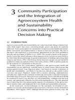
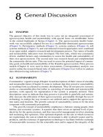
the whole. An overview of such a hierarchical vision of an autocatalytic loop of energy forms
is given in Figure 7.1. This representation can be directly related to the discussion in Chapter
6 about multi-scale mosaic effects for metabolic systems organized in nested hierarchies.
2. It is always possible to adopt multiple legitimate nonequivalent representations of a given
system that are reflecting its ontological characteristics. Therefore, the choice of just one
particular representation among the set of potential representations reflects not only
characteristics of the observed system, but also characteristics of the observer (goals of the
analysis, relevance of system’s qualities included in the semantic identity, credibility of
assumptions about the models, congruence of nonequivalent perceptions of causal relations
in different descriptive domains).
3. A given problem structuring (the system and what it does in its associative context) reflects an
agreement about how to perceive and represent a complex adaptive holarchy in relation to the
choices of (1) a set of semantic identities (what is relevant for the observer about the observed)
and (2) an associated set of formal identities (what can be observed according to available
detectors and measurement schemes), which will be reflected into the selection of variables
used in the model. It is important to notice that such an agreement about what is the system

and what the system is doing in its context is crucial to get into the following step of selection
of formal identities (individuation of variables used as proxies for observable qualities). Prior
to reaching such an agreement about how to structure in scientific terms the problem of how
to represent the system of interest, experimental data do not count as relevant information.
That is, before having a valid (and agreed-upon) problem structuring that will be used to
FIGURE 7.1 Hierarchical levels that should be considered for studying autocatalytic loops of energy forms.
© 2004 by CRC Press LLC
Multi-Scale Integrated Analysis of Agroecosystems174
represent the complex system using different models referring to different scales and different
descriptive domains, data per se do not exist. The possibility of using data requires a previous
validated definition of (1) what should be considered relevant system qualities, (2) which
observable system qualities should be used as proxies of these relevant qualities and (3) what is
the set of measurement schemes that can be used to assign values to the variables, which then
can be used in formal models to represent the system’s behavior. The information provided by
data therefore always reflects the choices made when defining the set of formal identities
adopted in the representation of the reality by the analyst.
Sometimes scientists are aware of the implications of these preanalytical choices, and sometimes they are
not. Actually, the most important reason for introducing complex systems thinking is increasing the
transparency about hidden implications associated with the step of modeling. The approach of impredicative
loop analysis is aimed at addressing this issue. The meat of ILA is about forcing a semantic validity check
over the set of formal identities adopted in the phase of representation by those making models.
To obtain this result, it is necessary to develop meta-models that are able to establish typologies of
relations among parts and wholes, which can be relevant and useful when dealing with a class of
situations. Useful meta-models can be applied, later on, to special (individual) situations belonging to
a given typology. These meta-models, to be useful, have to be based on a standard characterization of
the mechanism of self-entailment among identities of parts, whole and context, defined on different
levels. Actually, this is exactly what is implied by the very concept of impredicative loop. Looking for
meta-models, however, implies accepting the consequence that any impredicative loop does have
multiple possible formalizations. That is, the same procedure for establishing relations among identities
of parts and the whole within a given impredicative loop can be interpreted in different ways by

different analysts, even when applied to the same system considered at the same point in space and
time. Meta-models, by definition, generate families of models based on the adoption of different sets of
congruent formalization of identities. Obviously, at the moment of selecting an experimental design
(or a specific system of accounting), we will have to select just one particular model to be adopted (to
gather experimental data) and stick with it. Experimental work is based on the selection of just one of
the possible formalizations of the meta-model, applied at a specific point in space and time.
This transparent arbitrariness of models that are built in this way should not be considered a weakness
of this approach. On the contrary, in our view, this should be considered a major strength. In fact, after
acknowledging from the beginning the existence of an open space of legitimate options, analysts coming
from different disciplinary backgrounds, cultural contexts or value systems are forced to deal, first of all
and mainly, with the preliminary discussion of semantic aspects associated with the selection of models.
This certainly facilitates a discussion about the usefulness of models and enhances the awareness of crucial
epistemological issues to be considered at the moment of selecting experimental designs.
Below we provide three practical examples of dissipative systems: (1) a preindustrial society of 100
people on a desert island, (2) a comparison of the trajectory of development of two modern societies
that base the metabolism of their economic process on exosomatic energy (Spain and Ecuador), and
(3) the dynamic budget stabilizing the metabolism of terrestrial ecosystems. For the moment, we just
describe how it is possible to establish a relation between characteristics of parts and the whole of these
systems in relation to their associative contexts. Common features of the three analyses will be discussed
in Section 7.3. More general theoretical aspects are discussed in Section 7.5.
7.2.2 Example 1: Endosomatic Societal Metabolism of an Isolated Society on a
Remote Island
7.2.2.1 Goals of the Example—As noted earlier, the ability to keep a dynamic equilibrium between
requirement and supply of energy carriers (e.g., how much food must be eaten vs. how much food can
be produced in a preindustrial society) entails the existence of a biophysical constraint on the relative
sizes and characteristics of various sectors making up such a society. The various activities linked to
both production and consumption must be congruent in terms of an analysis based on a combined use
© 2004 by CRC Press LLC
Impredicative Loop Analysis: Dealing with the Representation of Chicken-Egg Processes 175
of intensive and extensive variables across levels (mosaic effects across levels—Chapter 6). That is, we

can look at the reciprocal entailment among the definitions of size and characteristics of a metabolic
system organized on nested hierarchical levels (parts and whole). Then we can relate it to the aggregate
effect of this interaction on the environment. This is what we call an impredicative loop analysis.
Coming to this first example, we want to make it immediately clear to the reader that the stability
of any particular societal metabolism does not depend only on the ability of establishing a dynamic
equilibrium between requirement and supply of food. The stability of a given human society can be
checked in relation to a lot of other dimensions—i.e., alternative relevant attributes and criteria. For
example, is there enough drinking water? Can the population reproduce in the long term according to
an adequate number of adult males and females? Are the members of the society able to express
coordinated behavior to defend themselves against external attacks? Indeed, using an analysis that
focuses only on the dynamic equilibrium between requirement and supply of food is just one of the
many possible ways for checking the feasibility of a given societal structure.
However, given the general validity of the laws of thermodynamics, such a check cannot be ignored.
As a matter of fact, the same approach (checking the ability of obtaining a dynamic equilibrium
between requirement and supply) can be applied in parallel to different mechanisms of mapping that
can establish forced relations among flows and sizes of compartments and wholes across levels, in
relation to different flows (as already illustrated in Chapter 6), to obtain integrated analysis. The reader
can recall here the example of the various medical tests to be used in parallel to check the health of a
patient (Figure 6.3). In this first example of impredicative loop analysis we will look at the dynamic
budget of food energy for a society. This is like if we were looking at the bones—using x-rays—of our
patient. Other types of impredicative loop analysis (next two examples) could represent nonequivalent
medical tests looking at different aspects of the patient (e.g., ultrasound scan and blood test). What is
important is to have the possibility, later on, to have an overview of the various tests referring to
nonequivalent and nonreducible dimensions of performance. This is done, for example, in Figure 7.6,
which should be considered an analogous to Figure 6.3.
7.2.2.2 The Example—As soon as we undertake an analysis based on energy accounting, we have to
recognize that the stabilization of societal metabolism requires the existence of an autocatalytic loop of
useful energy (the output of useful energy is used to stabilize the input). In this example, we characterize the
autocatalytic loop stabilizing societal metabolism in terms of reciprocal entailment of the two resources:
human activity and food (Giampietro, 1997). The term autocatalytic loop indicates a positive feedback, a self-

reinforcing chain of effects (the establishment of an egg-chicken pattern). Within a socioeconomic process
we can define the autocatalytic loop as follows: (1) The resource human activity is needed to provide control
over the various flows of useful energy (various economic activities in both producing and consuming),
which guarantee the proper operation of the economic process (at the societal level). (2) The resource food
is needed to provide favorable conditions for the process of reproduction of the resource human activity
(i.e., to stabilize the metabolism of human societies when considering elements at the household level). (3)
The two resources, therefore, enhance each other in a chicken-egg pattern. In this example we are studying
the possibility of using the impredicative loop analysis related to the self-entailment of identities of parts and
the whole, which are responsible for stabilizing the autocatalytic loop of two energy forms: chemical energy
in the food and human activity expressed in terms of muscle and brain power.
Within this framework our heuristic approach has the goal of establishing a relation between a
particular set of parameters determining the characteristics of this autocatalytic loop as a whole (at
level n) and a particular set of parameters that can be used to describe the characteristics of the various
elements of the socioeconomic system at a lower level (level n-1). These characteristics can be used to
establish a bridge with technological changes (observed on the interface of level n-1/level n-2) and to
effect changes on environmental impact at the interface—level n/level n+1 (see Figure 7.1).
In this simplified example, we deal with an endosomatic autocatalytic loop (only human labor and
food) referring to a hypothetical society of 100 people on an isolated, remote island. The numbers
given in this example per se are not the relevant part of the analysis. As noted earlier, no data set is
relevant without a previous agreement of the users of the data set about the relevance of the problem
© 2004 by CRC Press LLC
Multi-Scale Integrated Analysis of Agroecosystems176
structuring (in relation to a specific analysis performed in a specific context). We are providing numbers—
which are familiar for those dealing with this topic—just to help the reader to better grasp the mechanism
of accounting. It is the forced relation among numbers (and the analysis of the mechanism generating
this relation) that is the main issue here. Different analysts can decide to define the relations among the
parts and the whole in different ways, and therefore this could lead to a different definition of the data
set. However, when adopting this approach, they will be asked by other analysts about the reasons for
their different choices. This then will require discussing the meaning of the analysis.
The following example of ILA presenting a useful metaphor (meta-model) for studying societal

metabolism has two major goals:
1. To illustrate an approach that makes it possible to establish a clear link between the characteristics
of the societal metabolism as a whole (characteristics referring to the entire loop—level n) and
a set of parameters controlling various steps of this loop (characteristics referring to lower-
level elements and higher-level elements—defined at either level n-1 or level n+ 1). Moreover,
it should be noted that the parameters considered in this analysis are those generally considered,
by default, as relevant in the discussion about sustainability (e.g., population pressure, material
standard of living, technology, environmental loading). This example clearly shows that these
parameters are actually those crucial in determining the feasibility of the autocatalytic loop,
when characterized in terms of impredicative loop analysis.
2. To illustrate the importance of closing the loop when describing societal metabolism in energy
terms, instead of using linear representations of energy flows in the economic process (as done
with input/output analyses). In fact, the conventional approach usually adopted in energy
analysis, based on conventional wisdom, keeps its focus on the consideration of a unidirectional
flow of energy from sources to sinks (the gospel says “while matter can be recycled over and
over, energy can flow only once and in one direction”). As discussed in Section 7.4, a linear
representation of energy flows in terms of input/output assessments cannot catch the reciprocal
effect across levels and scales that the process of energy dissipation implies (Giampietro and
Pimentel, 1991a; Giampietro et al., 1997). In fact, it is well known that in complex adaptive
systems, the dissipation of useful energy must imply a feedback, which tends to enhance the
adaptability of the system of control (Odum, 1971, 1983, 1996). Assessing the effect of such
feedback, however, is not simple because this feedback can only be detected and represented
on a descriptive domain that is different (larger space-time scale) from the one used to assess
inputs, outputs and flows (as discussed at length in Sections 7.4 and 7.5). This is what
GeorgescuRoegen (1971) describes as the impossibility to perform an analytical representation
of an economic process when several distinct time differentials are required in the same analytical
domain. Actually, he talks of the existence of incompatible definitions of duration for parallel
input/output processes (the replacement of the term duration with the term time differentials is
ours). Our ILA of the 100 people on the remote island provides practical examples of this fact.
The representations given in Figure 6.6 of how endosomatic energy flows in a society is a classic example

of the conventional linear view. Energy flows are described as unidirectional flows from left to right (from
primary sources to end uses). However, it is easy to note that some of the end uses of energy (indicated on
the right side) are necessary for obtaining the input of energy from primary energy sources (indicated on
the left side) in the first place. That is, the stabilization of a given societal metabolism is linked to the ability
to establish an egg-chicken pattern within flows of energy. In practical terms, when dealing with the
endosomatic metabolism of a human society, a certain fraction of end uses (e.g., in Figure 6.6, the physical
activity “work for food”) must be available and used to produce food. The expression autocatalytic loop
actually indicates the obvious fact that some of the end uses must reenter into the system as input to
sustain the overall metabolism. This is what implies the existence of internal constraints on possible
structures of socioeconomic systems. In practical terms, when dealing with the endosomatic metabolism
of a human society, a certain fraction of the end uses must be available and used to produce food before
the input enters into the system (as indicated on the lower axis of Figure 7.2).
© 2004 by CRC Press LLC
Impredicative Loop Analysis: Dealing with the Representation of Chicken-Egg Processes 177
7.2.2.3 Assumptions and Numerical Data for This Example—We hypothesize that a society of
100 people uses only flows of endosomatic energy (food and human labor) for stabilizing its own
metabolism. To further simplify the analysis, we imagine that the society is operating on a remote island
(survivors of a plane crash). We further imagine that its population structure reflects the one typical of
a developed country and that the islanders have adopted the same social rules regulating access to the
workforce as those enforced in most developed countries (that is, persons under 16 and those over 65
are not supposed to work). This implies a dependency ratio of about 50%; that is, only 50 adults are
involved in the production of goods and social services for the whole population. We finally add a few
additional parameters needed to characterize societal metabolism. At this point the forced loop in the
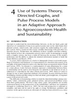
relation between these numerical values is described in Figure 7.2:
• Basic requirement of food. Using standard characteristics of a population typical of
developed countries, we obtain an average demand of 9 MJ/day/capita of food, which
translates into 330,000 MJ/year of food for the entire population.
• Indicator of material standard of living. We assume that the only “good” produced and
consumed in this society (without market transactions) is food providing nutrients to the
diet. In relation to this assumption we can then define two possible levels of material standard

of living, related to two different qualities for the diet. The two possible diets are: (1) Diet A,
which covers the total requirement of food energy (3300 MJ/year/capita) using only cereal
(supply of only vegetal proteins). With a nutritional value of 14 MJ of energy/kg of cereal,
this implies the need to produce 250 kg of cereal/year/capita. (2) Diet B, which covers 80%
of the requirement of food energy with cereal (190 kg/year per capita (p.c.)) and 20% with
beef (equivalent to 6.9 kg of meat/year p.c.). Due to the very high losses of conversion (to
produce 1 kg of beef you have to feed the herd 12 kg of grain), this double conversion
implies the additional production of 810 kg of cereal/year. That is, Diet B requires the
primary production of 1000 kg of cereal/capita (rather than 250 kg/year of Diet A). Actually,
the value of 1000 kg of cereal consumed per capita, in indirect form in the food system, is
exactly the value found in the U.S. today (see the relative assessment in Figure 3.1).
FIGURE 7.2 One hundred people on a remote island.
© 2004 by CRC Press LLC
Multi-Scale Integrated Analysis of Agroecosystems178
• Indicator of technology. This reflects technological coefficients, in this case, labor productivity
and land productivity of cereal production. Without external inputs to boost the production,
these are assumed to be 1000 kg of cereal/hectare and 1 kg of cereal/hour of labor.
• Indicator of environmental loading. A very coarse indicator of environmental loading
can be assessed by the fraction land in production/total land of the island, since the land
used for producing cereal implies the destruction of natural habitat (replaced with the
monoculture of cereal). In our example the indicator of environmental loading is heavily
affected by the type of diet followed by the population (material standard of living) and the
technology used. Assuming a total area for the island of 500 ha, we have an index of EL=0.05
for Diet A and EL=0.20 for Diet B (EL=hectares in production/total hectares available on
the island).
• Supply of the resource human activity. We imagine that the required amount of food
energy for a year (330,000 MJ/year) is available for the 100 people for the first year (assume
it was in the plane). With this assumption, and having the 100 people to start with, the
conversion of this food into endosomatic energy implies (it is equivalent to) the availability
of a total supply of human activity of 876,000 h/year (24 h/day×365×100 persons).

• Profile of investment of human activity of a set of typologies of end uses of
human activity (as in Figure 7.2). These are:
1. Maintenance and reproduction—It should be noted that in any human society the largest
part of human activity is not related to the stabilization of the societal metabolism (e.g.,
in this case producing food), but rather to maintenance and reproduction of humans.
This fixed overhead includes:
a. Sleeping and personal care for everybody (in our example, a flat value of 10 h/day has
been applied to all 100 people, leading to a consumption of 365,000 h/year of the
total human activity available).
b. Activity of nonworking population (the remaining 14 h/day of elderly and children,
which are important for the future stability of the society, but which are not
available—according to the social rule established before—for the production of
food). This indicates the consumption of another 255,000 h/year (14×50×365) in
nonproductive activities.
2. Available human activity for work—The difference between total supply of human activity
(876,000 h) and the consumption related to the end use maintenance and reproduction
(620,000 h) is the amount of available human activity for societal self-organization (in
our example, 256,000 h/year). This is the budget of human activity available for stabilizing
societal metabolism. However, this budget of human activity, expressed at the societal
level, has to be divided between two tasks:
a. Guaranteeing the production of the required food input (to avoid starvation)—work
for food
b. Guaranteeing the functioning of a good system of control able to provide adaptability
in the future and a better quality of life to the people—social and leisure
At this point, the circular structure of the flows in Figure 7.2 enters into play. The requirement of
330,000 MJ/year of endosomatic energy input (food at time t) entails the requirement of producing
enough energy carriers (food at time t+1) in the following years. That is a biophysical constraint on the
level of productivity of labor in the activity producing food. Therefore, this characteristic of the whole
(the total demand of the society) translates into a nonnegotiable fraction of investment of available
human activity in the end use work for food (depending on technology and availability of natural

resources). This implies that the disposable fraction of available human activity, which can be allocated
to the end use social and leisure, is not a number that can be decided only according to social or
political will. The circular nature of the autocatalytic loop implies that numerical values associated with
the characterization of various identities defining elements on different hierarchical levels (at the level
of individual compartments; extensive—segments on the axis—and intensive variables; wideness of
angles) can be changed, but only respecting the constraint of congruence among flows over the whole
© 2004 by CRC Press LLC
Impredicative Loop Analysis: Dealing with the Representation of Chicken-Egg Processes 179
loop. These constraints are imposed on each other by the characteristics and size—extensive (1 and 2)
and intensive (3) variables—of the various compartments.
7.2.2.4 Changing the Value of Variables within Formal Identities within a Given
Impredicative Loop —Imagine to change, for example, some of the values used to characterize
this autocatalytic loop of energy forms. For example, let us change the parameter “material standard of
living,” which in our simplified model is expressed by a formal definition of quality of the diet. The
different mix of energy vectors in the two diets (vegetal vs. animal proteins) implies a quantitative
difference in the biophysical cost of the diet expressed in terms of both a larger work requirement and
a larger environmental loading (higher demand of land). The production of cereal for a population
relying 100% on Diet A requires only 25,000 h of labor and the destruction of 25 ha of natural habitat
(EL
A
=0.05), whereas the production of cereal for a population relying 100% on Diet B requires 100,000
h of labor and the destruction of 100 ha of natural habitat (EL
B
=0.20). However, to this work quantity
required for producing the agricultural crop, we have to add a requirement of work for fixed chores.
Fixed chores are preparation of meals, gathering of wood for cooking, getting water, and washing and
maintenance of food system infrastructures in the primitive society. In this example we use the same
flat value for the two diets—73,000 h/year (2 h/day/capita=2×365×100). This implies that if all the
people of the island decide to follow Diet A, they will face a fixed requirement of “work for food” of
98,000 h/year. If they all decide to adopt Diet B, they will face a fixed requirement of “work for food”

of 173,000 h/year. At this point, for the two options we can calculate the amount of disposable available
human activity that can be allocated to social and leisure. It is evident that the amount of time that the
people living in our island can dedicate to running social institutions and structures (schools, hospitals,
courts of justice) and developing their individual potentialities in their leisure time in social interactions
is not the result of their free choice. Rather, it is the result of a compromise between competing
requirements of the resource “available human activity” in different parts of the economic process.
That is, after assigning numerical values to social parameters such as population structure and a
dependency ratio for our hypothetical population, we have a total demand of food energy (330,000 MJ/
year) and a fixed overhead on the total supply of human activity, which implies a flat consumption for
maintenance and reproduction (620,000 h/year). Assigning numerical values to other parameters, such as
material standard of living (Diet A or Diet B) and technical coefficients in production (e.g., labor, land and
water requirements for generating the required mix of energy vectors), implies defining additional constraints
on the feasibility of such a socioeconomic structure. These constraints take the form of (1) a fixed requirement
of the resource “available human activity” that is absorbed by “work for food” (98,000 h for Diet A and
173,000 h for Diet B) and (2) a certain level of environmental loading (the requirement of land and water,
as well as the possible generation of wastes linked to the production), which can be linked, using technical
coefficients, to such a metabolism (in our simple example we adopted a very coarse formal definition of
identity for environmental loading that translates into EL
A
= 0.05 and EL
B
=0.20).
With the term internal biophysical constraints we want to indicate the obvious fact that the amount of
human activity that can be invested into the end uses “maintenance and reproduction” and “social and
leisure” depends only in part on the aspirations of the 100 people for a better quality of life in such a
society. The survival of the whole system in the short term (the matching of the requirement of energy
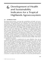
carriers’ input with an adequate supply of them) can imply forced choices (Figure 7.3). Depending on
the characteristics of the autocatalytic loop, large investments of human activity in social and leisure
can become a luxury. For example, if the entire society (with the set of characteristics specified above)
wants to adopt Diet B, then for them it will not be possible to invest more than 83,000 h of human

activity in the end use “social and leisure.” On the other hand, if they want, together with a good diet,
also a level of services typical of developed countries (requiring around 160,000 h/year/100 people),
they will have to “pay” for that. This could imply resorting to some politically important rules reflecting
cultural identity and ethical believes (what is determining the fixed overhead for maintenance and
reproduction). For example, to reach a new situation of congruence, they could decide to either
introduce child labor or increase the workload for the economically active population (e.g., working
10 h a day for 6 days a week) (Figure 7.3). Alternatively, they can accept a certain degree of inequity in
© 2004 by CRC Press LLC
Multi-Scale Integrated Analysis of Agroecosystems180
the society (a small fraction of people in the ruling social class eating Diet B and a majority of the ruled
eating Diet A). We can easily recognize that all these solutions are today operating in many developing
countries and were adopted, in the past, all over our planet.
7.2.2.5 Lessons from This Simple Example—The simple assumptions used in this example for bringing
into congruence the various assessments related to a dynamic budget of societal metabolism are of course
not realistic (e.g., nobody can eat only cereal in one’s diet, and expected changes in the requirements of
work are never linear). Moreover, by ignoring exosomatic energy, we do not take in account the effect of
capital accumulation (e.g., potential use of animals, infrastructures, better technology and know-how
affecting technical coefficients), which is relevant for reaching new feasible dynamic points of equilibrium
of the endosomatic energy budget. That is, alternative points of equilibrium can be reached by, besides
changing population structure and size, changing technology (and the quality of natural resources). Actually,
it is easy to make models for preindustrial societies that are much more sophisticated than the one
presented in Figure 7.2: models that take into account different landscape uses, detailed profiles of human
time use, and reciprocal effects of changes on the various parameters, such as the size and age distribution
of society (Giampietro et al., 1993). These models, after entering real data derived from specific case
studies, can be used for simulations, exploring viability domains and the reciprocal constraining of the
various parameters used to characterize the endosomatic autocatalytic loop of these societies. However,
models dealing only with the biophysical representation of endosomatic metabolism and exosomatic
conversions of energy are not able to address the economic dimension. Economic variables reflect the
expression of human preferences within a given institutional setting (e.g., an operating market in a given
context) and therefore are logically independent from assessment reflecting biophysical transformations.

Even within this limitation, the example of the remote island clearly shows the possibility of linking
the representation of the conditions determining the feasibility of the dynamic energy budget of
societal metabolism to a set of key parameters used in the sustainability discussions. In particular,
FIGURE 7.3 One hundred people on a remote island.
© 2004 by CRC Press LLC
Impredicative Loop Analysis: Dealing with the Representation of Chicken-Egg Processes 181
characterizing societal metabolism in terms of autocatalytic loops makes it possible to establish relations
among changes occurring in parallel in various parameters, which are reflecting patterns perceived on
different levels and scales. For example, how much would the demand of land change if we change the
definition of the diet? How much would the disposable available human activity change if we change
the dependency ratio (by changing population structure or retirement age)? In this way, we can explore
the viability domain of such a dynamic budget (what combination of values of parameters are not
feasible according to the reciprocal constraints imposed by the other parameters).
and Figure 7.3 in terms of potential changes in characteristics (e.g., either the values of numbers on
axis or the values of angles) requires using in parallel trend analysis on nonequivalent descriptive
domains. In fact, changes that are affecting the value taken by angles (intensive variables) or the length
of segments on axes (extensive variables) require considering nonequivalent dynamics of evolutions
reflecting different perceptions and representations of the system. These relations are those considered
in the discussion about mosaic effect across levels in Chapter 6.
For example, if the population pressure and the geography of the island imply that the requirement
of 100 ha of arable land are not available for producing 100,000 kg of cereal (e.g., a large part of the 500
ha of the island is too hilly), the adoption of Diet B by 100% of the population is simply not possible.
The geographic characteristics of the island (defined at level n+2) can be, in this way, related to the
characteristics of the diet of individual members of the society (at level n-2). This relation between
shortage of land and poverty of the diet is well known. This is why, for example, all crowded countries
depending heavily on the autocatalytic loop of endosomatic energy for their metabolism (such as India
or China) tend to have a vegetarian diet. Still, it is not easy to define such a relation when adopting just
one of these nonequivalent descriptive domains.
To make another hypothesis of perturbation within the ILA shown in Figure 7.2, imagine the
arrival of another crashing plane with 100 children on board (or a sudden baby boom on the island).

This perturbation translates into a dramatic increase of the dependency ratio. That is, a higher food
demand, for the new population of 200 people would have to be produced by the same amount of
256,000 h of available human activity (related to the same 50 working adults). In this case, even when
adopting Diet A, the larger demand of work in production will force such a society to dramatically
reduce the consumption of human activity in the end use related to social and leisure. The 158,000 h/
year, which were available to a society of 100 vegetarians (adopting 100% Diet A) for this end use—
before the crash of the plane full of children—can no longer be afforded. This could imply that the
society would be forced to reduce the investments of human activity in schools and hospitals (to be
able to produce more food), at the very moment in which these services should be dramatically
increased (to provide more care to the larger fraction of children in the population). This could appear
as uncivilized behavior to an external observer (e.g., a volunteer willing to save the world in a poor
marginal area of a developing country). This value judgment, however, can only be explained by the
ignorance of such an external observer of the existence of biophysical constraints that are affecting the
very survival of that society. Survival, in general, gets a higher priority than education.
The information used to characterize the impredicative loop that is determining the societal metabolism
of a society translates into an organization of an integrated set of constraints over the value that can be
taken by a set of variables (both extensive and intensive). In this way, we can facilitate the discussion and
evaluation of possible alternative solutions for a given dynamic budget in terms of trade-off profiles. We
earlier defined sustainability as a concept related to social acceptability, ecological compatibility, stability
of social institutions, and technical and economic feasibility. Even when remaining within the limits of
this simple example, we can see the integrative power of this type of multi-level integrated analysis. In
fact, the congruence among the various numerical values taken by parameters characterizing the
autocatalytic loop of food can be obtained by using different combinations of numerical values of variables
defined at different hierarchical levels and reflecting different dimensions of performance. There are
variables or parameters (e.g., technical coefficients) that refer to a very location-specific space-time scale
(the yield of cereal at the plot level in a given year) and others (e.g., dependency ratio) that reflect
biophysical processes (demographic changes) with a time horizon of changes of 20 years. Finally, there are
© 2004 by CRC Press LLC
A technical discussion of the sustainability of the dynamic energy budget represented in Figure 7.2
Multi-Scale Integrated Analysis of Agroecosystems182

other variables or parameters (e.g., regulation imposed for ethical reasons, such as compulsory school for
children) that reflect processes related to the specific cultural identity of a society.
For example, data used so far in this example about the budget of the resource human activity (for 100
people) reflect standard conditions found in developed countries (50% of the population economically
active, working for 40 h/week×47 weeks/year). Now imagine that for political reasons we are introducing
a working week of 35 h (keeping five or six weeks of vacation per year)—a popular idea nowadays in
Europe. Comparing this new value to previous workload levels, this implies moving from about 1800 to
about 1600 h/year/active worker (work absences will further affect both). This reduction is possible only
if this new value is congruent with the requirement imposed by technical coefficients (the requirement
of work for food) and the existing level of investments/consumption in the end use “maintenance and
reproduction.” If this is not the case, depending on how strong is the political will of reducing the number
of hours per week, the society has the option of altering some of the other parameters to obtain a new
congruence. One can decide to increase the retirement age (by reducing the consumption of human
activity by “maintenance and reproduction,” that is, by reducing the amount of nonworking human
activity associated with the presence of elderly in the population) or to decrease the minimum age
required for entering the workforce (a very popular solution in developing countries, where children
below 16 years generally work). Another solution could be that of looking for better technical coefficients
(e.g., producing more kilograms of cereal per hour of labor), but this would require both a lag time to get
technical innovations and an increase in investments of human work in research and development.
Actually, looking for better technical coefficients is the standard solution to all kinds of dilemmas
about sustainability looked for in developed countries (since this makes it possible to avoid facing conflicts
internal to the holarchy). This is what we called in Part 1 the search for silver bullets or win-win-win
solutions. However, any solution based on the adding of more technology does not come without side
effects. It requires adjustments all over the impredicative loop. Moreover, this solution could imply an
increase in the environmental impact of societal metabolism (e.g., in our example, increasing the
performance of monocultures could increase the environmental impact on the ecosystem of the island).
Again, when we frame the discussion of these various options within the framework of integrated analysis
of societal metabolism over an impredicative loop, we force the various analysts to consider, at the same
time, several distinct effects (nonequivalent models and variables) belonging to different descriptive domains.
To make things more difficult, the consideration in parallel of different levels and scales can imply

reversing the direction of causation in our explanations. That is, the direction of causality will depend on
what we consider to be the independent definitions of identity (parameters) and the dependent definitions
of identities (variables) within the impredicative loop (Figure 7.4). For example, looking at the four
quadrants shown in Figure 7.4, we see that physiological characteristics (e.g., average body mass) can be
given (e.g., in the example of the plane full of Western people crashing on the island, we are dealing with
an average body mass of more than 65 kg for adults). On the other hand, if the average body mass is
considered a dependent variable (e.g., in the long term, when adopting the hypothesis of “small and
healthy” physiological adaptation to reduce food supply), we can expect that, as occurring in preindustrial
societies, in the future we will find on this island adults with a much smaller average body mass. In the
same way, the demographic structure can be a variable (when importing only adult immigrants, whenever
a larger fraction of workforce is required) or a given constraint (when operating in a social system where
emigration or immigration are not an option). The same applies to social rules (e.g., slavery can be
abolished and declared immoral when no longer needed or used to boost the performance of the economy
and the material standard of living of the masters). In the same way, what should be considered an
acceptable level of service is another system quality that can be considered a dependent variable (e.g., if
you are in a marginal social group forced to accept whatever is imposed on you) by the system. It
becomes an independent variable, though, for groups that have the option to force their governments to
do better or that have the option to emigrate. Technical coefficients can be seen as driving changes in
other system qualities, when adopting a given timescale (e.g., population grew because better technology
made available a larger food supply), or they can be seen as driven by changes in other system qualities
when adopting another timescale (e.g., technology changed because population growth required a larger
food supply). Every time the analyst decides to adopt a given formalization of this impredicative loop
© 2004 by CRC Press LLC
Impredicative Loop Analysis: Dealing with the Representation of Chicken-Egg Processes 183
based on a preanalytical definition of what is a parameter and what is a variable (which in turn implies
choosing a given triadic filtering on the perception of the reality), such a decision implies exploring
the nature of a certain mechanism (and dynamics) by ignoring the nature of others. Recall the different
explanations for the death of a person (Figure 3.5) or the example of the plague in the village in
Tanzania (Figure 3.6).
This fact, in our view, is crucial, and this is why we believe that a more heuristic approach to multi-

scale integrated analysis is required. Reductionist scientists use models and variables that are usually
developed in distinct disciplinary fields. These reductionist models can deal only with one causal
mechanism and one optimizing function at a time, and to be able to do so, they bring with them a lot
of ideological baggage very often not declared to the final users of the models.
We believe that by adopting impredicative loop analysis we can enlarge the set of analytical tools
that can be used to check nonequivalent constraints (lack of compatibility with economic, ecological,
technical and social processes), which can affect the viability of considered scenarios. This approach can
be used to generate a flexible tool bag for making checks based on different disciplinary knowledge,
while keeping at the same time an approach that guarantees congruence among the various assessments
referring to nonequivalent descriptive domains (some formal check on congruence among scenarios).
7.2.3 Example 2: Modern Societies Based on Exosomatic Energy
Impredicative loop analysis applied to self-entailment among the set of identities—energy carriers
(level n-2); converters used by components (on the interface level n-2/level n-1); the whole seen as a
network of parts (on the interface level n-1/level n); and the whole seen as a black box interacting with
its context (on the interface level n/level n+1)—is required to represent the metabolism of exosomatic
energy in modern societies, as illustrated in Figure 7.1. The way to deal with such a task is illustrated in
Figure 7.5 (more details in theoretical Section 7.4). The four angles refer to the forced congruence
among two different forms of energy flowing in the socioeconomic process: (1) fossil energy used to
power exosomatic devices, which is determining/determined by (2) human activity used to control
the operation of exosomatic devices. For more on this rationale, see Giampietro (1997).
There two sets of four-angle figures that are shown in Figure 7.5. Two of these four-angle figures (small
around the origin of axes) represent two formalizations of the impredicative loop generating the energy budget
of Ecuador at two points in time (1976 and 1996). The other two four-angle figures (dotted and solid squares)
FIGURE 7.4 Arbitrariness associated with a choice of a time differential.
© 2004 by CRC Press LLC
Multi-Scale Integrated Analysis of Agroecosystems184
represent two formalizations of the impredicative loop generating the energy budget of Spain at the same
two points in time: 1976 and 1996. This figure clearly shows that by adopting this approach, it is possible
to address the issue of the relation between qualitative changes (related to the readjustment of reciprocal
values of intensive variables within a given whole) and quantitative changes (related to the values taken by

extensive variables—that is, the change in the size of internal compartments and the change of the system
as a whole). The approach used to draw Figure 7.5 is basically the same as that used in Figure 7.2 in terms
of the basic rationale. That is, the set of activities required for food production within the autocatalytic
loop of endosomatic energy has been translated into the set of activities producing the required input of
useful energy for machines (energy and mining+manufacturing).
For a more detailed explanation of the formalization used in the four-angle figures shown in Figure
7.5, see Giampietro (1997), Giampietro et al. (2001) and the two special issues of Population and
Environment (Vol. 22, pp. 97–254, 2000; and Vol. 22, pp. 257–352, 2001). Moreover, a detailed explanation
of this type of analysis will be discussed in Chapter 9 when discussing the concepts of demographic
and socioeconomic pressure on agricultural production.
Economic growth is often associated with an increase in the total throughput of societal metabolism,
and therefore with an increase in the size of the whole system (when seen as a black box). However, when
studying the impredicative loop that is determining an integrated set of changes in the relative identities
of different elements (e.g., economic sectors seen as the parts) and the whole, we can better understand
the nature and effects of these changes. That is, the mechanism of self-entailment of the possible values
taken by the angles (intensive variables) reflects the existence of constraints on the possible profiles of
distribution of the total throughput over lower-level compartments. In the example given in Figure 7.5,
Spain changed, over the considered period, the characteristics of its metabolism both in (1) qualitative
terms (development—different profile of distribution of the throughput over the internal compartments;
changes in the value taken by intensive 3 variables, i.e., angles) and (2) quantitative terms (growth—
increase in the total throughput; changes in the value taken by extensive variables, i.e., segments).
On the other hand, Ecuador, in the same period, basically expanded only the size of its metabolism
(the throughput increased as a result of an increase in redundancy—more of the same; increase in
FIGURE 7.5 Total human activity.
© 2004 by CRC Press LLC
Impredicative Loop Analysis: Dealing with the Representation of Chicken-Egg Processes 185
extensive variable 2, i.e., segments), but maintained the original relation among intensive variables (the
same profile of distribution of values of intensive variables 3, i.e., angles reflecting the characteristics of
lower-level components; growth without development). In our view, an analytical approach based on
an impredicative loop analysis can provide a powerful diagnostic tool when dealing with issues related

to sustainability, environmental impact associated with growth and development (e.g., when dealing
with issues such as the mythological environmental Kuznet curves). In fact, in these situations it is very
easy to extrapolate wrong conclusions (e.g., dematerialization of developed economies) after being
misguided by the reciprocal effect of changes among intensive and extensive variables—Jevons’ paradox
(see Figure 1.3)—leading to the generation of treadmills, as discussed in Table 1.1.
7.2.4 Example 3: The Net Primary Productivity of Terrestrial Ecosystems
7.2.4.1 The Crucial Role of Water Flow in Shaping the Identity of Terrestrial Ecosystems
Before getting into the discussion of the next example of ILA applied to the mechanism of self-
entailment of energy forms associated with the identity of different types of terrestrial ecosystems, it is
useful to quote an important passage of Tim Allen about the crucial role of water in determining the
life of terrestrial ecosystems:
Living systems are all colloidal and, for the narrative we wish to tell, water is the constraining
matrix wherein all life functions. Unfortunately, most biological discussion turns on issues of
carbon chemistry, such as photosynthesis, and the water is taken for granted. Think then of the
amount of water that is in your head as you think about these ideas. Your thoughts are held in
a brain that is over 80% water. Might it not be foolish to take that water for granted. Water is
the medium in which life is constrained. Mars is a dead planet because it has insufficient
liquid water. The controls of Gaia (Lovelock, 1986) on this planet work through water as a
medium of operation. There is no life on Mars because there is no water to get organized.
When we take water seriously, as a matrix of life, living systems are an emergent property not
of carbon and its chemistry, but an emergent property of planetary water. Thus I misspeak
when I tell my students that terrestrial animals are zooplankton that have brought their water
with them. Rather they are pieces of ocean water that has brought its zooplankton with it. In
the time between the next to last breath of a dying organisms and when it is unequivocally
death, the carbon chemicals within the corps are essentially unchanged. The difference between
life and death is that the water ceases to be the constraining element and it leaks away. The
water loses its control. Trees are one of water’s ways of getting around on land and into the air
(Allen et al., 2001, p. 136).
This passage beautifully focuses on the crucial importance of water and the role that it (and its activity
driven by dissipation of energy) plays in the functioning of terrestrial ecosystems. From this perspective,

one can appreciate that the net primary productivity (NPP) of terrestrial ecosystems (the ability to use
solar energy in photosynthesis to make chemical bonds) depends on the availability of a flow of energy
of different natures (the ability to discharge entropy to the outer space, associated with the
evapotranspiration of water). That is, the primary productivity of terrestrial ecosystems, which establishes
a store of free energy in the form of chemical bonds in standing biomass, requires the availability of a
different form of energy at a higher level. According to the seminal concept developed by Tsuchida,
the identity of Gaia is guaranteed by an engine powered by the water cycle that is able to discharge
entropy at an increasing rate (see Tsuchida and Murota, 1985). This power is required to stabilize
favorable boundary conditions of the various terrestrial ecosystems operating on the planet.
When coming to agricultural production in agroecosystems, the situation is even more complicated.
In fact, to have agricultural production, additional types of energy forms and conversions are required.
At least three distinct types of energy flows (each of which implies a nonequivalent definition of
identities for converters, components, wholes and admissible environments) are required for the stability
of an agroecosystem:
© 2004 by CRC Press LLC
Multi-Scale Integrated Analysis of Agroecosystems186
1. Natural processes of energy conversions powered by the sun and totally out of
human control. These can include, for example, heat transfer due to direct radiation,
evapotranspiration of water, generation of chemical bonds via photosynthesis and interactions
of organisms belonging to different species within a given community to stabilize existing
food webs (i.e., for the reciprocal control predator-prey or plants-herbivores-carnivores-
detritus feeders within nutrient loops in ecosystems).
2. Natural processes of conversion of food energy within humans and domesticated
plants and animals controlled by humans to generate useful power. This metabolic
energy is used to generate human work and animal power needed in farming activities, as
well as plants and animal products (such as crops, fibers, meat, milk and eggs).
3. Technology-driven conversions of fossil energy (these conversions require the availability
of technological devices—capital—and know-how, besides the availability of fossil energy
stocks). Fossil energy inputs are used to boost the productivity of land and labor (e.g., for
irrigation, fertilization, pest control, tilling of soil, harvesting). This input to agriculture is

coming from stock depletion (mining of fossil energy deposits) and therefore implies a
dangerous dependency of food security on nonrenewable resources.
These three types of energy flows have a different nature and therefore cannot be described within the
same descriptive domain (not only the relative patterns are defined on nonreducible descriptive domains,
but also their relative sizes, are too different). Therefore, it is important to be able to establish at least
some sort of bridge among them. An integrated assessment has to deal with all of them, since they are
required in parallel—and in the right range of values, intensive variable 3—for sustaining a stable flow
of agricultural production.
Relevant implications of this fact are:
1. When describing the process of agricultural production in terms of output/input energy
ratios (using conventional energy analyses), the analyst tends to basically focus only on those
activities and energy flows that have direct importance (in terms of costs and benefits) for
humans. That is, the traditional accounting of output/input energy ratios in agricultural
production refers to outputs directly used by humans (e.g., harvested biomass and useful by-
products) and inputs directly provided by humans (e.g., application of fertilizers, irrigation,
tilling of soil). That is, such an accounting refers to a perception of usefulness obtained from
within the socioeconomic system (from within the black box). However, these two flows do
not necessarily have to be relevant for the perspective of the ecosystem in which the agricultural
production takes place. Actually, it should be noted that the two flows of energy considered in
conventional energy assessments as input and output of the agricultural production are only a
negligible fraction of the energy flowing in any agroecosystem. Any biomass production (both
controlled by humans and naturally occurring) requires a very large amount of solar energy to
keep favorable conditions for the process of self-organization of plants and animals. There are
large-scale ecological processes occurring outside human control that are affecting both the
supply of inputs and the stability of favorable boundary conditions to the process of agricultural
production. That is, what is useful to stabilize the set of favorable conditions required by
primary production of biomass in terrestrial ecosystems—the flow of useful activity of ecological
processes—can be perceived and represented only by adopting a triadic reading of events on
higher levels (level n, n+1, or n+2). This is a triadic reading different from that adopted to
represent the process of agricultural production at the farm level (level n-1, n, or n+1). These

mechanisms operating at higher levels are totally irrelevant in terms of short-term perception
of utility for humans and tend not to be included in assessments based on monetary variables.
A tentative list of ecological services required for the stability of primary productivity of
terrestrial ecosystems and ignored by default by monetary accounting include (1) an adequate
air temperature, (2) an adequate inflow of solar radiation, (3) an adequate supply of water and
nutrients, (4) healthy soil that makes the available water and nutrients accessible to plants at the
© 2004 by CRC Press LLC
Impredicative Loop Analysis: Dealing with the Representation of Chicken-Egg Processes 187
right moment and (5) the presence of useful biota able to guarantee the various steps of
reproductive cycles (e.g., seeds, insects for pollination).
2. The two flows of energy considered in conventional energy assessments as input and output
of the agricultural production are referring to energy forms that require the use of different
sets of identities for their assessment. The majority of energy inputs in modern agriculture
belong to the type fossil energy used in converters, which in general are machines (what we
before called exosomatic energy). The majority of energy output consists of the produced
biomass, which belongs to the type food energy used in physiological converters (what we
before called endosomatic energy). Therefore, this is a ratio between numbers that are reflecting
logically independent assessments (they refer to two different autocatalytic loops of energy
forms, as discussed in the two previous examples). This ratio divides apples by oranges—an
operation that can be legitimately done to calculate indicators (e.g., dependency of food
supply on disappearing stocks of fossil energy) or to benchmark (comparing environmental
loading, or capital intensities of two systems of production), but not to study indices of
performance about evolutionary trajectories of metabolic systems.
Just to provide an idea of the crucial dependency of the human food supply on the stability of existing
biogeochemical cycles on this planet, it is helpful to use a few figures. The total amount of exosomatic
energy controlled by humankind in 1999, for all its activities (agriculture, industry, transportation,
military activities and residential), is around 11 TW (1 TW=10
12
J/sec), which is about 350×10
18

J/year
(BP-Amoco, 1999). For keeping just the water cycle, the natural processes of Earth are using 44,000
TW of solar energy (about 1,400,000×10
18
J/year), 4000 times the energy under human control.
Coming to assessments of energy flows related to agricultural production, the amount of solar energy
reaching the surface of the Earth per year is, on average, 58,600 GJ/ha (1 GJ=10
9
J), which is equivalent
to 186 W/m
2
. This is almost 500 times the average output of the most productive crops (e.g., corn,
around 120 GJ/ha/year). In the example of corn production, the amount of solar energy needed for
water evapotranspiration is about 20,000 GJ/ha/year, which again is more than 150 times the crop
output produced assessed in terms of chemical bonds stored in biomass. This assessment is based on the
following assumptions: (1) 300 kg of water/kg of gross primary production (GPP), (2) 2.44 MJ of
energy required/kg of evaporated water (1 MJ=10
6
J), and (3) GPP=yield of grain×2.62 (rest of plant
biomass)×1.3 (preharvest losses).
This deluge of numbers confirms completely the statement of Tim Allen reported earlier about the
crucial role of water when compared to carbon chemistry in the stabilization of terrestrial ecosystems.
Using again a metaphor of Professor Allen to explain the behaviors of terrestrial ecosystems, we should
think of water as electric power, whereas carbon chemistry is the electronic part of controls.
The goal of this section full of figures is to make clear to the reader that several different output/
input energy ratios can be calculated when describing agricultural production and the functioning of
terrestrial ecosystems. Depending on what we decide to include among the accounted flows (different
classes of energy forms)—as either output or input—we can generate a totally different picture of the
relative importance of various energy flows or about the efficiency of the process of agricultural
production. Conventional output/input energy analysis tends to focus only on those outputs and

inputs that have a direct economic relevance (since they are linked to the short term and direct benefits
and costs of the agricultural process). This choice, however, carries the risk of conveying a picture that
neglects the importance of free inputs, which are provided by natural processes to agriculture. This
picture ignores how the autocatalytic loop is seen from the outside (from the ecosystem point of view).
Without the supply of these free inputs (such as healthy soil, freshwater supply, useful biota, favorable
climatic conditions), human technology would be completely incapable of guaranteeing food security.
The idea that technology can (and will) be able to replace these natural services is simply ludicrous
when analyzed under an energetic perspective as perceived by natural ecosystems. This is why we need
an alternative view of the relations among the identity of parts and the whole of terrestrial ecosystems
that reflect the internal relations between identity of parts and the whole, according to the mechanism
of self-entailment of energy forms within ecological processes. The example presented below represents
© 2004 by CRC Press LLC
Multi-Scale Integrated Analysis of Agroecosystems188
an attempt in this direction. The ILA rationale is applied to the analysis of a self-entailment of energy
forms stabilizing the identity of terrestrial ecosystems.
7.2.4.2 An ILA of the Autocatalytic Loop of Energy Forms Shaping Terrestrial Ecosystems—
Our impredicative loop analysis of the identity of terrestrial ecosystems tries to establish a relation
between:
1. What is going on in them in terms of primary productivity (the making and consuming of
chemical bonds) inside the black box (using the total amount of chemical bonds, extensive
variable 1). This is information that can be linked to the analysis of agricultural activities.
2. The external power associated with the cycling of water linked to this primary productivity,
which is a measure of the interaction of such a black box with the context (this measures the
dependency of GPP on favorable conditions for the transpiration of water, extensive variable
2, according to the mechanism used to generate a mosaic effect across levels for dissipative
systems, illustrated in Chapter 6).
Obviously, we cannot attempt to include the mechanisms occurring outside the investigated system to
stabilize boundary conditions (the set of identities stabilizing the power associated with the cycling of
water). By definition, there is always a level n+2 that is labeled “environment” and therefore must
remain outside the grasp of scientific representation within the given model. We just establish a set of

reciprocal relations among key characteristics of the identity of terrestrial ecosystems (without considering
the interference of humans). To do that, we benchmark the identities of various elements mapped
using a specified form of energy (amount of chemical bonds, as extensive variable 1) against another
form of energy (amount of water that is evapotranspirated per unit of GPP, as extensive variable 2). If
in this way we can find typologies of patterns that can be used to study the relations among characteristics
and sizes of the parts and the whole of terrestrial ecosystems, then it becomes possible to study the
effects of human alteration of terrestrial ecosystems associated with their colonization, in terms of
distortion from the expected pattern. Applications of this analysis are discussed in Section 10.3.
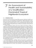
An example of ILA applied to terrestrial ecosystems is given in Figure 7.6. The self-entailment among
flows of different energy forms considered there refers to solar energy used for evapotranspiration, which
is linked to generation and consumption of chemical bonds in the biomass. That is, the four angles of
FIGURE 7.6 Terrestrial ecosystems.
© 2004 by CRC Press LLC
Impredicative Loop Analysis: Dealing with the Representation of Chicken-Egg Processes 189
Figure 7.6 refer to the forced congruence among two different forms of energy flowing in terrestrial
ecosystems: (1) solar energy to power evaporation of water associated with photosynthesis, which is
determining/determined by (2) biomass generated through photosynthesis, whose activity is used to
organize and control the evaporation of water.
Put another way, the chicken-egg loop stabilizing terrestrial ecosystems is described in Figure 7.6 as
an autocatalytic loop of two energy forms: (1) photosynthesis making biomass (storage of energy in the
form of chemical bonds), which makes it possible to use solar energy through evapotranspiration of
water and (2) solar energy invested in evapotranspiration of water, bringing nutrients to the leaves and
making possible the photosynthetic reactions required for making biomass. Also in this case, it is
possible to represent such a chicken-egg loop using a four-angle representation:
• Angle a—Due to the characteristic of the terrestrial ecosystem, a certain fraction of the
energy made available to the ecosystem through photosynthesis (extensive variable 1) is
used by the plants themselves. The fraction lost to autotrophic respiration—an overhead of
the plants—defines the NPP of an ecosystem, given a level of GPP (internal loss at the level
n-1).
• Angle β—The characteristics of the heterotrophic compartment of the terrestrial ecosystem

defines the distribution of the total biomass among different subcompartments (the shape of
the Eltonian pyramid, food web structure, or when adopting nonequivalent representations
of ecosystems—e.g., network analysis, different graphs). The combined effect of this
information will determine the ratio of SB /NPP (SB=standing biomass). This is still described
using fractions of extensive variable 1.
• Angle g—Due to the characteristic of the terrestrial ecosystem, there is a certain demand
of water to be used in evapotranspiration per unit of total standing biomass (total standing
biomass includes the biomass of heterotrophic and autotrophic organisms). This depends on
the turnover of different types of biomass (with known identities in different compartments)
and the availability of nutrients and way of transportation of them. This establishes a link
between investment of extensive variable 1 and returns of extensive variable 2 at the level n-
1 (over the autotrophic compartment).
• Angle d—This angle represents the ratio between two nonequivalent flows of energy
forms (two independent assessments) that can be used to establish a relation between:
1. The size of the dissipative system terrestrial ecosystem seen from the inside (extensive
variable 1), which is defined in size (total standing biomass and turnover time GPP/SB)
using a chain of identities (energy carriers×transformers×whole), chemical bonds
generated by photosynthesis making up flows of biomass across cornponents—total size
GPP. The internal currency expressed in GPP makes it possible to describe the profile of
investments of it inside the system over lower-level compartments (e.g., autotrophs and
heterotrophs).
2. The size of the dissipative systems as seen from the context (extensive variable 2). This is
the size of the energy gradient that is required from the context to stabilize the favorable
boundary conditions associated with the given level of GPP (incoming solar radiation
and thermal radiation into the outer space, which is supporting the process of water
evapotranspirations, plus availability of sufficient water supply).
Obviously, we cannot fully forecast what are the most important limiting factors or what are the
mechanisms more at risk in the future to stabilize such a power supply. But this is not a relevant issue
here. Given a known typology of terrestrial ecosystems, we can study the relation between the relative
flow of GPP and the solar energy for water transpiration associated with it, in terms of the relative

characteristics (extensive and intensive variables) of parts and the whole, represented as stabilizing an
impredicative loop of energy forms. The mapping of these two energy forms (extensive variables 1 and
2) can provide a reference value—a benchmark—against which to assess the size of the ecosystem (at
level n) and the size of its relative components (at level n-1) in relation to the representation of events
© 2004 by CRC Press LLC
Multi-Scale Integrated Analysis of Agroecosystems190
(intensive variables 3, associated with the identity of parts and lower-level elements) and the consumption
and generation of energy carriers/chemical bonds (at level n-2).
A detailed analysis of the self-entailment among characteristics of each one of the four angles (how
the identity of lower-level components affects the whole and vice versa) is the focus of theoretical
ecology applied to the issue of sustainability. Our claim is that ILA can provide a useful additional
approach to study such an issue. We propose the theoretical discussion provided in the Section 7.5 and
a few examples provided in Chapter 10 in Part 3 to support our claim. It is important to observe that
studying the forced relations between the characteristics of identities of elements (and the size of the
relative equivalence class) determining this impredicative loop in terrestrial ecosystems has to do with
how to define concepts like ecosystem integrity and ecosystem health, and how to develop indicators
of ecological stress. Even from this very simplified example, we can see that the concept of impredicative
loop can help to better frame these elusive concepts (integrity or health of natural ecosystems) in terms
of standard mechanisms of self-entailment among biological identities that are defining each other on
different levels and on different scales. Integrity and health can be associated with the ability of
maintaining harmony among the multiple identities expressed by ecological systems (the ability to
respect the forced congruence among flows exchanged across metabolic components organized in
nested hierarchies); see also last section of Chapter 6. Healthy ecosystems are those able to generate
meaningful essences for their components (more on this in Chapter 8).
As in the previous example of the 100 people on a desert island, the perceived identity of terrestrial
ecosystems is represented in Figure 7.6 in the form of an autocatalytic loop of energy forms that is related
to the simultaneous perception (and definition) of identities of lower-level components, higher-level
components and the congruence between functional relation and organized structures on the focal level.
Again, looking at energy forms is just one of the possible ways to look at this system (whenever we use x-
rays, we miss soft tissue). However, making explicit such a holarchic structure, in relation to a useful

selection of formal identities, can be valuable for studying the effect of perturbations. For example,
agriculture implies an alteration of the relations between key parameters determining the impredicative
loop described in Figure 7.6. Monocultures, by definition, translate into a very high NPP with little
standing biomass as averaged over the year, and a reduced fraction of heterotrophic respiration over the
total GPP. An analysis of the stability of ILA applied to agroecosystems can be used to look for indicators
of stress. A discussion of these points is given in Chapter 10 (e.g., Figure 10.13 through Figure 10.15). The
main point to be driven home from the ILA approach now is that whenever we deal with parameters that
are reciprocally entailed in a chicken-egg loop, we cannot imagine that it is possible to generate dramatic
changes in just one of them, without generating important consequences over the whole loop. That is,
whenever we decide to dramatically alter the holarchic structure of a terrestrial ecosystem, we have to
expect nonlinearity in the resulting side effects (the breaking of its integrity). The use of impredicative
loop analysis to study this problem should help in searching for mechanisms that can lead to catastrophic
events across different scales that can be useful for such a search (for more information, see Chapter 10).
7.2.5 Parallel Consideration of Several Impredicative Loop Analyses
An overview of the three impredicative loop analyses presented in Figure 7.2, Figure 7.5 and Figure
7.6 is given in Figure 7.7. Actually, these three formalizations of impredicative loops refer to three
possible ways of looking at energy forms relevant for the stability of agroecosystems. It is very important
to note that these three formalizations cannot be directly linked to each other, since they are constructed
using logically independent perceptions and characterizations of parts, the whole and contexts
(nonequivalent descriptive domains). The meta-model used for the semantic problem structuring is
the same, but it has been formalized (when putting numerical assessment in it) by referring to definitions
of energy forms, and useful energy that is specific for the set of identities adopted to represent the
autocatalytic loop. However, the three have some aspects in common, and this makes it possible to use
them in an integrated way when discussing, for example, scenario analysis.
These three applications of the same meta-model, useful for catching different aspects of a given
situation, required a tailoring of the general ILA on the specificity of a given situation. In this way it
© 2004 by CRC Press LLC
Impredicative Loop Analysis: Dealing with the Representation of Chicken-Egg Processes 191
becomes possible to build a set of integrated models reflecting different dimensions of analysis for a
specific problem. That is, scientists that want to use this approach to deal with a specific issue of sustainability

of an agroecosystem have to decide what are the relevant characteristics of the endosomatic autocatalytic
loop (which is associated with physiological, demographic and social variables) and exosomatic autocatalytic
loop (which is associated with both biophysical and socioeconomic variables), and critical factors affecting
the self-entailment of energy forms in a specific terrestrial ecosystem (which makes it possible to establish
a link with ecological analysis). The process through which scientists can decide how to make these
choices has been discussed in Chapter 5. According to what was said there, we should always expect that
different scientists asked to perform a process of multi-scale integrated analysis aimed at tailoring these
three meta-models in relation to a specific situation (e.g., by collecting specific data about a given society
perceived and represented at a given point in space and time as operating with a given terrestrial ecosystem)
will come up with different variables and models to represent and simulate different aspects. The same can
be expected with the direction of causality found in the analysis. Disciplinary bias (preanalytical ideological
choice implied by disciplinary knowledge) is always at work.
Put another way, the predicament described in Figure 7.4 (What are the independent and dependent
variables?), as well as all the other problems described in Chapter 3, can never be avoided, even when
we explicitly introduce in our analysis multiple identities defined on multiple scales. What can be done
when going for a multi-scale integrated analysis based on the parallel use of impredicative loop analysis
is to take advantage of mosaic effects. If the analyst is smart enough, she or he can try to select variables
that are shared by couples of ILAs. In this way, it becomes possible to look for bridges among
nonequivalent descriptive domains. As illustrated in Figure 5.9, it becomes possible to generate integrated
packages of quantitative models that are able to provide a coherent overview of different relevant
aspects of a given problem. In particular, they can be used to filter out incoherent scenarios generated
by simulations based on the ceteris paribus hypothesis. That is, they can be used to check the reliability
of predictions based on reductionist models.
7.3 Basic Concepts Related to Impredicative Loop Analysis and Applications
7.3.1 Linking the Representation of the Identities of Parts to the Whole and Vice Versa
The examples of four-angle figures presented in the previous section (e.g., Figure 7.7) are representations
of autocatalytic loops of energy forms obtained through an integrated use of a set of formal identities
defined on different hierarchical levels (Figure 7.1).
To explain the nature of the link bridging the representation given in Figure 7.1 and the representation
given in Figure 7.7, it is necessary to address key features associated with the analysis of the dynamic

FIGURE 7.7 The nested hierarchy of energy forms self-entailing each other’s identity.
© 2004 by CRC Press LLC
Multi-Scale Integrated Analysis of Agroecosystems192
energy budget of a dissipative system (Figure 7.8a). This alternative view provides yet another set of
attributes that can be used to represent autocatalytic loop of energy forms in hierarchically organized
dissipative systems. That is, the same network of elements represented in Figure 7.1 can be perceived
and represented in a nonequivalent way by dividing the components described at the level n-1 into
two classes (Figure 7.8.a): (1) those that do not interact directly with the environment (aggregated in
the compartment labeled “indirect”) and (2) those that do interact directly with the environment, e.g.,
by gathering input from the environment (aggregated in the compartment labeled “direct”). In this
view, the black box—seen as a whole (at level n)—can receive an adequate supply of required input
thanks to the existence of favorable conditions (at level n+1) and the work of the direct compartment
(at level n-1). This input feeding the whole can then be expressed in terms of an energy form, accounted
for by using an extensive variable (which we called extensive variable 1 in Chapter 6). This variable is
then used to assess how this total input is invested—within the black box—over its lower-level
compartments. This variable measures the size of the whole in relation to its parts. Therefore, we can
represent the total input, assessed using extensive variable 1, as dissipated within the black box in three
distinct flows (indicated by the three arrows in Figure 7.8.a):
1. A given overhead for the functioning of the whole
2. For the operation of the compartment labeled “indirect”
3. For the operation of the compartment labeled “direct”
The favorable conditions perceived at the level n+1, which make possible the stability of the
environmental input consumed by the whole system, in turn are stabilized because of the existence of
some favorable gradient generated elsewhere (level n+2), which are not accounted for in this analysis.
As noted, the very definition of environment is associated with the existence of a part of the descriptive
domain about which we do not provide causal explanations with our model. Favorable gradients,
however, must be available—to have the metabolism in the first place. These favorable gradients—
assumed as granted—are exploited thanks to the tasks performed by the components belonging to the
FIGURE 7.8
ILA: The rationale of the Meta Model.

© 2004 by CRC Press LLC
Impredicative Loop Analysis: Dealing with the Representation of Chicken-Egg Processes 193
direct compartment (the representation of energy transformations occurring at the level n-1). The
return by the energy input made available to the whole system (at level n) per unit of useful energy
invested by the direct compartment into the interaction with the environment (at level n-1) will
determine the strength of the autocatalytic loop of energy associated with the exploitation of a given
set of resources.
This integrated use of nonequivalent representations of relations among energy transformations
across levels is at the basis of the examples of impredicative loop analysis shown so far. The four-angle
figures are examples of coherent representation of relations among formal identities of energy forms,
which are generating an autocatalytic loop over five contiguous hierarchical levels (from level n-2 to
level n+2). The transformation associated with the upper level (environment) is assumed by default.
The general template for performing this congruence check is shown in Figure 7.8.b. The four-
angle figure combines intensive (angles) and extensive (segments) variables used to represent and
bridge the characterization of metabolic processes across levels. The figure establishes a relation between
a set of formal identities (given sets of variables) used to represent inputs to parts and the whole, and
their interaction with the environment across scales.
The two angles on the left side (α and β) refer to the profile of distribution of the total available
supply of energy carriers (or human activity or colonized land), indicated on the upper part of the
vertical axis, over the three flows of internal consumption, according to the mapping provided by
extensive variable 1. Angle α refers to the fraction of the total supply that is invested in overhead (e.g.,
for structural stability of lower-level components). Angle β refers to the profile of distribution of the
fraction of the total left after the reduction, which is implied by angle α, between direct and indirect
components. What is left of the original total—after the second reduction implied by angle β—for
operating the direct compartment, at this point, is the value indicated on the lower part of the vertical
axis. This represents the amount of extensive variable 1 (using still a mapping related to the internal
perception of size) that is invested in the direct interaction with the environment.
The two angles on the right (γ and δ) are used for a characterization of the interaction of the system
with the environment (the relation between the dark gray and black arrows in Figure 7.8a).
It is important to select a set of formal identities used to represent the autocatalytic loop (what

variables have to be used in such a representation in terms of extensive 1 and extensive 2) that is able
to fulfill the double task of making it possible to relate the perceptions and representations of relevant
characteristics of parts in relation to the whole (what is going on inside the black box) with characteristics
that are relevant for studying the stability of the environment (what is going on between the black box
and the environment). Obviously, both extensive variables 1 and 2 have to be observable qualities
(external referents have to be available to gather empirical information).
Therefore, the choice of identities to characterize an impredicative loop does not have as its goal
the establishment of a direct link between the dynamics inside the black box and the dynamics in the
environment. As has already been mentioned, this is simply not possible. The selection of two extensive
variables (1 and 2) that can be related to each other simply makes it possible to establish bridges among
nonequivalent representations of the identity or parts and wholes using variables that are relevant in
different descriptive domains and in different disciplinary forms of knowledge. The logically independent
ways of perceiving and presenting the reality, which are bridged in this way, must be relevant for a
discussion of sustainability.
For example, the three impredicative loop analyses presented in Figure 7.7 reflect three logically
independent ways of looking at an autocatalytic loop of energy forms according to the scheme presented
in Figure 7.8b. These three formalizations cannot be directly linked to each other in terms of a common
formal model, since they are constructed using logically independent perceptions and characterizations
of identities across scales. However, they:
1. Share a meta-model used for the semantic problem structuring. This meta-model can be
used to organize the discussion about how to tailor the selection of formal identities for
parts, the whole and environment (when putting numerical assessments in it) to specific
local situations.
© 2004 by CRC Press LLC
Multi-Scale Integrated Analysis of Agroecosystems194
2. Cover different aspects that are all relevant to a discussion of sustainability in relation to
different dimensions of analysis (physiological and sociodemographic first, techno-economic
second and ecological third).
3. Share some of the variables used for the characterization of the ILA.
7.3.2 An ILA Implies Handling in Parallel Data Referring to Nonequivalent

Descriptive Domains
Before getting into the description of key features and possible uses of ILAs (the typology of four-angle
figures introduced in the previous section), it is important to warn the reader about an important point.
The four-angle figures presented so far all share the same features: (1) graphic congruence in relation to
the extensive variables (rectangular shape of the four-angle figure) and (2) reasonable widths for all angles.
These two features are obtained because the data represented across the four quadrants are not to scale;
that is, the representation of angles and segments has been rescaled to keep the four-angle figure in a
regular shape. It should be noted that the choice of rescaling the representation of data over an ILA is
often an obliged one. In fact, if we want to compare the characteristics of parts to the characteristics of the
whole, by using the same combination of intensive and extensive variables, we should expect to find big
differences in the values found at different levels for (1) segments (in extensive terms, parts can be much
smaller than wholes—the brain compared with the body) and (2) angles (in qualitative aspects of different
specialized parts; a specialized part can have a value for an intensive variable that is much higher than the
average value found for the whole—the brain compared with the body). In this situation, if we decide to
keep the same scale of reference for the representation of both extensive (segments) and intensive (angles)
variables used to characterize parts and the whole, we should expect to obtain graphs that are very
difficult to read and use. An example of the difference between two four-angle figures based on a regular
scale and a rescaled representation is given in Figure 7.9.
The two four-angle figures in Figure 7.9 reflect the situation of the hypothetical farming system—size
of 100 ha (extensive variable 1 (EV1) referring to hectares of land)—described in the lower part of Figure
6.2. The two figures on the top represent a nonscaled graphical representation of the data set given in the
lower part of Figure 6.2. Two dynamic budgets are considered: (1) the dynamic budget of food (EV2)
(Figure 7.9a) and (2) the dynamic budget of money (EV2) (Figure 7.9b). The two figures on the bottom
present the same couple of ILAs but after rescaling the values taken by the variables across quadrants. With
this choice, the two reductions of the total available amount of extensive variable 1 divided among
internal components, which is associated with the two angles on the left (α and β angles in Figure 7.8b),
are reasonable: (1) a first overhead of 50% and (2) an allocation between direct and indirect of 10%. In this
situation, it is still possible to follow the numerical values on the graph, keeping the same scale across
quadrants. However, if we had used human activity as extensive variable 1 for studying the same two
dynamic budgets, we would have found that the two reductions referring to the two angles on the left (α

and β angles in Figure 7.8b) would have been (1) a first overhead of 90% and (2) an allocation between
direct and indirect around 50%. This would have made it impossible to handle a useful graphic representation
based on the representation of extensive variables using the same original scale.
A second qualitative difference that is relevant between the four figures shown in Figure 7.9 is between
the two figures on the left (Figure 7.9a and c), in which there is no congruence between (1) the requirement
of extensive variable 2 (food) consumed by the whole (at level n) and (2) the supply of extensive variable
2 produced by the compartment—land in production (at level n-1). On the contrary, the two figures on
the right, which are based on an extensive variable 2 of money (Figure 7.9b and d), are based on the
assumption that what is consumed by the whole system (at level n) is actually produced by the
compartment—land in production (at level n-1). A few quick comments about these differences are:
• Left side—The budget related to food is not in congruence (this farming system is producing
more food than it consumes). This can be used to classify this system in terms of a typology. For
example, this pattern can be associated with an agricultural system net producer of food. The
same ILA of land use (determination of a relation among identities of parts and the whole
© 2004 by CRC Press LLC
Impredicative Loop Analysis: Dealing with the Representation of Chicken-Egg Processes 195
defined across levels in relation to spatial flow of food) could have applied to a city. In this case,
the difference would have been very negative. This would have classified the system in the
typology “urban system, heavy food importer.” As discussed in the applications of Part 3, ILA
can be used to define typologies (in terms of both pattern of land use and human time use). In
the case of land use, this can help the characterization in quantitative terms of land use categories
that can be associated with socioeconomic variables. This could help to integrate economic
analysis to ecological analysis. Coming back to the example of ILA, given in Figure 7.9,
according to (1) existing demographic pressure (food eaten per hectare), (2) respect of ecological
processes (level of ecological overhead, which is very high in this example) and (3) available
technique of production (technical coefficients expressed at the level n-1), this farming system
can be characterized as having a low level of productivity of food surplus (400 kg of food
surplus produced per hectare of this typology of farming system). That is, from the perspective
of a crowded country needing to feed a large urban population, this would not be a typology
of farming system to sustain with ad hoc policies. Moreover, in this way, it is possible to individuate

key factors determining this characteristics: (1) the small difference between angle γ expressed
at the level n-1 (the yield of 2000 kg/ha obtained in the land in production) and angle δ
expressed at the level n (the level of consumption of the farming system, in terms of food
consumption per hectare) and (2) the huge ecological overhead (the difference between total
available land and managed available land). Obviously, we cannot ask too much of this very
simplified example. This figure is useful only to indicate the ability of this approach to establish
a relation among different dimensions of sustainability.
• Right side—The budget related to money flow is assumed to be in congruence. That is, the
flow of added value considered in the compartment land in production at the level n-1 (added
value related to the value of the subsistence crops plus added value related to the gross return of
the cash crop) has been used to estimate an average income for the farmers of this farming system
at the level n. This is just one of many possible choices. A different selection of economic indicators
(for example, using a combination of two indicators: net disposable cash for farmers and degree
of subsistence) would have provided a quite different characterization of this farming system. In
fact, only $15,000 in net disposable cash is generated in the simplified example considered in
Figure 6.2, whereas in terms of income, the account should be $25,000 when including also the
FIGURE 7.9 Different shapes of representations of ILA.
© 2004 by CRC Press LLC