Radio Propagation and Remote Sensing of the Environment - Chapter 4 potx
Bạn đang xem bản rút gọn của tài liệu. Xem và tải ngay bản đầy đủ của tài liệu tại đây (561.27 KB, 25 trang )
© 2005 by CRC Press
85
4
Geometrical Optics
Approximation
4.1 EQUATIONS OF GEOMETRICAL OPTICS
APPROXIMATION
In this chapter, we will discuss wave propagation problems in a medium with an
arbitrary law of permittivity coordinate dependence; that is, we will assume that the
permittivity has the form
ε
=
ε
(
r
) in the common case. The spatial variation slowness
of the permittivity is assumed to be similar to that for the Wentzel–Kramers–Brillouin
of permittivity at the wavelength scale. This property can be expressed as the
inequality:
(4.1)
As in the WKB method, we will utilize a solution to Maxwell’s equations in the
form of the asymptotic Debye series:
(4.2)
The value
ψ
is referred to as the
eikonal value
. We arrive at the system of connected
equations:
(4.3)
after substitution of the Debye series in Maxwell’s equations; members of the same
degree of
k
are equal to each other.
Zero-order equations are a system of homogeneous linear algebraic equations.
For the purpose of their nontrivial solution, it is necessary to reduce the determinant
to zero. This requirement leads to the equation for
ψ
(the eikonal equation). We can
obtain this equation fairly simply if
H
0
is expressed through
E
0
; also, we must take
into account the mutual orthogonality of vectors
E
0
,
H
0
, and
∇ψ
that follows from
∇ <<ln .ε k
E
Er
H
Hr
=
()
()
=
()
()
=
∞
=
∞
∑
e
ik
e
ik
ik
s
s
ik
s
s
ss
ψψ
,.
00
∑∑
∇ ×
+= ∇ ×
− =
∇ ×
+
ψε ψ
ψε
HE EH
HE
00 00
1
00,,
110 110
= −∇× ∇ ×
− = −∇×[], [],HEHEψ
TF1710_book.fm Page 85 Thursday, September 30, 2004 1:43 PM
(WKB) approximation carried out in Chapter 3. We assume again a small change
© 2005 by CRC Press
86
Radio Propagation and Remote Sensing of the Environment
the equations of the zero-order approximation. Now we can easily show that the
eikonal equation may be written down in the form:
(4.4)
The value:
(4.5)
represents the radiowave phase in the zero approximation, and eikonal
ψ
(in engi-
neering terminology) represents the electrical length passed by the wave. We assume
that the phases of components
E
0
and
H
0
do not depend on coordinates in the
approximation. Furthermore, in this approximation, these vectors are believed to be
real, including the initial wave phase at once in the wavelength. Certainly, small
additions to this phase may be made by calculation of the following items of
expansion.
In the zero-order approximation, the power flow density:
(4.6)
is directed along lines of the eikonal gradient. This fact allows us to refer to the zero
approximation as the
geometrical optics approximation
, which corresponds to the
small wavelength conversion (hence the term
optics
) and allows the wave propaga-
tion laws to be formulated in the language of geometry.
The validity of the geometrical optics approximation is defined by Equation
(4.1). If, as before, the scale of permittivity change is designated
Λ
, then the Debye
series is essentially expansion according to the inverse degree of large parameter
k
Λ
. Other conditions will be formulated later.
Let us assume, in the beginning, that the permittivity is a real value. We can
define the vector of wave propagation by the formula:
(4.7)
where
s
is the unitary vector, which is orthogonal to the equiphase surfaces. The
lines orthogonal to the surfaces of the eikonal constant value (to equiphase surfaces)
are called
rays
. Vector
s
is tangential to the rays and describes the wave energy
propagation direction.
If
τ
is the length along the ray, then the ray equation has the form
d
r
/
d
τ
=
s
.
Then,
∇ψ
=
s
d
/
ψ
/
d
τ
, and the eikonal equation becomes the common differential
equation:
(4.8)
∇
()
=ψε
2
.
ϕψ= k
SEH
000
=×
= ∇
cc
88
E
0
2
ππ
ψ
∇ =ψεs,
d
d
ψ
τ
ε=
TF1710_book.fm Page 86 Thursday, September 30, 2004 1:43 PM
© 2005 by CRC Press
Geometrical Optics Approximation
87
the solution of which is written in the form:
(4.9)
where
ψ
0
is the initial value of the eikonal
equation. Let us point out that use of the plus
sign was determined by extraction of the
square root in Equation (4.9). It is important
to note that we are dealing with a direct wave.
In the case of a backward wave, the minus sign
should be used. It is clear that the eikonal form
as a function of coordinates depends on the
ray along which the integration is provided.
We may use the orthogonal unitary vector
system of the normal
n
and the binormal
m
(Figure 4.1). Their changes along the
ray characterize its bending and torsion. The Frenet–Serre formulae:
(4.10)
are known from differential geometry.
29
The value
ρ
is the ray curvature radius, and
χ
is its torsion. The vectors
s
,
n
, and
m
are the basis of the curved-line coordinate
system formed by the ray ensemble and equiphase surfaces. This system is often
referred to as the
ray coordinates
. Equation (4.9) is the eikonal equation solution in
the ray coordinates system.
Let us use the eikonal equation in Equation (4.8) to calculate
ρ
and
χ
. We must
take the gradient of both parts to obtain:
.
Thus, it follows that:
(4.11)
Equation (4.11), together with the first Frenet–Serre equation, allows us to determine
the radius of ray curvature:
(4.12)
ψτ ψ ετ τ
τ
()
=+
′
()
′
∫
0
0
d ,
FIGURE 4.1 The orthogonal uni-
tary vector system.
n
m
s
d
d
d
d
d
d
sn n s
m
m
n
τρ τ ρ
χ
τ
χ==−− =,,
d
d
s ε
τ
ε
()
= ∇
d
d
s
ss
τ
εε= ∇−⋅∇
()
ln ln .
1
2
22
ρ
εε= ∇
()
−⋅∇
()
ln ln .s
TF1710_book.fm Page 87 Thursday, September 30, 2004 1:43 PM
© 2005 by CRC Press
88
Radio Propagation and Remote Sensing of the Environment
If angle
α
between the direction of the ray and the direction of the permittivity is
introduced, then:
(4.13)
Further, it is simple to establish that:
(4.14)
We must now derive equations for fields
E
0
and
H
0
. First of all, let us point out that
the wave is transversal in zero-order approximation, so its components may be
represented in the form:
(4.15)
On the basis of Equation (4.15) and after some not very complicated calculations,
25
we can define the conditions that connect the electrical field components directed
along the normal and along the binormal:
(4.16)
Returning to the local cylindrical coordinate system:
, (4.17)
we can easily obtain from Equation (4.16) the transfer equation:
(4.18)
1
ρ
εα= ∇ln sin .
nss ss
m
= ∇−⋅∇
()
= ⋅∇
()
=
ρε ερ εln ln ln ,
[[] ln ,
.
sn s
n
m
ns m
⋅ = ⋅∇
= ⋅ = ⋅⋅∇
()
ρε
χ
τ
d
d
EnmH sE nm
000
=+ = ×
= −
()
EE EE
nm nm
,.εε
220
2
εεεχε
ε
∇ + ∇
⋅
()
+ ∇⋅ +=
∇ +
EE E E
EE
nn n m
m
() ,ss
mmmn
∇
⋅
()
+ ∇⋅ − =() .εε χεssEE20
EE
n
==EE
0m0
cos , sinϑϑ
∇⋅
()
= ∇⋅ =εE
0
2
sS0
TF1710_book.fm Page 88 Thursday, September 30, 2004 1:43 PM
© 2005 by CRC Press
Geometrical Optics Approximation
89
and the equation of torsion:
(4.19)
Equation (4.18) conveys the energy conservation law. The solution to Equation (4.19)
may be written as:
(4.20)
which describes the law of wave polarization elliptical rotation without changing its
form (Rytov’s law).
We may rewrite Equation (4.18) in another form by using Equation (4.7). Then,
in the ray coordinates,
,
and the solution is obvious:
(4.21)
This expression can be written down in another form by using the ray divergence.
Let us insert the ray coordinates
ξ
,
η
, and
τ
. Coordinate
τ
is directed along the rays,
while the other two coordinates are orthogonal to it and are directed, for example,
along the vectors of normal and binormal. The Jacobian of the transition from
Cartesian coordinates (x,y,z) to ray coordinates is given by the formula:
(4.22)
The ray tube is defined as a ray family passing through the area
d
ξ
d
η
near a point
with coordinates (
ξ
,
η
,
τ
). The square of the surface element perpendicular to the
s ⋅∇
()
− =ϑχ0.
ϑϑ χτ τ
τ
=+
′
()
′
∫
0
0
d ,
d
d
E
E
0
0
τ
ψ
ε
+
∇
=
2
2
0
EE
00
τ
ψτ
ετ
τ
τ
()
=
()
−
∇
′
()
′
()
′
∫
0
1
2
2
0
exp d
D ξητ
∂
∂ξ
∂
∂η
∂
∂τ
∂
∂ξ
∂
∂η
∂
∂τ
∂
∂ξ
∂
∂η
∂
,,
()
=
xxx
yyy
zzz
∂∂τ
.
TF1710_book.fm Page 89 Thursday, September 30, 2004 1:43 PM
© 2005 by CRC Press
90
Radio Propagation and Remote Sensing of the Environment
direction of the rays (equiphase surface) equals
Dd
ξ
d
η
. The volume of the ray tube
element equals
Dd
ξ
d
η
d
τ
. Applying vector analysis to Equation (4.8), it is a simple
matter to obtain:
(4.23)
We will use this formula for the volume bounded by the ray coordinates and will
reduce the volume to zero; moreover, we take into account that (
n
·
s
) = 0 at the
sides of the tube. We then have:
or
(4.24)
Instead of Equation (4.21), we obtain:
. (4.25)
This result is transparent from the physical point of view: Due to the law of energy
conservation, the field amplitude changes together with changes in the cross section
of the ray tube. The second condition of the geometrical optics approximation
validity follows from Equation (4.25). It is not valid where
D
(
τ
) = 0. Areas where
the Jacobian is reduced to zero are called
caustics
and round out the ray family. In
WKB approximation, corresponds to the caustics plane. For more details about
caustics, refer to Kravtsow and Orlov.
27
Up to this point, it was assumed that permittivity is the real value. Let us now
turn to the more realistic case of weak absorption in the media and, related to this,
complex permittivity. We can still use Equation (4.4), but the eikonal itself must
now be complex (i.e.,
ψ
=
ψ′
+
i
ψ′′
). It is apparent that the eikonal imaginary part
describes wave attenuation due to absorption and, being multiplied by the wave
number, is equal to the coefficient of extinction. The separation of real and imaginary
parts in Equation (4.4) leads to a pair of equations concerning
∇ψ′
and
∇ψ′′
. It is
difficult to find the solution of these equations, particularly because it is necessary
to know the angle between
∇ψ′
and
∇ψ′′
.
∇ = ∇⋅ ∇ = ⋅∇
()
= ⋅
()
∫∫
23 3 2 2
ψψ ψεddd d
SS
rrnrnsr() .
VVV
∫∫
∇
()
=+
()
+ −
()
2
ψτξητ τ τεττ τετξηDddd D d d D dd[()()]
∇
=
() ()
2
ψ
ε
τ
ετ τ
d
d
Dln .
EE
00
τ
ε
ετ τ
()
=
() ()
() ()
()
00
0
D
D
TF1710_book.fm Page 90 Thursday, September 30, 2004 1:43 PM
particular, the turning point, which we mentioned in Chapter 3 with regard to the
© 2005 by CRC Press
Geometrical Optics Approximation
91
We will now consider a simple but common case of small absorption in the
sense that
ε′′
<<
ε′
and (
∇ψ′′
) << (
∇ψ′
)
2
. The pair of equations then acquires the
form:
(4.26)
The first equation is solved as before and the second one is transformed to the form:
.
Hence, it follows that:
(4.27)
We will now briefly address the case of anisotropic media, including the iono-
sphere. In this case, the eikonal equation is broken down into two equations — one
for ordinary and one for extraordinary waves:
28
(4.28)
These waves, generally speaking, can be considered to be independent if the length
of the beating between them is much smaller than the scale of the medium inhomo-
geneities. The beating length is estimated by the value:
(4.29)
The substitution of specific values (
f
= 10
8
Hz,
N
= 2 · 10
6
cm
3
, H
0
= 0.5 Oersted)
gives the estimation
l
≈
10 km. It would seem that the independence of ordinary
and nonordinary waves can be broken with increasing frequency and, correspond-
ingly, with increasing beating length. This is not so, however, because in this case
the wave relation coefficient decreases with increases in frequency;
28
therefore,
ordinary and extraordinary waves are practically always independent for the ultra-
high-frequency and microwave bands for the ionosphere of Earth.
The ray trajectories of ordinary and extraordinary waves practically coincide,
because their refractive indexes differ little in the range of waves being considered
here, which allows us to develop a formula to calculate the polarization angle rotation
value due to the Faraday effect:
∇
′
()
=
′
∇
′
∇
′′
()
=
′′
ψε ψψε
2
2,.
d
d
′′
=
′′
′
ψ
τ
ε
ε2
′′
()
=
′′ ′
()
′′
()
′
∫
ψτ
ετ
ετ
τ
τ
1
2
0
d .
∇
()
= ∇
()
=ψψ
oo
2
2
2
2
nn
ee
,.
l
c
nn
cf
ff
f
NH
e
=
−
()
≅ =
⋅
−
21310
2
2
42
0
π
ωβ
opH
cos
.
.
TF1710_book.fm Page 91 Thursday, September 30, 2004 1:43 PM
© 2005 by CRC Press
92
Radio Propagation and Remote Sensing of the Environment
(4.30)
Finally, we will calculate the Doppler frequency shift for wave propagation in an
inhomogeneous medium. For this purpose, let us refer back to Equation (2.97) and
rewrite it as follows:
(4.31)
It is easy to see that the Doppler shift value is proportional to the velocity component
directed along the ray (ray velocity).
4.2 RADIOWAVE PROPAGATION IN THE
ATMOSPHERE OF EARTH
The atmosphere of Earth can be considered, in the first approximation, as a spher-
ically layered medium where the permittivity is a function of the radius beginning
at the center of the Earth. We do not include in our consideration here the changes
in atmospheric parameters along the surface of the Earth that take place at the
transition from day to night (light to shadow), along frontal zones with significant
changes of air temperature, and so on. It should be supposed that
ε
=
ε
(
R
),
∇ε
=
R
/
R
(
d
ε
/
dR
), etc. It is believed, that, on average, 1/m in the
troposphere near the surface of Earth; therefore, the geometrical optics approxima-
tion is highly accurate for the given wave range. The vertical gradient in the iono-
sphere is even smaller, so applying the geometrical optics approximation is still
appropriate. Although the permittivity of air does differ from unity, the difference
is insignificant and we can assume it to be equal to unity without causing problems.
We can prove rather easily the permanency of vector along the ray
trajectory; hence, we can make the statement that in the case of a spherically layered
medium the ray trajectories are plane curves. The product:
(4.32)
is invariant along the ray, where the constant
η
is determined from the initial
conditions. If, for example, a ray left Earth at angle
α
0
, then , where
the radius of the Earth
a
≅
3
established on the ray prolongation until the surface of the Earth. Equation (4.32)
is often referred to as Snell’s law for spherically layered media.
We will now consider the situation when a ray passes by the surface of Earth
ε
→
1, and
R
sin
α
→
p
, where
p
is the
aimed distance
(a term borrowed from the theory of particle scattering). In
this case, a ray turning point occurs at R = R
m
, where α(R
m
) = π/2.
Ψ
Fo
2
= −
()
′
≅
′
()
′
()
′
ω
τ
π
ττβ
2
2
3
22
0
c
nnd
e
mc f
NH
e
cos τττ
ττ
()
′
∫∫
d .
00
ωψε
d
kk= −⋅∇
()
= −⋅
()
vsv.
gddR
ε
ε= ≅− ⋅
−
810
8
ε[]Rs×
εαηRR R
() ()
=sin ,
ηε α=
00
a sin
TF1710_book.fm Page 92 Thursday, September 30, 2004 1:43 PM
6.4 · 10 km (see Figure 4.2). The starting point may be
(Figure 4.3). Far from the atmosphere of Earth, (R)
© 2005 by CRC Press
Geometrical Optics Approximation 93
It is convenient, in our case, to write the eikonal equation for the spherical
coordinate system with the center coinciding with the center of the Earth. This
system can be chosen in such a way as to take into account the plane character of
the ray trajectories so that the eikonal will not depend on the azimuthal angle ϕ.
The eikonal equation can be written as:
(4.33)
in our chosen system of coordinates. Proceeding according to the variable separation
method, we will seek a solution as the sum:
(4.34)
Combining Equations (4.33) and (4.34) and taking into account the initial conditions,
we obtain:
(4.35)
where R
0
and θ
0
are the coordinates of the initial ray point. The sign before the
integral is chosen depending on the type of ray branch: the plus sign for the ascendant
branch and the minus sign for the descendent branch. For geometrical reasons,
(4.36)
FIGURE 4.2 Radio propagation from the
surface of the Earth.
FIGURE 4.3 Propagation radio wave along
the surface of the Earth.
a
α
ξ
R
P
R
m
ξ
∂ψ
∂
∂ψ
∂θ
ε
R
R
R
+
=
()
2
2
2
1
ψθψ ψθ
θ
RR
R
,.
()
=
()
+
()
ψθηθθ ε
η
RR
R
dR
R
R
,,
()
= −
()
±
′
()
−
′
′
∫
0
2
2
0
Rd
dR
R
R
θ
α
η
ε
η
==
± −
tan
2
2
TF1710_book.fm Page 93 Thursday, September 30, 2004 1:43 PM
© 2005 by CRC Press
94 Radio Propagation and Remote Sensing of the Environment
and
(4.37)
The rule for choosing the appropriate sign is the same as for the previous case. As
a result, we now have:
(4.38)
It follows from Equation (4.38) that:
Taking into account Equation (4.21), the equality can be derived as:
(4.39)
As before, the result obtained corresponds to the WKB approximation.
m
with the caustic surface and additional caustic phase shift occurs.
12,19
Without going
into detail regarding the calculation, we should point out that, in this case,
(4.40)
and cos α approaches zero close to the turning point; the amplitude, formally
calculated in the geometrical optics approximation, tends to infinity, which empha-
sizes once again that the geometrical optics approximation is inapplicable in areas
close to caustics.
θθ η
ε
η
− =±
′
′
−
′
∫
0
2
2
2
0
dR
R
R
R
R
.
ψθ
ε
εη
R
RRdR
RR
R
R
,.
()
=±
′′
()
′
′
()
′
−
∫
22
0
∇ =
−
−
2
2
2
2
2
1
2
ψ
ε
η
ε
η
d
dR
R
R
.
EE
00
R
RR
RR
()
=
()
−
()
−
()
=
εη
εη
ε
0
2
0
2
22
1
4
0
000
0
cos
cos
.
α
εαR
()
()
E
0
ψθ
ε
ε
ε
ε
R
RRdR
RR p
RRdR
R
,
()
=
′′
()
′
′
()
′
−
+
′′
()
′
′
(
22
))
′
−
−
∫∫
Rp
R
R
R
R
mm
22
2
0
π
,
TF1710_book.fm Page 94 Thursday, September 30, 2004 1:43 PM
When the ray passes through point R = R (Figure 4.3) it comes into contact
© 2005 by CRC Press
Geometrical Optics Approximation 95
The important ray parameter is the
angle of refraction characterizing the
degree of its bending. The differential of
this angle is defined as the angle between
the ray direction in infinity nearby points
τ
and τ + dτ (Figure 4.4). The differential
value (let us represent it as ξ) is determined
from the equality =
–msin(dξ). Let us now use the expansion:
,
Equation (4.11), and the relation allow us to obtain:
(4.41)
Hence, it follows that:
and
(4.42)
This expression will have the form:
(4.43)
0
corresponding points of the ray trajectory are practically outside the atmosphere.
The upper limit in the last integral can be set at infinity, and we can write:
FIGURE 4.4 Refraction angle differen-
tials and changing optical density.
s (τ + dτ)
s (τ)
d ξ
[() ( )]ssτττ×+d
ss
s
ττ τ
τ
τ+
()
=
()
+d
d
d
d
sR m×
=Rsinα
d
d
d
dR
R
ξ
τε
ε
α= −
()
1
2
sin .
ξ
ε
ε
ατ
ε
ε
α
τ
= −
′
′
= −
′
′
∫
1
2
11
2
1
00
d
dR
d
d
dR
dR
R
R
sin tan
ττ
∫
ξη
η
ε
ε
εη
R
R
dR
dR
dR
RR
R
R
,
()
= −
′
()
′
()
′
′
′
()
′
−
∫
2
1
22
0
ξ
ε
ε
ε
ε
ε
ε
= −
′
′
′
−
−
′
′
′
∫
p
d
dR
dR
Rp
p
d
dR
dR
R
R
R
m
2
1
2
1
22
0
222
−
∫
p
R
R
m
.
TF1710_book.fm Page 95 Thursday, September 30, 2004 1:43 PM
for the rays shown in Figure 4.3. In particular, if R and R are sufficiently large, the
© 2005 by CRC Press
96 Radio Propagation and Remote Sensing of the Environment
(4.44)
Angle ξ, in this critical case, is the angle of wave scattering in the spherically layered
atmosphere.
When the reception of waves radiated by highly disposed sources (for example,
artificial satellites) is realized on the surface of the Earth, angle ξ is equal to an error
in determination of the angle position of these sources. This error in determination
of the zenith angle can be written as:
(4.45)
By determining this error from data measured at different values of angle α
0
, we
can define the altitude profile of the atmospheric permittivity using the inverse
problems technique.
Let us point out that Equation (4.45) can be rewritten as:
(4.46)
Let us now extend the radius of the Earth to infinity, thereby transforming the
problem to one involving a plane-layered atmosphere. As a result we have:
(4.47)
The last integral is calculated at any function ε(ς). For our purposes here, we can
substitute Then,
(4.48)
So, the value of the refraction angle for a plane-layered medium depends only on
the permittivity values at the terminal points of the ray trajectory (Laplace theorem).
ξ
ε
ε
ε
pp
d
dR
dR
Rp
R
m
()
= −
−
∞
∫
1
22
.
ξα
εα
ε
ε
εε α
0
00
2
0
22
0
2
1
()
= −
−
∞
∫
a
d
dR
dR
Ra
a
sin
sin
.
ξα
εα
ες
ες
ς
ες ς ε
0
00
2
0
2
2
1
()
= −
()
()
()
+
()
−
a
d
d
aa
sin
ssin
.
2
0
0
α
ςd
∞
∫
ξα ε α
ες
ες
ς
ες ε α
ς
000
0
2
0
0
1
()
= −
()
()
()
−
sin
sin
.
d
d
d
∞∞
∫
sin ( ) ( ) sin .ας ε ες α=
00
ξα ε α α
0000
()
=
()
−arcsin sin .
TF1710_book.fm Page 96 Thursday, September 30, 2004 1:43 PM
© 2005 by CRC Press
Geometrical Optics Approximation 97
Let us point out that this result is easily obtained using Snell’s law for plane-layered
media. The small deviation of the permittivity from unity allows the use of the Taylor
expansion to obtain:
(4.49)
As previously mentioned, the Doppler frequency shift must be considered in the
case of moving sources:
(4.50)
according to Equation (4.31). Here, v
R
= dR/dt is the radial velocity and Ω
θ
= dθ/dt
is the angular velocity. The Doppler frequency shift depends not only on movement
parameters but also on the atmospheric characteristics, because angle α is determined
by the refraction phenomenon.
4.3 NUMERICAL ESTIMATIONS OF ATMOSPHERIC
EFFECTS
Let us now turn to numerical estimation of atmospheric effects that occur during
radio propagation of ultra-high-frequency and microwave bands. Let us begin with
the troposphere. The altitude dependence of atmospheric air permittivity can be
generally described by:
31
(4.51)
Here, as before, ς is the altitude above land, ε
0
– 1 ≅ 6 · 10
–4
defines the near-land
value of the air permittivity, and H
T
≅ 8 km is the frequently used troposphere height.
The parameters of this exponential model of the troposphere depend on meteoro-
logical conditions and, particularly, on geographical location. So, the parameters
used here should be considered only as reference ones that are close to average,
although the real values are not very different from these values. Estimations show
that the integral of refraction for this model can be represented in the form:
32
(4.52)
ξα
ε
α
0
0
0
1
2
()
=
−
tan .
ωεα α
θdR
= − +
kv RR Rcos ( ) sin ( )Ω
ες ε
ς
()
=+ −
()
−
11
0
exp .
H
T
ξα
ε
α
0
0
00
1
2
()
=
−
()
tan ,Zs
TF1710_book.fm Page 97 Thursday, September 30, 2004 1:43 PM
© 2005 by CRC Press
98 Radio Propagation and Remote Sensing of the Environment
where
(4.53)
and a
e
8500 km is the so-called equivalent radius of the Earth. At s
0
>> 1, Z(s
0
) ≅ 1,
and
(4.54)
which corresponds to the plane-layered troposphere approximation. At s
0
<< 1, which
corresponds to the angles being close to π/2, and the refraction angle
is defined as follows:
(4.55)
It follows from Equation (4.55) that the maximum value of the refraction angle is
ξ ≅ 1.2 · 10
–2
.
Let us now consider the influence of the troposphere effect on distance mea-
surement — for example, for spacecraft using radio equipment. The time of the
signal traveling from the object to the reception point is directly measured in this
case. This time is easily converted to the electrical length of the propagation track
(eikonal). The eikonal value depends on the properties of the troposphere, so we
will now address formal calculation of the distance using a known eikonal value, as
well as the error involved. This error value is equal to the difference ,
where is the eikonal value in the absence of the atmosphere. This difference is
approximately equal to:
32
(4.56)
If s
0
>> 1,
(4.57)
Zs se e ds s
a
H
s
s
e
s
00 0 0
2
2
0
2
2
0
()
==
−
∞
∫
,cos,
T
α
ξα
ε
α
0
0
0
1
2
()
≅
−
tan ,
Zs s
00
()
≅π
ξ
επ
≅
−
0
1
22
a
H
e
T
.
∆ψ ψ ψ= −
′
0
′
ψ
0
∆ψ
ε
α
=
−
()
()
0
0
0
1
2
H
Zs
T
cos
.
∆ψ
ε
α
≅
−
()
0
0
1
2
H
T
cos
,
TF1710_book.fm Page 98 Thursday, September 30, 2004 1:43 PM
© 2005 by CRC Press
Geometrical Optics Approximation 99
which corresponds to the plane-layered atmosphere approximation. When s
0
<< 1,
(4.58)
The maximum value is ∆ψ ≅ 10
2
m for the parameters used here.
Now, we turn our attention to calculation of the frequency Doppler shift. In
doing so, we will be interested in that part of the frequency change that is determined
using a case typical for planet occultation observations;
32
the method presented here
has been used for measurement of troposphere parameters.
35
Let the transmitter be
at point T, the receiver at infinity, and the ray come to the receiver at sighting distance
p. Angle α in Equation (4.50) is measured, in this case, at point . At this point,
, and if radius R
T
is large enough; ξ = 0 in the absence of
atmosphere; and the corresponding frequency shift is:
(4.59)
where
(4.60)
is the platform velocity along the undisturbed (by atmosphere) ray (sighting line).
Having done the expansion for small-angle ξ, we now have:
(4.61)
Here,
(4.62)
is the velocity component perpendicular to the sighting line. To estimate the effect,
let us assume that ξ = 2.4 · 10
–2
and v
⊥
= 8 km/sec (for an artificial satellite of Earth).
Thus, ∆ω
T
/ω ≅ 6.4 · 10
–7
.
When the radiation reception occurs on Earth, we must refer to Equation (4.50),
which we can rewrite to take into account the trajectory equation, Equation (4.32):
∆ψ
επ
≅
−
0
1
22
aH
eT
.
R
T
αθξR
T
()
= −
ε R
T
()
= 1
ˆ
,ω
ω
d
v
= −
=
c
vv R
=
=+
RT
cos sinθθ
θ
Ω
∆ω
ω
ωω
ω
ξ
T
c
=
−
= −
⊥dd
v
ˆ
.
vv R
⊥
= −
RT
sin cosθθ
θ
Ω
TF1710_book.fm Page 99 Thursday, September 30, 2004 1:43 PM
by the troposphere properties. Let us first discuss the bypass variant (Figure 4.3)
© 2005 by CRC Press
100 Radio Propagation and Remote Sensing of the Environment
Expansion when parameters ε
0
– 1 and ξ are small leads to the formula:
(4.63)
We have supposed so high altitude of the radiation source that we can assume
If now we use formula (4.52) for medium refraction the result will be
(4.64)
For the common example of an artificial satellite on a circular orbit around Earth,
the radial velocity may be expected to be equal to zero. Further, we can assume that
aΩ
θ
= 8 km/sec, a
0
= π/2, and ∆ω
T
/ω ≅ 8 · 10
–9
at these parameters.
For the analysis of ionospheric effects, we will work primarily with spacecraft
orbits that are above the ionospheric electron concentration maximum. Again, let us
first estimate the refraction angle value. In this case, knowledge of the angle between
the ray direction at the point of reception on Earth and the sight line to the radiation
source is more important than knowledge of the refraction angle itself. Let us indicate
this angle as δ. We can show that, approximately,
32
(4.65)
where R is the spacecraft altitude (distance from the center of Earth), R
m
is the
altitude of the electron concentration maximum, , and the
function:
(4.66)
is the electron content at the altitude of the radiation source. Let us suppose for
numerous estimations that R >> a, R
m
= a + z
m
, and z
m
= 300 km. We can propose
the average estimation of for the total electron content. Then,
ωεεαεα
θd
R
k
v
R
RR a a= −−+
() sin sin .
2
0
22
00 0
Ω
∆ω
ω
ε
αξα
α
TR
c
= −
−
−
−
ava
RR
0
00
0
2
1
2
sin cos
sin
aa
22
0
sin
.
α
θ
+
Ω
ε
()
.R = 1
∆ω
ω
εα
α
TR
c
= −
−
()
−
()
−
00
0
0
2
1
2
1
a
Zs
va
RR
sin
sin
aa
22
0
sin
.
α
θ
+
Ω
δ
π
α
α
=
()
−
e
f
aR A R N R
AR AR a
2
2
0
3
0
2m
mt
m
sin ( ) ( )
() cos
,
AR R a() sin= −
222
0
α
NR NRdR
a
R
t
() ( )=
′′
∫
N
t
cm()∞≅ ⋅
−
310
13 2
TF1710_book.fm Page 100 Thursday, September 30, 2004 1:43 PM
© 2005 by CRC Press
Geometrical Optics Approximation 101
(4.67)
From here, for instance, δ = 8.4 · 10
–4
(3′) for f = 108 Hz and α
0
= 60°.
Let now estimate the dependence of the eikonal value (electrical length) on the
ionosphere. Here, for the same reasons:
. (4.68)
where ∆ψ has a negative value in the ionosphere due to the fact that the radiowave
phase velocity in plasma is greater then the speed of light. The maximum effect
takes place at the distance from Earth where the ray penetrates through the entire
ionosphere thickness. In this case, we must substitute the total electron content value
in Equation (4.68) to obtain:
(4.69)
For α
0
= 60° and f = 10
8
Hz, ∆ψ = –2.15 · 10
3
m. Note that the effect would be
positive and ∆L
g
= –∆ψ if we dealt not with the phase correction for the distance
(i.e., for the eikonal) but with the so-called group correction ∆L
g
(i.e., refractive
correction on the distance defined by the signal group velocity).
The Doppler effect can be written as:
(4.70)
The main dependence here, again, is connected with the electron content. Having
already became standard, our estimations give, with α
0
= 60° and f = 10
8
Hz, a value
of the order of for the relative frequency change.
Finally, we now consider the Faraday rotation of the polarization plane. Accord-
ing to Equation (4.30),
(4.71)
The magnetic field of Earth coincides with the field of the magnetic dipole, having
magnetic moment M (M ≅ 8.1 · 10
25
CGSE);
33
therefore,
δ
α
α
I
f
=
⋅
−
()
173 10
1091
12
0
22
0
32
.sin
.sin
.
∆ψ
π
= −
()
e
f
RN R
AR
t
2
2
2m
m
m
()
∆ψ
α
= −
⋅
−
121 10
1091
21
22
0
.
.sin
.
f
∆
Ω
ω
ω
δα α
α
θ
I
R
c
=
−
+
aa
RR a
v
cos sin
sin
00
222
0
.
10
8−
Ψ
F
2
m
=
′
()
⋅
()
∫
e
cf
Nd
3
22
0
0
2π
τ
τ
Hs.
TF1710_book.fm Page 101 Thursday, September 30, 2004 1:43 PM
© 2005 by CRC Press
102 Radio Propagation and Remote Sensing of the Environment
(4.72)
where µ is the angle between M and R. At these conditions,
. (4.73)
With these assumptions, we obtain the following approximate calculation:
(4.74)
Here Kolosov et al.
31
provides an
example of the calculation of ∂/∂τ′(cos µ/R′
2
). Here, we provide an estimation, having
assumed on average that:
where µ
0
is the magnetic latitude of the ground point, and we obtain:
, (4.75)
assuming that 〈sinµ
0
〉 = 0.5 and substituting the previous values of the parameters
for high-altitude sources (e.g., artificial satellites). We obtain Ψ
F
≅ 38 radians for
the traditional α
0
= 60° and f = 10
8
Hz.
4.4 FLUCTUATION PROCESSES ON RADIOWAVE
PROPAGATION IN A TURBULENT ATMOSPHERE
The atmosphere model adopted in the previous sections is assumed to be homoge-
neous on a large scale with a regional character and parameters dependent on climate
conditions in general. These parameters (for example, temperature) change slowly
throughout the day and vary according to season, so they have both diurnal and
seasonal trends. Because it is large scale, this model allows us to use the spherically
layered atmosphere approximation and gives us the opportunity, as we have shown,
to describe radiowave propagation processes in general. The described effects change
H
MR M
0
32
≅−∇
= −∇
RR
cos
,
µ
Ψ
F
2
M
2m
= −
′
()
′
′
∫
e
cf
N
R
d
3
22 2
0
π
τ
∂
∂τ
µ
τ
τ
cos
Ψ
F
2
M
2m
= −
′
′
−
′
′
e
cf
R
Ra
R
3
22
222
0
2
π
α
∂
∂τ
µ
sin
cos
()
′
=RR
NR
t
.
RR RR RR RR=>=<
mm m
when and when .
∂
∂τ
µµ
′
′
≅−
′
cos sin
,
RR
2
0
3
2
Ψ
F
=
⋅
−
212 10
1091
17
22
0
.
.sinf α
TF1710_book.fm Page 102 Thursday, September 30, 2004 1:43 PM
© 2005 by CRC Press
Geometrical Optics Approximation 103
only slowly, with typical periods of at least 1 hour; however, along with these rather
slow processes much faster ones also occur with periods on the order of seconds.
They have a random character and are generated by turbulent pulsation in the
atmosphere. As experience shows, these turbulent pulsations initiate small fluctua-
tions of medium permittivity. Because of the accumulation phenomenon, fluctuations
in the radiowave parameters (amplitude, phase, frequency) may not be small, and
we must study these fluctuations, because, in some cases, they generate noticeable
effects with regard to radiowave propagation in the troposphere and ionosphere of
Earth.
We will now provide a brief description of the statistical properties of turbulent
pulsation in the atmosphere. We must first consider permittivity as a stochastic
function of coordinates and time. The last dependence is neglected in the first
approximation; due to the great velocity of radiowave propagation, the signal man-
ages to pass from the transmitter to the receiver in a time that is much less than
typical periods of turbulent fluctuations. This allows the medium to be considered
as unchangeable and we may take into account only spatial changes in the permit-
tivity; hence, the approximation should be assumed to be a random function of
coordinates.
Let us assume that the medium is statistically homogeneous and suppose for
simplicity that 〈ε(r)〉 = 1. Then,
(4.76)
where µ(r) is a random coordinate function with a zero average. Further, it is
supposed that the intensity of the permittivity fluctuations is small; that is, 〈µ
2
〉 <<
1. This gives us the opportunity to consider µ to be a small value on the whole,
based on the small probability of its having large values; therefore, the probability
of significant local fluctuations of the radiowave parameters is also small. We also
need the spatial correlation function of the permittivity:
(4.77)
The introduced function depends only on the differential vector r = r
2
– r
1
due to
the statistic homogeneity of the turbulence field. In addition, we will assume statis-
tical isotropy of the turbulence. On this basis, the correlation function depends only
on the distance between the points of correlation and does not depend on the direction
of vector r connecting these points. Let us introduce the spatial spectrum of turbu-
lence:
(4.78)
ε µ() (),rr=+1
K
ε
µµrr r r
12 1 2
,.
()
=
()()
KK
ε
π
qrr
qr
()
=
−⋅
∫
1
8
3
3
()ed
i
.
TF1710_book.fm Page 103 Thursday, September 30, 2004 1:43 PM
© 2005 by CRC Press
104 Radio Propagation and Remote Sensing of the Environment
The correlation function is expressed through its spatial spectrum by the relation
(4.79)
The function represents the spectral density of the power of the permittivity
fluctuations inside the wave vector interval (q, q+dq). We can easily show that the
isotropy of the correlation function leads to isotropy of the spectral density.
We will often use the following formula for the spectrum:
(4.80)
Here, by convention, the wave number q
0
corresponds to the maximum (outer)
turbulence scale and q
m
is the minimum (inner) scale. Let us call value ν the spectral
index (although this term is often given to the double value 2ν). It is often assumed
that ν = 11/6 for the case of tropospheric turbulence. It corresponds to the model
of homogeneous and isotropic turbulence, the properties of which were established
in the works of Kolmogorov and Obukhov. The constant is proportional to the
fluctuations intensity 〈µ
2
〉. This relation is easily determined from the equality:
(4.81)
By applying Equation (4.80) and performing the integration in a spherical coordinate
system, we obtain:
The integral can be expressed via a confluent hypergeometric function; however, it
may be proved more easily using the fact that usually q
m
>> q
0
. The radius of the
integral convergence has a value of about q
0
. Then, the exponent in the integral can
be substituted for unity, and we obtain:
(4.82)
KK
εε
() () .rqq
qr
=
⋅
∫
ed
i 3
K
ε
()q
K
ε
ε
ν
q
2
0
2
m
2
()
=
+
()
−
Ce
2
2
1
.
C
ε
2
µ
εε
23
0=
()
=
∫
KK
() .qqd
µ π
ε
ν
22
0
4
2
=
−
∞
∫
C
ed
qq 2
2
0
2
m
2
1+
q
q
.
µ
πν
ν
ε
2
32
3
2
=
−
()
()
Γ
Γ
q
0
32
C .
TF1710_book.fm Page 104 Thursday, September 30, 2004 1:43 PM
© 2005 by CRC Press
Geometrical Optics Approximation 105
Let us now determine the outer scale of permittivity fluctuations for this model
spectrum as the sphere radius of volume:
(4.83)
The use of the model spectrum gives:
(4.84)
Particularly, at ν = 11/6:
(4.85)
The outer scale of the atmosphere has a value of at least 100 m. So it should be
assumed that:
.
This relation corresponds to Equation (4.1) and confirms in the first approach the
validity of the geometrical optics conception by wave propagation in a turbulent
atmosphere. The small intensity of permittivity fluctuation allows us to solve the
geometrical optics equations by the method of disturbance. Let us address, first of
all, the trajectory equation, Equation (4.11), which will now have the form:
(4.86)
where s = s
0
= const in the zero-order approximation. Thus, the trajectory is a straight
line in the zero-order approach and is described by the equation r = s
0
τ.
Let us choose the coordinate system in such a way that vector s
0
would be on
the z-axis (i.e., s
0
= e
z
). Then, the expression for the eikonal value will have the form:
(4.87)
4
3
18
0
3
2
3
3
2
π
µ
ε
π
µ
ε
ld==
∫
KK() ().rr
l
C
3
2
66
3
2
1
==
−
()
π
µ
πν
ν
ε
2
2
0
3
q
Γ
Γ
()
.
l =
155.
.
q
0
kl >> µ
2
d
d
s
ss
τ
µµ= ∇− ∇
()
1
2
1
2
.
ψ µrr
()
=+
′
()
′
∫
zz.
z
1
2
0
d
TF1710_book.fm Page 105 Thursday, September 30, 2004 1:43 PM
© 2005 by CRC Press
106 Radio Propagation and Remote Sensing of the Environment
The initial eikonal value is assumed to be zero. Furthermore, let L be the distance
z traveled by the wave in the medium. In these symbols, the mean eikonal value is:
(4.88)
or the distance traveled by the wave through the turbulent medium. The fluctuation
part of the eikonal value is:
(4.89)
If L >> l, then this integral is the sum of a great number of statistically independent
items. Thus, according to the central limit theorem, the eikonal fluctuations are
distributed due to the normal law and it follows that their dispersion (or fluctuation
power) fully characterizes the distribution. It is easy to establish that:
(4.90)
The double integral is easily transformed to a one-dimensional one by changing the
variables (z′ + z′′ = 2Z and z′′ – z′ = z):
(4.91)
Sufficient integration is found in the interval 0 < z < 1. As distance L is supposed
to be much more than the correlation radius, then, approximately:
(4.92)
Here, Referring back to Equation (4.80) gives us:
(4.93)
ψ r
()
= L,
ψ µ
1
0
1
2
rr
()
=
′
()
′
∫
d
L
z.
σψ
ψε
2
1
2
00
1
4
00==
′′
−
′
()
′′′
∫∫
K ,,z z z z.dd
LL
ψ
ε1
2
0
1
2
00= −
∫
K (,, ( ) .z) z zLd
L
ψπ
εε ε1
22
0
24
0== =
()
⊥⊥⊥
L
d
L
dL dKK K() () , .zz z z q qq
∞∞
−∞
∞∞
∫∫∫
0
qqq
x
2
y
2
⊥
=+.
ψ
π
ν
πν
ν
ε
1
2
22
21 6
3
2
=
−
=
−
()
CLq
0
2
()
()Γ
Γ
223
2
21
µ
ν
Ll
()
.
−
TF1710_book.fm Page 106 Thursday, September 30, 2004 1:43 PM
© 2005 by CRC Press
Geometrical Optics Approximation 107
Here, we neglected again the difference between the exponential factor and unity.
Equation (4.93) can take the form:
(4.94)
It is characteristic that the intensity of the eikonal fluctuations and the phase are
proportional to the distance traveled by the wave. The eikonal fluctuations are
independent at the parts pass of separated by correlation interval l. The number of
such parts is approximately N ≅ L/l at a line of length L. The intensity of the local
eikonal fluctuations in each of these parts is about 〈µ
2
〉l
2
. The combined fluctuation
intensity is of the order of N〈µ
2
〉l
2
, from which Equation (4.94) follows.
Let us now consider the amplitude fluctuations. We can use Equation (4.21) to
analyze the logarithm of amplitude fluctuations:
(4.95)
Then we can substitute the expression for the eikonal value in Equation (4.87) to
achieve the first approximation:
Here, the transversal operator . It is easy to establish that the
average value 〈κ〉 = 0, and it follows that the logarithm of the wave amplitude is
invariable, on average. The first item in this formula may be in the calculations of
the amplitude logarithm fluctuation power. The estimations, which we have omitted,
show that inclusion of the first member gives items on the order of 〈µ
2
〉 and 〈µ
2
〉L/l.
They are tiny compared to the second item, which is on the order of 〈µ
2
〉L
3
/l
3
. Before
performing the necessary averaging, we can point out that integration by parts allows
us to turn the double integral into a single one. So, the main item becomes:
(4.96)
and the average square is:
(4.97)
ψ µ
1
22
025= Ll
κ
τψ
ε
τ
τ
==−
∇
′
∫
ln
()
()
.
E
E
0
0
0
1
2
2
0
d
κ µµ µ= −
()
−
()
−
′
∇
′′
⊥
′
1
4
1
4
2
x,y,z x,y,0 z z .
0
dd
zz
∫∫
0
L
∇ =+
⊥
22 2
∂∂ ∂∂x
y
2
2
κ µ= −−
()
∇
⊥
∫
1
4
2
0
Ld
L
zz,
κ
ε
2
4
16
00=
∇
−
′
()
−
′′
()
′′
−
′
()
′′′
⊥
LL ddzz zzzz.K ,,
000
LL
∫∫
TF1710_book.fm Page 107 Thursday, September 30, 2004 1:43 PM
© 2005 by CRC Press
108 Radio Propagation and Remote Sensing of the Environment
Here, . Of course, differentiation of the correlation func-
tion is derived first, and the corresponding variables tend to zero. We must now
perform a transformation of variables similar to what we did to obtain Equation
(4.91):
.
Further, the reasoning used earlier with regard to the main integration interval at the
condition l << L allows us to derive the equalities:
(4.98)
The fact that the fluctuation intensity of the amplitude logarithm, in the geometrical
optics approximation, is proportional to the cube of the distance requires some
attention. We can show that the allowance for radiowave diffraction on the turbulent
inhomogeneities establishes this normality within limited distances.
34
At rather large
distances, value 〈κ〉 asymptotically becomes proportional to the first degree of the
distance.
By substituting the expression for the model spectrum, we obtain:
(4.99)
Here, it is necessary to take into account the exponent in the integral, as it will be
divergent on infinity. As was already pointed out, such integrals are expressed
through confluent hypergeometric functions; however, the smallness of the ratio
q
0
/q
m
allows us, as more detailed calculations show, to substitute Equation (4.99)
for an approximate one (because of good convergence at zero):
(4.100)
The last integral is easily expressed via a gamma-function with the result:
(4.101)
∇ =+
()
⊥
22 2
2
∂∂ ∂∂xy
22
κ
ε
2
4
33 22
8
1
32
00=
∇
−
()
−−
()
()
⊥
LL dz
z
zzzK ,,
00
L
∫
κ
π
εε
2
34 23
24
00
12
0=
∇
()
=
()
⊥
⊥⊥ ⊥
L
d
L
dKK,, ,zz q q q
5
00
∞∞
∫∫
κ
π
ε
ν
2
23 2
0
2
0
12
=
+
⊥
⊥⊥
⊥
LC e d
-q q 5
2
2
m
2
1
q
q
.
∞∞
∫
κ
π
ν
ν2
23 2
0
=
−
⊥⊥
∞
⊥
∫
LC
ed
?0
2
q
q5-2
q
12
2
m
2
.
κ
π
ν
ε
νν2
2
2623
24
3= −
()
−
CLΓ qq
0
2
m
,
TF1710_book.fm Page 108 Thursday, September 30, 2004 1:43 PM
© 2005 by CRC Press
Geometrical Optics Approximation 109
and we have:
(4.102)
for ν = 11/6.
κ
π
εε
2
2
273 2373
76
24
038=
()
=
Γ
CCqq qq
0
11 3
m0
11
m
.
TF1710_book.fm Page 109 Thursday, September 30, 2004 1:43 PM