Thermal Remote Sensing in Land Surface Processes - Chapter 2 ppt
Bạn đang xem bản rút gọn của tài liệu. Xem và tải ngay bản đầy đủ của tài liệu tại đây (1.37 MB, 77 trang )
“chap02” — 2004/2/6 — page 33 — #1
Chapter 2
Land surface temperature
retrieval techniques
and applications
Case of the AVHRR
Yann H. Kerr, Jean Pierre Lagouarde,
Françoise Nerry and Catherine Ottlé
2.1 Introduction
Except for solar irradiance components, most of the fluxes at the
surface/atmosphere interface can only be parameterized through the use of
surface temperature. Land surface temperature (LST) can play either a direct
role, such as when estimating long wave fluxes, or indirectly as when esti-
mating latent and sensible heat fluxes. Moreover, many other applications
rely on the knowledge of LST (geology, hydrology, vegetation monitoring,
global circulation models – GCM). Consequently, for many studies, it is
crucial to have access to reliable estimates of surface temperature over large
spatial and temporal scales.
As it is practically impossible to obtain such information from ground-
based measurements, the use of satellite measurements in the thermal
infrared appears to be very attractive since they can give access to global
and uniform (i.e. with the same sensor and measurement characteristics)
estimates of surface temperature. As a matter of fact, satellite thermal
infrared sensors measure a radiance, which can be translated into top-of-
the-atmosphere brightness temperature. If the sensor is designed to work
in a part of the spectrum where the atmosphere is almost transparent
(e.g. 10.5–12.5 µm), access to surface temperature would seem to be an easy
task. It is not generally the case however, due to the fact that the atmosphere,
even though almost transparent, still has a non-negligible effect. Moreover,
the surface emissivity is almost always unknown when land surfaces are not
black or even grey bodies (i.e. the emissivity is not unity and may also be
frequency dependent).
In summary, with satellites, we have a means of deriving spatial and
temporal values of surface temperature, provided we can perform accurate
atmospheric corrections and account for the surface emissivity.
Since thermal infrared data have been available, several approaches have
been developed to infer surface temperature. The first problem to be solved
is to translate the satellite radiance into surface brightness temperature.
After calibration and conversion of radiance into temperature using inverse
“chap02” — 2004/2/6 — page 34 — #2
34 Yann H. Kerr et al.
Planck’s law, it is necessary to account for the atmospheric contribution. It is
then necessary to transform surface brightness temperature into surface tem-
perature, and thus to take into account emissivity, and directional effects.
Actually, the problem is slightly more complicated as atmospheric, emissiv-
ity, and directional effects are coupled and these modulating factors cannot
be approached independently. The rationale here is to establish which are
the most relevant factors.
The goal of this chapter is to give an overview of existing methods to
retrieve surface temperature. Based on the existing space system we will
assume that we have access to two thermal infrared channels around 11 and
12 µm. The practical aspects will be done with data from the Advanced Very
High Resolution Radiometer (AVHRR) on board the National Oceanic and
Atmospheric Administration (NOAA) polar orbiting satellites. The different
issues and possible solutions will then be presented. Finally, several examples
of uses of surface temperatures will be briefly delineated.
In the following, we will not consider data calibration issues and
assume that we have access to accurately calibrated top-of-the-atmosphere
brightness temperatures.
In the second part, we will consider potential and/or proven applications
of LST with associated problems.
2.1.1 Theoretical background
Without unnecessary details, we will now give the very basic concepts
necessary to define the problem.
Role of the atmosphere
The energy going through an elementary solid angle per unit time and unit
wavelength can be written as (Chandrasekhar 1960):
dI
λ
/ds = (I
λ
+ B
λ
)τ
λ
(2.1)
where I
λ
is the intensity of radiation at wavelength λ passing through an
absorbing and emitting layer, s is the path length, B
λ
is the blackbody
emission of the layer given by the Planck function, and τ
λ
is the optical
depth.
After integrating equation (2.1) along the complete path between the
surface and the top of the atmosphere, we have:
I
λ
(
θ
)
= ε
λ
(θ)B
λ
(T
s
)τ
λ
(
θ
)
+ R
atm↑
(θ) + (1 − ε
λ
(θ))R
atm↓
τ
λ
(
θ
)
“chap02” — 2004/2/6 — page 35 — #3
Land surface temperature retrieval techniques 35
with
R
atm↑
=
h
0
B
λ
(
T(z)
)
∂τ
λ
(
θ, z
)
∂z
dz (2.2)
R
atm↓
=
1
π
2π
0
π/2
0
0
∞
B
λ
(
T(z)
)
∂τ
λ
(
θ, z
)
∂z
dz sin(θ
i
) cos(θ
i
) dθ
i
dφ
i
where τ
λ
(
θ
)
is the total directional transmission defined by
τ
λ
(
θ
)
= exp
h
0
α
(
λ, z
)
cos
(
θ
)
e(z) dz
and α is the absorption coefficient for water vapor and e the water vapor
concentration.
The first term of equation (2.2) is related to the surface contribution, the
second to the atmospheric contribution along the upward path, and the third
to the atmospheric contribution along the downward path, reflected by the
surface and attenuated along the upward path.
Equation (2.2) indicates that it is necessary to take into account the atmo-
spheric effects and advantage to make measurements in a spectral region
where the atmospheric contribution is as small as possible. In most cases
the satellite-borne sensors are designed to work in one of the thermal region
“atmospheric windows” (10.5–12.5 µm in this chapter). When this condi-
tion is met, the first term of equation (2.2) will be least affected, while the
relative importance of the second term will be very variable depending upon
meteorological conditions (thin cirrus will have a significant influence, for
instance). The role of the third term is related to the surface characteristics:
the larger the emissivity, the smaller the contribution.
In this section, we neglect scattering in the atmosphere, this effect being
small when visibility is higher than 5 km (McClatchey et al. 1971). We also
neglect the influences of carbon dioxide (CO
2
) and ozone (O
3
), as they are
much smaller than the effect of water vapor. However, the simulations take
these effects into account (MODTRAN). Finally, we assume that the char-
acteristics of the sensor (normalized response function, calibration) are well
known and perfectly taken into account during the data calibration. It is
worthwhile to note, however, that usually the modulation transfer func-
tion (MTF) of the sensor is not perfectly taken into account and that future
systems would greatly benefit from an improved MTF.
Radiance temperature relationship
This section is again basic, but allows defining the terms given in some of the
presented algorithms. Digital counts recorded by the radiometer are first con-
verted into radiances and subsequently into brightness temperature values.
For this, calibration is performed, giving the radiance in channel i : I
i
.
“chap02” — 2004/2/6 — page 36 — #4
36 Yann H. Kerr et al.
The radiance I
i
is related to the brightness temperature T
B,i
through
the integration over the channel bandwidth [λ
1
, λ
2
] of Planck’s black-
body function for the temperature T
B,i
weighted by the sensor’s normalized
response:
I
i
(T
B,i
) =
λ
2
λ
1
f
λ,i
2hc
2
λ
5
exp
(hc/λκT
B,i
) − 1
dλ (2.3)
where h is Planck’s constant, c is the velocity of light, and κ is Boltzman’s
constant.
Consequently, the brightness temperature T
B,i
can be retrieved from
equation (2.3) either through a look-up table relating radiances to brightness
temperatures, or by defining a central wavelength λ
i
for each channel:
I
i
(T
B,i
) =
2hc
2
λ
5
i
exp
(hc/λ
i
κT
B,i
) − 1
It should be noted that the central wavelength λ
i
is temperature dependent
and is usually defined by the temperature range.
This section presented the main concepts necessary to compute a surface
brightness temperature provided the sensor characteristics, the atmosphere,
and the surface emissivity are all perfectly known. We subsequently will
detail the evaluation of atmospheric and emissivity effects.
2.1.2 The AVHRR data
The NOAA meteorological polar orbitors are sun synchronous satellites
whose altitude is nominally 825 km. They carry a scanning radiometer: the
AVHRR. We will consider hereafter the case of the AVHRR/2 onboard the
NOAA satellites, since only this version of the AVHRR has two different
thermal infrared channels. The AVHRR/2 has five channels in the short wave
(red and near-infrared), mid-infrared, and thermal infrared. The AVHRR/2
field of view is of ± 55
◦
, which enables the system to view almost any point of
the Earth’s surface twice a day (ascending and descending orbits). Nominally
(i.e. without considering the drift of the satellite), the overpass time is around
2 pm local solar time. Even though a given point of the surface is viewed every
day, it must be noted that it will be viewed at different viewing angles on
subsequent days, with the viewing conditions being approximately repeated
only every 9 days. It is worth mentioning that a second satellite operates
simultaneously, but on a different orbit (overpass time around 7 am local
solar time).
The AVHRR/2 spectral bands are: 0.58–0.68, 0.725–1.1, 3.55–3.93,
10.30–11.30, and 11.50–12.50 µm. Nadir resolution is of the order of
1.1 km. Algorithms using the 3.7-µm channel will not be discussed here,
“chap02” — 2004/2/6 — page 37 — #5
Land surface temperature retrieval techniques 37
since they can only be efficiently used at night due to the reflected solar sig-
nal (the directional reflectance in channel 3 is not well known) and since this
channel can be saturated during daytime over some areas.
The first two bands are in the short-wave part of the spectrum and are
widely used to derive the Normalized Difference Vegetation Index (NDVI),
which is the ratio of the difference to the sum of the reflectances ρ
1
and ρ
2
:
NDVI =
ρ
2
− ρ
1
ρ
2
+ ρ
1
(2.4)
It has been shown (e.g. Tucker and Sellers 1986) that this ratio can be
used to monitor biophysical properties of vegetation such as the Leaf Area
Index (LAI) – which is the total area of the leaves per unit area – and pho-
tosynthetic capacity. However, the NDVI can only be used to quantify the
vegetation LAI when the LAI does not exceed 3–5 due to a saturation effect.
Another use of the short-wave channels is in estimating the vegetation frac-
tional cover by using another index, the Modified Soil Adjusted Vegetation
Index (MSAVI) (Chehbouni et al. 1994; Qiet al. 1994), which is insensitive
to soil reflectances, but has to be computed from surface reflectances (hence
requiring atmospheric corrections):
MSAVI =
ρ
2
− ρ
1
ρ
2
+ ρ
1
+ L
(2.5)
with
L = 1 − 2γ NDVI
(
ρ
2
− γρ
1
)
and where γ is the bare soil slope (γ = 1.06).
We will tentatively use either the NDVI or the MSAVI to quantify the
vegetation cover (i.e. the ratio between bare soil and vegetation).
Finally, another vegetation index the Global Environment Monitoring
Index (GEMI) (Pinty and Verstraete 1992) is:
GEMI = η(1 − 0.25η) − (ρ
1
− 0.125)/(1 − ρ
1
) (2.6)
with
η =[2(ρ
2
− ρ
1
) + 1.5ρ
2
+ 0.5ρ
1
)/(ρ
1
+ ρ
2
+ 0.5)]
This index is rather insensitive to the atmosphere (Leprieur et al. 1996),
but very sensitive to surface reflectances. Hence, we propose to use it as a
surrogate for finer cloud discrimination. Actually, partial cloud cover might
not be readily visible using conventional methods (especially due to partial
cloud cover and to cirrus clouds) when, according to our experience gained
from HAPEX-SAHEL (Prince et al. 1995), the GEMI has a tendency to
“chap02” — 2004/2/6 — page 38 — #6
38 Yann H. Kerr et al.
show partially covered pixels. However the method will require some sort
of thresholding which is delicate to implement on an operational scheme.
Other indices do exist and it might be interesting to check whether some of
them would not prove more interesting.
Thermal band calibration is rather straightforward. The sensor views ther-
mistances and deep space that gives the calibration curve (Kidwell 1986).
Non-linearities can be taken into account (Brown 1985). The procedure is
simple and reliable even though some questions were recently raised con-
cerning the “hot target” blackbodies. Consequently, deriving brightness
temperatures at the top of the atmosphere is relatively simple and reliable.
The problem we will study now is the atmospheric correction procedure.
The errors induced by the atmospheric contribution will be especially large
for hot surfaces with humid atmospheres.
2.1.3 Practical satellite-based methods
Problem 1: atmospheric profile method
A primary method to perform atmospheric corrections is to use a radiative
transfer model coupled with a characterization of atmospheric structure.
The characterization can be made from “standard values” such as climato-
logical means, but this characterization is bound to introduce large errors
due to the spatial and temporal variability of the atmosphere. It has also
been suggested to use indirect methods, such as the use of a reference target
(typically a large water body) of known and uniform temperatures (which
is another challenge), to assess atmospheric contribution, assuming that the
atmosphere characteristics will not change spatially, which, obviously, is
not the general case. Moreover, this method relies on only one measure-
ment, which is a “cold” reference in the case of a water body, when at least
two are necessary (hot and cold as the lower levels of the atmosphere are
affected by surface temperature).
It is thus necessary to use more accurate characterizations of the atmo-
sphere. Several methods have been used to assess the pressure, temperature,
and humidity (PTU) profiles of the atmosphere. The most evident being
to use radiosoundings. The PTU profile can then be used as an input
to a radiative transfer code such as the “4A” (Scott and Chedin 1981),
LOWTRAN (Kneizys et al. 1983 and subsequent updates), MODTRAN,
or even WINDOW (Price 1983). This approach can give very satisfactory
results, provided the radiosoundings are synchronous and collocated with
the satellite measurement. Otherwise, large errors can be introduced (up to
10 K as shown by Cooper and Asrar 1989). Moreover, the use of radiosound-
ings is hampered by the insufficient density of the network in some areas
(3, for example, for the whole Sudanian Sahel), by the timing (usually 12:00
UT and, in some cases, for 00:00 UT), which is not the satellite overpass
“chap02” — 2004/2/6 — page 39 — #7
Land surface temperature retrieval techniques 39
time, by the poor representativity in some cases (e.g. near the coast in arid
areas), and by the difficulty to access the data in a timely fashion or in digital
form. Generally, ground-based radiosoundings do not really fit our needs.
In this study, we, nevertheless, relied heavily on atmospheric profiles and
RT codes for assessing the different methods.
An alternative to radiosoundings is to use atmospheric profiles derived
from satellite measurements (Susskind et al. 1984; Chedin et al. 1985),
but in this case the inversion algorithms are time consuming and very com-
plex. Moreover, the existing sounders do not have the capacity to accurately
retrieve profiles near the surface, where most of the atmospheric water vapor
is located. Large errors may result from the resolution (30 km) and related
surface emissivity variability within the pixel as shown by Ottlé and Stoll
(1993). Such methods are thus not yet relevant, but they will need to be
investigated further when we enter the Earth Observing System (EOS) era
since the NASA and ESA polar platform will carry more sophisticated sound-
ing instruments (AIRS, Atmospheric InfraRed Sounder; IASI, Interféromètre
Atmosphérique de Sondage dans l’Infra-rouge). The simultaneous use of
such a sensor coupled with (MODIS) MODerate resolution Imaging Spectro-
radiometer or (MERIS) MEdium Resolution Imaging Spectrometer should
allow us to derive accurate surface brightness temperatures.
Another possibility is to use the output of meteorological forecasting mod-
els. Actually this is the most appropriate method for the time being. The
reanalyses are global and available one a roughly 1 × 1
◦
grid every 6 h.
Crude interpolation might be sufficient to derive accurate enough estimates
of the integrated water content to be used with differential absorption meth-
ods. For a radiative code correction however, the reanalyses will not be
accurate enough, and more importantly, they are available only at UT times
(usually 0, 6, 12, 18) posing temporal interpolation issues.
Consequently, based on existing systems and ancillary data, we will focus
here on alternative methods, which, even though less accurate theoretically,
have the advantage of being suitable for global applications and can be
run “operationally,” without sophisticated ancillary data. We have mainly
investigated the differential absorption method (the so called Split Window
Techniques, SWT).
The differential absorption method: background
When two channels, or more, corresponding to different atmospheric trans-
missions, are available, it is possible to use the differential absorption to
estimate the atmospheric contribution to the signal. This method was first
suggested by Anding and Kauth (1970) and put in its now “classical” form
by Prabhakara et al. (1974). It has been since adapted and tested successfully
with AVHRR data, mainly over sea surfaces (Njoku 1985). Its general name
is the SWT. The SWT has been tested mainly for Sea Surface Temperature
“chap02” — 2004/2/6 — page 40 — #8
40 Yann H. Kerr et al.
(SST) retrievals. Some comparisons over land surfaces have also been done,
but with varying degrees of success (Price 1984; Lagouarde and Kerr 1985;
Cooper and Asrar 1989).
The SWT relies on the different absorption characteristics of the atmo-
sphere within two different but close wavelengths. The algorithm consists
simply of a linear combination of the thermal channels, which gives a sur-
face temperature pseudo-corrected for the atmospheric contribution. For the
AVHRR/2 the equation is of the type:
T
s
= a
0
+ a
1
T
10.8
+ a
2
T
11.9
(2.7)
with
a
1
+ a
2
= 1 (2.8)
where T
10.8
and T
11.9
are the brightness temperatures at the top of the atmo-
sphere in the two infrared bands. The a
i
coefficients are estimated using
various methods depending on the authors. The SWT is now used opera-
tionally over oceans with a claimed accuracy of 0.7 K (McClain et al. 1985:
AVHRR data).
We note that an alternative method, consisting in using different view
angles can be used. It can rely on measurements made by two different
satellites (Becker 1982; Chedin et al. 1982), or the same satellite provided it
can view along track with two different angles. The Along Track Scanning
Radiometer (ATSR) on board ERS-1 satisfies this dual viewing angle and
differential absorption technique simultaneously (Eccles et al. 1989; ESA
1989; Prata et al. 1990).
Even though the SWT works satisfactorily over sea surfaces, when used
directly as developed for SST over land surfaces, the errors can reach 6 K
(Lagouarde and Kerr 1985). This is mainly due to the fact that the assump-
tions made for the SWT over sea surfaces are not applicable for land surfaces.
We are now going to study the SWT assumptions and describe why this is so.
We will then describe the main methods currently proposed for land surface
temperature estimation.
PROBLEM 2: ROLE OF THE EMISSIVITY
The SWT has been developed for sea surfaces. It is a simplified way to take
into account atmospheric effects, and thus relies on a number of assumptions
1 the surface is lambertian;
2 the surface temperature is close to the temperature in the lower layers
of the atmosphere, the latter varying slowly (Planck’s law linearization);
3 the surface temperature does not exceed 305 K;
such as (see Becker 1987 for a more detailed analysis):
“chap02” — 2004/2/6 — page 41 — #9
Land surface temperature retrieval techniques 41
4 absorption in the atmosphere is small and occurs essentially in the lower
layers;
5 the surface emissivity is very stable spatially and close to unity;
6 the emissivities ε
10.8
and ε
11.9
are almost identical and ε
10.8
>ε
11.9
.
It is obvious that these conditions are not usually met over land surfaces,
hence the problems encountered when using the SST-SWT over land surfaces.
Nevertheless, provided we accept a somewhat reduced accuracy, the SWT
could be adapted to land surface temperature retrieval.
In the specific case of the AVHRR, several limitations linked to the
instrument itself are to be considered:
1 the sensor saturates for temperatures higher than 320K;
2 the ascending node time may drift;
3 due to its large scanning angle, the sensor views simultaneously points
whose local solar time are quite different (almost 2 h from one end of
the scan to the other);
4 for two successive overpasses, the sensor views a given point at different
angles and at a different solar time. Thus, over heterogeneous areas,
angular effects are bound to exist between subsequent acquisitions.
The perturbing effects on the SWT when used over land surfaces are mainly
the following:
1 the surface spectral emissivity is a priori unknown and different from
unity;
2 spatial variability of the emissivity can be high;
3 surface temperature may have high spatial variability at scales smaller
than the resolution of the AVHRR;
4 a strong difference between air and surface temperature may exist.
We are now going to analyze the influence of the emissivity on the split
window algorithms.
EMISSIVITY INDUCED ERRORS
Land surface emissivity has two characteristics whose effects are negative in
terms of retrieval accuracy:
1 The spectral emissivity in the band 10.3–12.5 µm is not equal to 0.99
but presents such a spectral variability (Buettner and Kern 1965; Fuchs
and Tanner 1966; Fuchs et al. 1967; Salisbury and D’Aria 1992, 1994)
that integrated values over the AVHRR thermal channels might range
from 0.92 to 1.
“chap02” — 2004/2/6 — page 42 — #10
42 Yann H. Kerr et al.
2 The spectral emissivity is generally constant over the two AVHRR chan-
nels. It has been shown by Becker (1987) that if we assumed that the
spectral emissivities ε
10.8
and ε
11.9
were equal to 1 when they are actually
different from one another and different from one, the error T induced
by such an assumption on the retrieved surface temperature using the
SWT could be written (Becker 1987):
T = 50
1 − ε
ε
− 300
ε
ε
(2.9)
where
ε =
ε
10.8
+ ε
11.9
2
and ε = ε
10.8
− ε
11.9
(2.10)
The difference ε, when positive, reduces the errors since the second
term compensates the first in equation (2.9). This case occurs for water and
vegetation. Moreover, the closer to 1 is ε the smaller will be the errors on the
retrieved surface temperature T
s
. In conclusion, the classical SWT will give
good results over water, slightly less over fully vegetated areas, and poor
results on dry bare soil.
It is thus necessary to know the two spectral emissivities to accurately
derive surface temperature, which gives us a system of two measurements for
three unknowns. The problem is thus a priori not solvable. Several authors
thus proposed local SWT with coefficients a
i
being functions of the surface,
atmosphere and view angles, and derived from either exact knowledge of
the emissivity or empirically.
2.2 Review of existing algorithms
2.2.1 Algorithms that do not satisfy either accuracy or
global applicability requirements
We assume here that the surface temperature algorithm has to be appli-
cable nearly globally and limit ourselves to AVHRR-type data. We have
not considered algorithms requiring both night and day data, since it not
practical in many areas (the probability of having regularly successive night
and day cloud free acquisitions proving to be very small) and algorithms
using variance/covariance methods to infer atmospheric variations (Ottlé
et al. 1998) as there is still some controversy on the global efficiency of such
methods. The accuracy goal is 1.5 K.
Empirical methods
The first way to approach atmospheric corrections is to use methods quali-
fied here as “empirical.” Using bodies of known temperature (oceans, water
“chap02” — 2004/2/6 — page 43 — #11
Land surface temperature retrieval techniques 43
bodies, ice caps, etc.) a relation is established between the surface tempera-
ture and the top of atmosphere temperature. This relationship is then applied
to the neighboring pixels over land. This method is, of course, not applica-
ble globally and is highly subject to errors. The errors are linked: (a) to the
accuracy with which the “known” temperatures are established and, more
important, (b) to the variations of emissivity between the “calibrating” tar-
gets and neighboring pixels, and finally (c) to the variations in atmospheric
characteristics over water or ice and land surfaces.
Another method uses estimates of low-level atmospheric temperature and
humidity to establish the atmospheric corrections. Here again the problem
is the validity of the relationships and the availability of global fields of air
temperature or humidity.
Similarly, empirical methods using the difference between temperatures at
the top of the atmosphere in bands 4 and 5 of the AVHRR have been devel-
oped to infer atmospheric water content. The accuracy of such approaches
is highly linked to having minimal emissivity differences between channels 4
and 5 (Choudhury et al. 1995). As such, they are bound to fail when applied
globally.
All the empirical methods, even though they might in some cases deliver
very good results over a specific test site and at a given time, are, a priori,
not applicable globally and over long periods of time. Consequently, they
will not be considered as applicable to our problem.
Radiative transfer approaches
The methods using radiative transfer approaches to infer atmospheric con-
tributions are by essence exact, provided the radiative transfer model is
correct (and, thus, all the line contributions well described) and the surface
and atmospheric characteristics are very well known. Several such radia-
tive transfer codes exist, of which the most used are LOWTRAN7 and
MODTRAN. A simplified method developed by Price (WINDOW 1983)
also gives satisfactory results. The main problems in using such codes are
the following:
1 They are rather complex and require significant computing resources.
This problem is, however, not drastic, as a look-up table approach can
be developed.
2 They require a good knowledge of surface spectral emissivity that is not
globally available.
3 They require an accurate description of the atmosphere. To have
this description, several approaches have been considered namely: use
of radiosoundings, satellite sounders, or reanalyses. As described in
section “Problem 1: atmospheric profile methods” none of these are
fully satisfactory.
“chap02” — 2004/2/6 — page 44 — #12
44 Yann H. Kerr et al.
Consequently, the methods relying on radiative transfer approaches do not
seem to be applicable to our present problem, even though they can be used
quite efficiently for validating other methods or establishing the coefficients
for a parameterized approach.
2.2.2 Split window techniques
For the problem under consideration, we are thus left with the differential
absorption methods, which we will now review, by categories.
It has been noted that between channels 4 and 5 of the AVHRR, the main
difference between the top of atmosphere temperatures was directly linked to
the difference in water vapor absorption, assuming the surface emissivities in
the two channels are really identical. If this assumption is correct, extracting
surface temperature is rather straightforward. The problem is usually much
more complicated as land surface characteristics are often not the same in
the two bands.
The SWT can be summarized with the following formula, similar to
equation (2.7) but now employing three channels:
T
s
= a
0
+ a
3
T
3
+ a
1
T
4
+ a
2
T
5
(2.11)
where the subscript in T denotes the AVHRR channel. The use of band 3
is subject to some care. At nighttime it can be used as is but for daytime
data, the reflective component must be taken into account. Moreover, bi-
directional reflectances in channels around 3.7 µm are not known which can
significantly increase errors.
The SWT has been used for some time now over ocean surfaces with
Numerous authors developed new schemes to retrieve surface
temperature over land using “improved” or “adapted” SWT for land sur-
faces. The general conclusion is that even though the accuracies achieved for
ocean surfaces will not be feasible with such approaches, with our current
knowledge of surface spectral emissivity, accuracies of 1–2 K are attainable.
Consequently, we tested mainly SWT methods. They can be sorted out in
the categories:
1 purely empirical;
2 depending on the spectral emissivities;
3 depending upon water vapor content;
4 depending upon view angle;
5 depending on any combination of the above methods.
We will now briefly describe these categories.
very good results (see section on “The differential absorption method: back-
ground”).
“chap02” — 2004/2/6 — page 45 — #13
Land surface temperature retrieval techniques 45
Empirical and semi-empirical SWT
From existing data sets an empirical set of coefficients is established. The set
of coefficients is not globally applicable. Sometimes the empirical coefficients
are coupled with physically based expressions. The global validity, however,
is not assured.
Empirical approaches are not global in nature, we have tested only one
such algorithm for the sake of comparison. It is from May et al. (1992), from
NESDIS (National Environmental Satellites, Data, and Information Service)
and is only dependent on the view angle. Several similar algorithms of the
type were developed in the 1980s and early 1990s. We investigated only this
one because of its NESDIS background and because it is representative of
similar algorithms with almost constant coefficients but having an “angle
correction” adjustment in the constant term (a
0
).
The May et al. algorithm gives a surface temperatures T
m
given by
T
m
=
1.0162 T
4
+ 2.657(T
4
− T
5
) − 0.5265 (S
v
− 1)(T
4
− T
5
) − 4.58
(2.12)
Where S
v
is the secant of the view angle, T
4
and T
5
are, respectively, the
brightness temperatures measured in channels 4 and 5 of the AVHRR.
Emissivity-dependent algorithms
In these algorithms, the coefficients are functions of spectral emissivity. The
Kerr et al. (1992) algorithm was the first attempt to take the emissivity into
account (very coarsely) when no fields of surface emissivity are currently
available. Strictly speaking, this algorithm should classified in the section on
“Empirical and semi-empirical SWT.” To account for the varying emissivities
of vegetation and soil, two temperatures are computed, one for typical bare
soil emissivities T
bs
, the other for vegetation T
ve
, and the two are added with
a weighting proportional to the vegetation cover derived from the NDVI or
k
given by
T
ve
= (−2.4 + 3.6T
4
− 2.6T
5
)
T
bs
= (3.1 + 3.1T
4
− 2.1T
5
) (2.13)
T
k
=
CT
ve
+ (1 − C)T
bs
C being the canopy fraction.
However, if the spectral emissivities are known, it is possible to infer
“exact” coefficients as derived by Becker and Li (1990b).
MSAVI (see Section 2.1.2) resulting in T
“chap02” — 2004/2/6 — page 46 — #14
46 Yann H. Kerr et al.
THEORETICAL DEVELOPMENT
Becker and Li (1990b) propose, after a linearization of the radiative transfer
equations, a method to derive the coefficients a
i
of the SWT. This method
is only valid locally, since emissivities have a high spatial variability. Conse-
quently, as was suggested by Kerr and Lagouarde (1989), for land surfaces,
an SWT can only work locally and has to be tailored to local surface char-
acteristics. Becker and Li (1990b) give an expression for the SWT, where
the coefficients a
i
are derived from the actual emissivity values. For the spe-
cific case of the AVHRR/2 on board the NOAA-9 satellite, they obtain the
analytical expression of the coefficients a
i
given by
a
0
= 1.274
a
1
= 3.63 + 2.068
(1 − ε)
ε
+ 18.924
ε
ε
2
(2.14)
a
2
=−2.63 − 1.912
(1 − ε)
ε
− 19.406
ε
ε
2
where ε = (ε
10.8
+ ε
11.9
)/2 and ε = ε
10.8
− ε
11.9
.
This method has been tested in the framework of HAPEX MOBILHY
(André et al. 1988) over one location in the South West of France, where
the spectral emissivities had been estimated (Becker and Li 1990b). The
results were reasonable, but the method is yet to be validated over other
types of surfaces. The main results from that study were that the coefficients
a
i
are independent of the atmosphere and can be derived directly from the
knowledge of the spectral emissivities. Actually, this did not prove to be
accurate, as we will see later, and the impact of atmospheric effects on the a
i
also needed to be ascertained. Values of surface emissivities can be found in
the literature, even though they are scarce (Buettner and Kern 1965; Fuchs
and Tanner 1966; Fuchs et al. 1967; Elvidge 1988; Takashima and Matsuda
1988; Eastes 1989), but we do not have access yet to global data sets of
emissivity at sufficient spatial resolution. A large database is nevertheless
now available and was used here establish the ranges of emissivity values and
variations. To apply such a method routinely, global atlases of emissivities
are required, or a method to infer emissivities needs to be developed. This
last point will also been investigated here.
OTHER METHODS USING EMISSIVITY
A number of algorithms have been developed and proposed in the literature.
They are somewhat similar in formulation and several are directly inspired
by Becker and Li’s formulation. Otherwise they are empirically derived from
ground data. A good example of the empirical approach is given in Prata and
Platt (1991). Several authors have developed modified algorithms, notably
“chap02” — 2004/2/6 — page 47 — #15
Land surface temperature retrieval techniques 47
Sobrino et al. (1994). In summary, we have a large number of algorithms
that are described below:
With the following definitions:
ε = ε
4
− ε
5
, ε =
ε
4
+ ε
5
2
(2.15)
ε
1bl
=
1 − ε
ε
(2.16)
ε
2bl
=
ε
(ε)
2
(2.17)
ε
3v
=
ε
ε
(2.18)
we have the following formulations, each retrieve temperature T having a
subscript recalling the author’s initials:
Becker and Li (1990):
T
bl
=
1.274 +
T
4
+ T
5
2
(
1 + 0.15616 ε
1bl
− 0.482 ε
2bl
)
+
T
4
− T
5
2
(
6.26 + 3.98 ε
1bl
+ 38.33 ε
2bl
)
(2.19)
Becker and Li 1990 (modified by Sobrino et al. 1994):
T
bls
=
1.737 +
T
4
+ T
5
2
(
1 + 0.00305 ε
1bl
− 0.376 ε
2bl
)
+
T
4
− T
5
2
(
5.17 + 21.44 ε
1bl
+ 30.67 ε
2bl
)
(2.20)
Prata and Platt (1991):
T
pp
=
3.45
T
4
− T
0
ε
4
− 2.45
T
5
− T
0
ε
5
+ 40
1 − ε
4
ε
4
+ T
0
(2.21)
Prata and Platt (1991) (modified by Caselles et al. 1997):
T
ppc
=
3.46
ε
T
4
−
2.46
ε
T
5
+ 40
1 − ε
ε
(2.22)
Prata and Platt (1991) (modified by Sobrino et al. 1994):
T
pps
=
3.56
T
4
− T
0
ε
4
− 2.61
T
5
− T
0
ε
5
+ 30.7
1 − ε
4
ε
4
+ T
0
(2.23)
“chap02” — 2004/2/6 — page 48 — #16
48 Yann H. Kerr et al.
Price (1984):
T
p
=
T
4
+ 3.33
(
T
4
− T
5
)
5.5 − ε
4
4.5
+ 0.75 T
5
ε
(2.24)
Price (1984) (modified by Sobrino et al. 1994):
T
ps
=
T
4
+ 2.79
(
T
4
− T
5
)
7.6 − ε
4
6.6
+ 0.26 T
5
ε
(2.25)
Ulivieri and Cannizzaro (1985):
T
u0
=
T
4
+ 3
(
T
4
− T
5
)
+ 51.57 − 52.45 ε
(2.26)
Ulivieri et al. (1992):
T
u
=
T
4
+ 1.8
(
T
4
− T
5
)
+ 48(1 − ε) − 75 ε
(2.27)
Ulivieri et al. (1992) (modified by Sobrino et al. 1994):
T
us
=
T
4
+ 2.76
(
T
4
− T
5
)
+ 38.6(1 − ε) − 96.0 ε
(2.28)
Vidal (1991):
T
av
= T
4
+ 2.78
(
T
4
− T
5
)
+ 50 ε
1bl
− 300 ε
3v
(2.29)
Coll et al. (1997):
T
c
=
T
4
+ 2.13
(
T
4
− T
5
)
+ 0.18 + 50
(
1 − ε
4
)
− 200 ε
(2.30)
Sobrino et al. (1993):
T
so
=
T
4
+ 1.06
(
T
4
− T
5
)
+ 0.46
(
T
4
− T
5
)(
T
4
− T
5
)
+ 53
(
1 − ε
4
)
− 53
(
ε
4
− ε
5
)
(2.31)
Methods using both emissivity and water vapor
We have identified only one such method, developed by Sobrino et al. (1991).
This method poses some problems as it uses the opacity of the atmosphere
in AVHRR bands 4 and 5, and thus requires a good knowledge of the atmo-
sphere and a radiative transfer code. It is a bit too complex to be detailed in
this work.
“chap02” — 2004/2/6 — page 49 — #17
Land surface temperature retrieval techniques 49
Methods using both emissivity and view angle
Again, in this section, we have identified only one method, developed by
François and Ottlé (1996) and called QUAD (noted T
quad
). This method was
developed for the Along Track Scanning Radiometer (ATSR) and thus only
established for the two ATSR view angles. We have tested it as is, but strictly
speaking, one should recompute the coefficients for the AVHRR and for
various angles, as angular interpolation is very risky with such approaches:
T
quad
=
T
4
+ c
21
(
T
4
− T
5
)
+ c
22
(
T
4
− T
5
)
2
+ c
23
(2.32)
The coefficients c
ij
for equation (2.32) are tabulated (LUT) and available in
their paper. Of note is that the expression is not linear in T.
Methods using emissivity, atmosphere, and view angle
These are the most sophisticated methods and were all developed fairly
recently. We have tested four of them.
1 The first one developed was by Ottlé and Vidal Madjar in 1992 (T
ovm
).It
was developed with the use of Radiative Transfer (RT) code for a variety
of conditions. Three coefficients are extracted according to water vapor
content, emissivity values and view angle. We have compiled a set of
values for different surface conditions [emissivity and angles (LUT)],
and different types of atmosphere (tropical, temperate, and polar).
2 Sobrino et al. (1994) proposed a method based on the use of the atmo-
spheric opacities in AVHRR bands 4 and 5 and their ratio (T
sob2
). This
requires knowledge of the atmosphere and use of the RT code. For this
study, we have used coarse values for the water vapor derived τ ,asit
will be more representative of real-world application where accurate
knowledge of water vapor is missing.
3 Becker and Li (1995) proposed a method inspired by their 1990 formu-
lation (T
grtr
), but including angle and water vapor contribution in the
coefficients.
4 Finally, François and Ottlé (1996) proposed an algorithm (T
wvd
) with
coefficients that are quadratic functions of water vapor.
2.2.3 Conclusion
An overview of the existing algorithms in the literature shows that there
are many different algorithms, even though the general approaches can be
classified in a few categories. The methods proposed vary considerably in
complexity and ancillary data requirements. A primary question is whether
accuracy is related to increased complexity, and thus when increasing com-
plexity is of no additional benefits. The following sections are devoted to
“chap02” — 2004/2/6 — page 50 — #18
50 Yann H. Kerr et al.
analyzing the main perturbing factors and then evaluating the most efficient
algorithm.
2.3 Emissivity retrieval
2.3.1 Introduction
Current emissivity databases (Salisbury and D’Aria 1992, 1994) have only
consisted of laboratory measurements and do not represent the emissiv-
ity at the scale of the NOAA/AVHRR pixel (1 × 1km
2
). The emissivity
parameters, necessary to tune or compute Split Window coefficients, need
to be retrieved directly from satellite data and preferably simultaneously with
temperature determination to take into account changes of the state of the
surface due to humidity, vegetation growth and others temporal changes.
Methods have been developed using multispectral data (Schmugge et al.
1998) and maybe applicable to newer multispectral systems such as ASTER
(Advanced Spaceborne Thermal Emission and Reflection radiometer). They
are not thus considered here, but are worth mentioning, as they should
enable the derivation of global spectral surface emissivities.
2.3.2 Review of existing methods
Two main methods exist to assess emissivity from space:
1 The methods that establish an empirical relationship between short-
wave (0.58–0.68 and 0.725–1.1 µm) channel measurements and the
emissivity (Van de Griend and Owe 1993; Valor and Caselles 1996).
2 The second method aims at deriving the emissivity by solving the radio-
metric equation at the surface in the thermal infrared (Becker and Li
1990b; Kealy and Hook 1993; Li and Becker 1993).
Method 1:Van de Griend and Owe (1993)
This method links emissivity to NDVI using an empirical relationship
established from ground measurements.
ε = a + b log(NDVI) (2.33)
This method has the drawback that the coefficients a and b have been
determined only for the 8–14 µm band and are surface dependant.
Method 2: “vegetation cover” (Valor and Caselles 1996)
Emissivity is written as a function of bare soil and vegetation emissivities
weighted with the vegetation cover fraction. A term due to cavity effect
“chap02” — 2004/2/6 — page 51 — #19
Land surface temperature retrieval techniques 51
is added:
ε = ε
v
P
v
+ ε
s
(1 − P
v
) + dε (2.34)
with
dε = (1 − ε
s
)ε
v
F(1 − P
v
) +[(1 − ε
v
)ε
s
G + (1 − ε
v
)ε
v
F
]P
s
(2.35)
or, on a simplified form:
dε = 4
dε
P
v
(1 − P
v
) (2.36)
where P
v
is the vegetation cover fraction, P
s
is the soil cover fraction, ε
v
is
the vegetation canopy emissivity, ε
s
is the bare soil emissivity, and F, G, F
are shape factors.
The vegetation cover fraction is estimated through the NDVI:
NDVI = NDVI
v
P
v
+ NDVI
s
(1 − P
v
) + di (2.37)
where NDVI is the pixel’s NDVI, NDVI
v
is the vegetation NDVI, NDVI
s
is
the soil NDVI, and di is the error related to the approximation, which gives
for the emissivity:
ε =
ε
v
− ε
s
NDVI
v
− NDVI
s
NDVI +
ε
s
(NDVI
v
+ di) − ε
v
(NDVI
s
+ di)
NDVI
v
− NDVI
s
+ dε
(2.38)
This approach requires a preliminary knowledge of (a) the vegetation and
bare soil NDVI; (b) the vegetation and bare soil emissivities; (c) the shape
factors. Also, expression (2.34) is only valid for an isothermal media, that
is, when soil and vegetation temperatures are close to each other, which is
not necessarily the case especially around noon over a dry and hot area.
Method 3: “alpha residuals” (Kealy and Hook 1993)
This method utilizes Wien’s approximation of the Planck function:
R
j
= ε
i
C
1
λ
5
j
exp(C
2
/λ
j
T)
(2.39)
Emissivity in channel j is then written as:
ε
j
= exp
α
j
+ (1/N)
N
i=1
λ
i
ln ε
i
λ
j
= exp
α
j
+ X
λ
j
(2.40)
“chap02” — 2004/2/6 — page 52 — #20
52 Yann H. Kerr et al.
with
α
j
= λ
j
ln R
j
−
1
N
N
i=1
λ
i
ln R
i
+ K
j
, K
j
being a constant
The X parameter is estimated from the alpha variance: X = c
σ
2
α
1/M
, with
the coefficients c and M retrieved from laboratory measurements.
This approach is applicable to ground radiances. Consequently, atmo-
spheric corrections need first to be performed; the X parameter is dependent
on the spectral response of the surface. More importantly, this method
depends on the number of spectral channels used and their central wave-
lengths. The method is thus essentially multispectral and not really applicable
to AVHRR-type sensors with only two channels in the thermal infrared.
This approach also relies on homogeneous pixels (ASTER type), which is
not generally the case for the AVHRR resolution.
Method 4: “TISI” (Becker and Li 1990a; Li and Becker 1993)
In AVHRR channel 3, the daytime radiance is a combination of the emitted
radiance by the surface and a reflected radiance due to sun illumination.
Day–night image pairs are used to estimate emitted radiance and thus the
reflected contribution. Reflectivity is retrieved and emissivity is deduced
using a Lambertian assumption. The emissivities in the three AVHRR
channels are given by the following formulae:
ε
3
= 1 − π
R
d
3
− R
n
3
(R
d
4
/R
n
4
)
n
3
R
sun
(2.41)
ε
4
= ε
n
4
/n
3
3
T
n
4
T
n
3
n
4
(2.42)
ε
5
= ε
n
5
/n
3
3
T
n
5
T
n
3
n
5
(2.43)
where R
d
i
is the daytime radiance in channel i, R
n
i
the nighttime radiance
in channel i, R
sun
is the solar irradiance in channel 3, and n
i
is defined by
R
i
= α
i
T
n
i
i
.
This methodology is also applicable only to surface radiances, so atmo-
spheric corrections need to be performed first. It is also necessary to have
access to day and night acquisitions sufficiently close in time so that the
surface conditions have not changed (moisture/vegetation). There are some
concerns about the lambertian behavior expected in the 3.7-µm channel,
which is probably not generally the case.
The “TISI” method is given here for information as it is an interest-
ing approach. However, the issues linked with the possibility to acquire
“chap02” — 2004/2/6 — page 53 — #21
Land surface temperature retrieval techniques 53
contiguous day–night acquisitions and the uncertainties associated with non-
lambertian behavior of the 3.7-µm channel makes it non-applicable in a
routine scheme.
2.3.3 Choice of a suitable method and related
uncertainties (errors)
Method 1 is valid only locally where the coefficients a and b have been
determined, and so can only be applied locally. Method 3 appears to be
adequate for multispectral sensors such as ASTER. The fourth method is
not applicable for sensors not having a 3.7-µm channel and when day–night
pairs are not always available, significantly reducing the potential uses. It
must be stressed that the 3.7-µm channel has to be well designed, as prob-
lems linked to noise or saturation effects (as encountered with the AVHRR)
are prohibitive. Method 2 requires the knowledge of the emissivity and the
NDVI of the pixels. This simplistic method has the advantage of being easy
to implement, and thus will be analyzed further below and related errors
estimated.
The error related to the determination of the emissivity using the “veg-
etation cover” depends on how accurate is the a priori knowledge of the
emissivity of the pure (i.e. homogeneous) pixels (ε
v
ε
s
), the estimation of
the vegetation cover (P
v
), and the knowledge of the shape factors
dε
.
The error of ε(ε) is given by
ε = P
v
ε
v
+ (1 − P
v
)ε
s
+
ε
v
− ε
g
+ 4
dε
− 8
dε
P
v
P
v
+ 4P
v
(1 − P
v
)
dε
(2.44)
We note the following points:
1 ε
v
: the emissivity of vegetation can be assumed to be well known in
the thermal infrared, with a flat spectral response and a high value.
ε
v
= 0.985 ± 0.005 may be considered as a good approximation.
2 ε
s
: the bare soil emissivity is more variable with a spectral variability
depending on the wavelength. An emissivity database can give informa-
tion on the range of emissivity values. Using the database described by
Salisbury and D’Aria (1992) and integrating over the spectral responses
of channels 4 and 5 of the AVHRR, mean values with associated sta-
tistical errors can be determined. We obtained ε
4
s
= 0.95 ± 0.02 and
ε
5
s
= 0.97 ± 0.01.
3 P
v
: the vegetation cover fraction is determined using NDVI. The accu-
racy obtainable for this parameter depends on the error of NDVI, and
the type of soil and on atmospheric conditions. Leprieur et al. (1996)
show that the signal-to-noise ratio can vary from 2 to 50. For the purpose
of emissivity error estimation, we will vary P
v
/P
v
from 0% to 20%.
“chap02” — 2004/2/6 — page 54 — #22
54 Yann H. Kerr et al.
4
dε
:
dε
depends on the vegetation structure. This term is not mea-
surable from space and only knowledge of the local vegetation structure
allows its determination. After Valor et al. (1996), this term ranges from
0–0.025. We will assume here
dε
= 0.01 ± 0.005.
Figure 2.1 (a) shows emissivities in channels 4 and 5 of AVHRR as a
function of the vegetation cover fraction. Emissivities are estimated using
equation (2.34) and the configuration described above (i.e. ε
4
s
= 0.95 and
ε
5
s
= 0.97, ε
v
= 0.985, and
dε
= 0.01).
The relative error on channel 4 emissivity (respectively, channel 5) is
presented as a function of the vegetation cover fraction in Figure 2.1(b)
(respectively (2.1(c)). P
v
/P
v
takes values of 0%, 10%, and 20%.
0
1
2
3
Cover fraction
0.0 0.2 0.4 0.6 0.8 1.0
Cover fraction
0.0 0.2 0.4 0.6 0.8 1.0
Emissivity
0.95
0.96
0.97
0.98
0.99
1.00
Cover fraction
0.0 0.2 0.4 0.6 0.8 1.0
0
1
2
3
Channel 5
Channel 4
(a)
(c)
(b)
d
4
/
4
d
5
/
5
d
4
= 0.00; d
5
= 0.000
d
4
= 0.01; d
5
= 0.005
d
4
= 0.02; d
5
= 0.010
dP
v
/P
v
= 20%
dP
v
/P
v
= 10%
dP
v
/P
v
=0%
Figure 2.1 Emissivity in channels 4 and 5 and relative errors associated with the vegetation
cover method.
“chap02”—2004/2/6 — page 55 — #23
Land surface temperature retrieval techniques 55
Three error configurations are considered:
1dε
4
s
= 0.00 and dε
5
s
= 0.00: soil emissivity is known exactly; it is the
ideal case;
2dε
4
s
= 0.01 and dε
5
s
= 0.005: we have a rather good a priori knowl-
edge of soil emissivity (e.g. when field measurements of emissivity are
available); it is the most favorable case;
3dε
4
s
= 0.02 and dε
5
s
= 0.010: no a priori knowledge is available; it is
the general case.
Curves 2.1(b) and (c) show that the error on emissivity decreases with the
vegetation cover fraction. The error is driven mostly by the uncertainty on the
soil emissivity. For non-vegetated areas, errors will be a maximum, whereas
for vegetated areas pixel errors will be a minimum. The error induced by
uncertainty on the cover fraction is negligible compared to the error on
soil emissivity. When the emissivities are unknown, errors in channel 4
emissivities range from 1% to 2% and in channel 5 it is around 1%.
2.3.4 Special cases
Until now we have only considered average landscapes apart from the obvi-
ous case of ocean surfaces. However, the data collected may correspond to
a snow-covered area, especially in the high-latitude or high-elevation area.
In this case, the emissivity will be significantly different from unity and must
be taken into account. Unfortunately, snow and ice emissivity values found
in the literature (Table 2.1) are not reliable as the emissivity of snow and ice
varies significantly over time (fresh or old; wet or dry).
To illustrate the importance of taking into account snow/ice in a retrieval
with a set of AVHRR temperatures in bands 4 and 5, using Ulivieri’s algo-
rithm with emissivity values corresponding to snow, ice (rough and smooth)
from Table 2.1, and typical soil.
Figure 2.2 depicts the difference of behavior for the different algorithm
outputs. T
u
, T
uir
, T
uis
, T
us
standing for Uliveri’s algorithm output for values
Table 2.1 Emissivity values retained (from Salisbury and
D’Aria 94)
Surface type ε
4
ε
5
Ice
Smooth 0.977 0.973
Rough 0.984 0.970
Snow 0.997 0.996
algorithm (if only to mask the area), Figure 2.2 shows the results obtained
“chap02”—2004/2/6 — page 56 — #24
56 Yann H. Kerr et al.
i
0 20 40 60 80 100 112
300
320
340
360
283.872
368.955
T
u
i
T
uir
i
T
uis
i
T
us
i
Figure 2.2 Different results obtained with emissivities of bare soil (red), or emissivities
of emissivity corresponding, respectively, to standard soil, rough ice, smooth
ice, and snow. A difference of 45–47 K is encountered. Such large errors jus-
tify taking great care in identifying snow/ice covered areas in global surface
temperature retrieval schemes.
2.3.5 Conclusion
Various methods exist to retrieve emissivity from satellite data. Their use-
fulness depends on the a priori knowledge of surface spectral emissivities in
the spectral channels of the sensor, as well as the nature of the data available
(temporal composites, day night couples, atmospheric corrections, etc).
The vegetation cover method, due to its simple formulation, is easily appli-
cable and seems rather robust. The drawback of this simplicity is that the
method relies on an a priori knowledge of emissivity. Thus, good a priori
knowledge is necessary to obtain a correct accuracy. Actually, the error bud-
get analysis shows that a relative uncertainty in the soil emissivity of n% will
induce, in the case of low vegetated area, an error of n% on the emissivity
estimation of the pixel.
If a possibility exists in the near future to access a global data set of emis-
sivity values, representative of the pixel (cf. ASTER or MODIS LST projects),
the vegetation cover method should allow a viable estimation of the emis-
sivity. Otherwise, the method is inefficient and taking an average value for
the emissivity could prove just as reliable, provided snow- and ice-covered
regions can be identified and proper emissivity values estimated.
given in Table 2.1 (dotted lines). The x-axis represents the ground data number
(arbitrary), the y-axis is the temperature in K (see Colour Plate I).
“chap02”—2004/2/6 — page 57 — #25
Land surface temperature retrieval techniques 57
2.4 Water vapor retrieval
2.4.1 Introduction: existing sources
In the 10–12 µm spectral region, water vapor is the most important atmo-
spheric variable influencing atmospheric corrections. Since it is explicit in
some algorithms, it is necessary to review methods for its estimation and
their corresponding accuracy.
The methods may be separated in two classes: those based on satellite
measurements and those relying on external data (forecast models or mete-
orological networks). Only methods that may be applied over land are
presented here.
2.4.2 Existing methods, applicability, and errors
Satellite estimates
The only method that can be applied to data of AVHRR channels 4 and
5 and does not require ancillary data is called the differential absorption
technique (introduced in the section on “The differential absorption method:
background”).
As explained above, the brightness temperature difference measured in
channels 4 and 5 is related to total atmospheric water vapor amount (W
v
).
Different authors have tried to directly correlate this difference to W
v
, fitting
radiosounding water vapor amounts to satellite data, but obtained very poor
correlation. The reason is that the radiance difference is also dependent on
surface emissivity and thus any relationship found is surface dependent, and
thus local (as shown by Choudhury et al. 1995).
Other methods to retrieve W
v
have been proposed, which are based on
statistical analysis of the images. If we consider the case of a cloudless region
where the atmosphere is homogeneous, when the radiative transfer equation
is written for two neighboring pixels whose surface temperatures are dif-
ferent, Kleespies and McMillin (1990) have shown that the ratio of the
brightness temperature difference at the two wavelengths R
11,12
is equal to
the ratio of the transmittances balanced by the respective surface emissivities
in the two channels, that is:
R
11,12
=
(T
ij
)
12
(T
ij
)
11
=
(T
i
− T
j
)
12
(T
i
− T
j
)
11
=
ε
12
τ
12
ε
11
τ
11
(2.45)
The subscripts 11 and 12 refer to the split window channels, and i and j
refer to two neighboring pixels for which the surface temperature changes
measurably and have the same surface emissivity. Over land, these conditions
are rarely satisfied and the varying surface emissivities must be accounted