Robotics 2010 Current and future challenges Part 4 ppsx

3.2 Assumption for learning agent
It is assumed that the agent
•
observes q
1
and q
2
and their velocities
1
q

and
2
q


•
he force
c
F
and the object angle θ, but receives the reward for reaching goal region and
the reward for failing to maintain contact with the object.
In addition to these assumptions for agent observation, the agent utilizes the knowledge
described in section 3.1 through the proposed mapping method and reward function
approximation.

3.3 Simulation Conditions
We evaluate the proposed learning method in the problem described in section 3.1.

Although we show the effectiveness of the proposed learning method through a problem
where analytical solutions can be easily found, it does not mean this method is restricted to
such problems. The method can be applied to other problems where we can not easily
derive analytical solutions, e.g., manipulation problems with non-spherical fingertips or
with moving joints structures, which can be seen in human arms.
Physical parameters are set as l
1
= 2,l
2
= 2,L = 1/2 [m], m
0
= 0.8[kg], µ= 0.8. [x
r
,y
r
] = [2.5, 0]
and the initial state is set as


T
0
323

,,z
. Sampling time for the control is 0.25[sec]
and is equivalent to one step in a trial. We have 4 x 4 actions by discretizing
1

and
2


into
[60, 30, 0,-60][Nm]. One trial is finished after 1,000 steps or when either of conditions (27) or
(28) is broken. If either
)(t

or
)(t


goes out of the interval [ θ
min,
θ
max
] = [0,

] or
[
maxmin
,


] = [−5, 5], a trial is also aborted. The reward function is given as






1 2

, , ,R x a R x a R x 
(38)
where each component is given by
 
1
10
10
,
d
d
if
R x a
otherwise
  
 
 



 

(39)
and





otherwise100
hold(28) and (27)if0

)(
2
xR
(40)
The desired posture of the object is
2
d



. The threshold length for adding new samples
in the mapping construction is set as Q
L
=0.05. The state space constructed by
2
s
is
divided into 40x40 grids with the the regions [
maxmin
, pp
] = [0, 5] and [
maxmin
, pp

] = [−5, 5].
The parameters for reinforcement learning are set set as

=0.1 and

=0.95

The proposed reinforcement learning method is compared with two candidates.
• Model-based reinforcement learning without mapping
Q
F using [
2121
qqqq

,,,
] as state
variables.
•
Ordinal Q-learning with state space constructed by the state variables


,s
p p




The first method is applied to evaluate the effect of introducing the mapping to one-
dimensional space. The second method is applied to see that the explicit approximation of
discontinous reward function can accelerate learning.

3.4 Simulation Results
The obtained mapping is depicted in the left hand of Fig. 6. The bottom circle corresponds to
the initial state with
0
z
and each circle in the figure denotes a sample. The right hand of Fig.

6. shows the reward profiles obtained through trials. We can see that performance is not
always sufficiently good even after many trials. This is caused by the

-greedy policy and
the nature of the problem. When the agent executes random action based on the

-greedy
policy, it can easily fail to maintain contact with the object even after it acquired a
sufficiently good policy not to fail.

Fig. 6. Obtained 1-D mapping and learning curve obtained by the proposed method

The left hand of Fig.7 shows the state value function
)(sV
. It can be seen that the result of
exploration in the parameterized state space is reflected in the figure where the state value is
non-zero. The positive state value means that it was possible to reach the desired
configuration through trials. The right hand of Fig.7 shows the learning result with Q-
learning as a comparison. In the Q-learning case, the object did not reach the desired goal
region within 3,000 trials. With four-dimensional model-based learning, it was possible to
reach the goal region. Table 2 shows comparisons between the proposed method and the
model-based learning method without lower-dimensional mapping. The performances of
the obtained controllers after 3,000 trials learning are evaluated without random exploration
(that is,

=0) with ten test sets. The average performance of the proposed method was
higher. This is caused by the fact that the controller obtained by the learning method
without the mapping failed to keep contact between the arm and the object at earlier stages
of the rotating task in many cases, which resulted in smaller cumulated rewards.
Additionally in the case of the method without the mapping, calculation time for the control

was three times as long as the proposed method case.


trial number
Fig. 7. State value function and learning curve obtained by Q-learning

Table 2. Comparison with model-based reinforcement learning without mapping

The examples of the sampled data for reward approximation are shown in Fig. 8. Circles in
the left hand figure denote
3
u 0
a
 and the crosses denote
3 fail
v
a
R . The reward functions
)(
~
s
F
13
R
approximated using corresponding sample data are also shown in the figure. Fig. 9
shows an example of the trajectories realized by the obtained policy


s


without random
action decisions in the parameterized state space and in the physical space, respectively.

Fig. 8. Sampled data for reward estimation (a=13) and approximated reward


13
F
R s




Fig. 9. Trajectory in the parameterized state space and trajectory of links and object

3.5 Discussion
The result of simulation showed that the reinforcement learning approach effectively
worked for the manipulation task. Through comparison between Q-learning and model-
based reinforcement learning without the proposed mapping, we saw that the proposed
mapping and reward function approximation improved the learning performance including
calculation time. Some parameter settings should be adjusted to make the problem more
realistic, e.g., friction coefficient, which may require more trials to obtain a sufficient policy
by learning. For the purpose of focusing on the state space construction, we assumed
discrete actions in the learning method. In the example of this manipulation task, however,
the continuous control of input torques plays an important role in realizing more dexterous
manipulation. It is also useful for the approximation of reward to consider the continuity of
actions. The proposed function approximation with low-dimensional mapping is expected
to be a base for such extensions.

trial number
Fig. 7. State value function and learning curve obtained by Q-learning

Table 2. Comparison with model-based reinforcement learning without mapping

The examples of the sampled data for reward approximation are shown in Fig. 8. Circles in
the left hand figure denote
3
u 0
a

and the crosses denote
3 fail
v
a
R . The reward functions
)(
~
s
F
13
R
approximated using corresponding sample data are also shown in the figure. Fig. 9
shows an example of the trajectories realized by the obtained policy


s

without random

action decisions in the parameterized state space and in the physical space, respectively.

Fig. 8. Sampled data for reward estimation (a=13) and approximated reward


13
F
R s




Fig. 9. Trajectory in the parameterized state space and trajectory of links and object

3.5 Discussion
The result of simulation showed that the reinforcement learning approach effectively
worked for the manipulation task. Through comparison between Q-learning and model-
based reinforcement learning without the proposed mapping, we saw that the proposed
mapping and reward function approximation improved the learning performance including
calculation time. Some parameter settings should be adjusted to make the problem more
realistic, e.g., friction coefficient, which may require more trials to obtain a sufficient policy
by learning. For the purpose of focusing on the state space construction, we assumed
discrete actions in the learning method. In the example of this manipulation task, however,
the continuous control of input torques plays an important role in realizing more dexterous
manipulation. It is also useful for the approximation of reward to consider the continuity of
actions. The proposed function approximation with low-dimensional mapping is expected
to be a base for such extensions.


4. Learning of Manipulation with Stick/Slip contact mode switching

4.1 Object Manipulation Task with Mode Switching
This section presents a description of an object manipulation task and a method for
simulating motions with mode switching. Note that mathematical information described in
this section is not used by the learning agent. Thus, the agent can not predict mode
switching using equations described in this section. Instead, it estimates the mode boundary
by directly observing actual transitions (off-line).

Fig. 10. Manipulation of an object with mode switching

An object manipulation task is shown in Fig.10. The objective of the task is to move the
object from initial configuration to a desired configuration. Here, it is postulated that this
has to be realized by putting robot hand onto the object and moving it forward and
backward by utilizing friction between the hand and the object as shown in the figure. Note
that, due to the limited working ranges of joint angles, mode change (switching contact
conditions between the hand and the object from slipping mode to stick mode and vice
versa) is generally indispensable to achieve the task. For example, to move the object close to
the manipulator, it is necessary once to slide the hand further (from the initial position) on
the object so that the contact point becomes closer to point B in Fig.11.
Physical parameters are as described in Fig.11. The followings are assumed about physical
conditions for the manipulation:
•
The friction is Coulomb type frictions and the coefficient of static friction is equal to the
coefficient of kinetic friction
•
The torque of the manipulator is restricted to
1min 1 1max
  
  and
2 min 2 2max

.

 
 
•
The joint angles have limitations of
1min 1 1 max
q q q 
and
maxmin 222
qqq 
.
•
The object and the floor contact at a point and the object does not do rotational motion.
•
A mode where both contact points (hand and object / object and floor) are slipping is
omitted (Controller avoids such mode).
In what follows the contact point between the hand and the object will be referred as point 1
and the contact point between the object and the floor as point 2. It is assumed that the agent
can observe at each control sampling time the joint angles of the manipulator and their
velocities and also
•
position and velocity of the object and the ones of contact point 1.
•
contact mode at contact point 1 and 2 (stick/slip to positive direction of x axis/slip to
negative direction of x axis/apart).

Concerning the learning problem, the agent is assumed to know or not know the following
factors: It knows the basic dynamics of the manipulator, i.e., gravity compensation and
Jacobian matrix are known (they correspond to

q
g
and
q
J
in Eqn. (41)). On the other hand,
the agent does not know conditions for the mode switching. That is, friction conditions are
unknown including friction coefficients. The agent also does not know the limitation of joint
angles and sizes (vertical and horizontal lengths) of the object.
From the viewpoint of application to the real robot, it might be not easy to measure the
contact mode precisely, because 1) it is difficult to detect small displacement of the object
(e.g. assuming visual sensor) and 2) the slipping phenomenon could be stochastic. In the
real application, estimation of mode boundary might require further techniques such as
noise reduction.

Fig. 11. Manipulator and a rectangular object

4.2 System Dynamics and Physical Simulation
Motion equation of the manipulator is expressed by

   
 
1 2
, , ,
T
T T
q q
t t n n
M q q
h

q q
J F J F
 
   
 
(41)

where
 
1 2
,
T
q q q
 ,
   
1 2 1 2 1 2x1 1 2 1
, , , , ,0 , ,0
T T
T T
T T
t t t n n n t t n n n
F F F F F F J J J J J


  
    

  

and

 
T
T
n1
T
t1q
JJJ ,
is Jacobian matrix of the manipulator.
it
F
and
in
F
denote tangential and
normal force at point i, respectively. Zero vectors in
t
J
and J
n
denote that the contact forces
at point 2 do not affect the dynamics of the manipulator. Letting


T
yx,φ
, motion equation
of the object is expressed by
,
O O t t n n
M

g W F W F

  

(42)

where
 
T
o
mg0g ,
and

4. Learning of Manipulation with Stick/Slip contact mode switching

4.1 Object Manipulation Task with Mode Switching
This section presents a description of an object manipulation task and a method for
simulating motions with mode switching. Note that mathematical information described in
this section is not used by the learning agent. Thus, the agent can not predict mode
switching using equations described in this section. Instead, it estimates the mode boundary
by directly observing actual transitions (off-line).

Fig. 10. Manipulation of an object with mode switching

An object manipulation task is shown in Fig.10. The objective of the task is to move the
object from initial configuration to a desired configuration. Here, it is postulated that this
has to be realized by putting robot hand onto the object and moving it forward and
backward by utilizing friction between the hand and the object as shown in the figure. Note
that, due to the limited working ranges of joint angles, mode change (switching contact
conditions between the hand and the object from slipping mode to stick mode and vice

versa) is generally indispensable to achieve the task. For example, to move the object close to
the manipulator, it is necessary once to slide the hand further (from the initial position) on
the object so that the contact point becomes closer to point B in Fig.11.
Physical parameters are as described in Fig.11. The followings are assumed about physical
conditions for the manipulation:
•
The friction is Coulomb type frictions and the coefficient of static friction is equal to the
coefficient of kinetic friction
•
The torque of the manipulator is restricted to
1min 1 1max

 

 and
2 min 2 2max
.

 


•
The joint angles have limitations of
1min 1 1 max
q q q 
and
maxmin 222
qqq



.
•
The object and the floor contact at a point and the object does not do rotational motion.
•
A mode where both contact points (hand and object / object and floor) are slipping is
omitted (Controller avoids such mode).
In what follows the contact point between the hand and the object will be referred as point 1
and the contact point between the object and the floor as point 2. It is assumed that the agent
can observe at each control sampling time the joint angles of the manipulator and their
velocities and also
•
position and velocity of the object and the ones of contact point 1.
•
contact mode at contact point 1 and 2 (stick/slip to positive direction of x axis/slip to
negative direction of x axis/apart).

Concerning the learning problem, the agent is assumed to know or not know the following
factors: It knows the basic dynamics of the manipulator, i.e., gravity compensation and
Jacobian matrix are known (they correspond to
q
g
and
q
J
in Eqn. (41)). On the other hand,
the agent does not know conditions for the mode switching. That is, friction conditions are
unknown including friction coefficients. The agent also does not know the limitation of joint
angles and sizes (vertical and horizontal lengths) of the object.
From the viewpoint of application to the real robot, it might be not easy to measure the
contact mode precisely, because 1) it is difficult to detect small displacement of the object

(e.g. assuming visual sensor) and 2) the slipping phenomenon could be stochastic. In the
real application, estimation of mode boundary might require further techniques such as
noise reduction.

Fig. 11. Manipulator and a rectangular object

4.2 System Dynamics and Physical Simulation
Motion equation of the manipulator is expressed by

   
 
1 2
, , ,
T
T T
q q t t n n
M q q
h
q q
J F J F
 
   
 
(41)

where
 
1 2
,
T

q q q
 ,
   
1 2 1 2 1 2x1 1 2 1
, , , , ,0 , ,0
T T
T T
T T
t t t n n n t t n n n
F F F F F F J J J J J

   
    
   

and
 
T
T
n1
T
t1q
JJJ ,
is Jacobian matrix of the manipulator.
it
F
and
in
F
denote tangential and

normal force at point i, respectively. Zero vectors in
t
J
and J
n
denote that the contact forces
at point 2 do not affect the dynamics of the manipulator. Letting


T
yx,φ
, motion equation
of the object is expressed by
,
O O t t n n
M
g W F W F

  

(42)

where
 
T
o
mg0g ,
and

1 1 0 0

, W .
0 0 1 1
t n
W

   
 
   

   
. (43)

i

denotes contact mode at contact point i and defined as
 
 
 
 
 
 
 
0 if v t+ t 0
1 slip to +direction if v t+ t 0
1 slip to -direction if v t+ t 0
it
i it
it
stick

t t

  

    


  

, (44)
where
it
v
denotes relative (tangential) velocity at contact point i. At each contact point,
normal and tangential forces satisfy the following relation based on Coulomb friction law.
0.
n t
F F

  (45)
Relative velocities of the hand and the object at contact point 1 are written as
v , v
T T
n n n t t t
J q W J q W


   
   
. (46)

By differentiating and substituting Eqns. (41) and (42), the relation between relative
acceleration and contact force can be obtained as
   
0
a=AF+a , a= a a , F= F F ,
T T
n t n t
(47)

where
1
0
1
, , ,a .
T
q
T
q n n
T
O O
t t
q
h
M J W
A JMJ M J J JM
M g
J W






   
   
    
   
   
   
   

 

(48)

By applying Euler integration to (47) with time interval
t

, relation between relative
velocity and the contact force can be obtained as
).(,,)(
0
tttAKKFtt vabbv 
(49)
On the other hand, normal components of contact force and relative velocity have the
following relation.

,0F
in

(50)

,0v
in

(51)
F
in
= 0 or v
in
= 0. (52)
This relation is known as linear complementarity. By solving (49) under conditions of (45)
and (50)-(52), contact forces and relative velocities at next time step can be calculated. In this
chapter, projected Gauss-Seidel method (Nakaoka, 2007) is applied to solve this problem.

4.3 Hierarchical Architecture for Manipulation Learning
The upper layer deals with global motion planning in x-l plane using reinforcement
learning. Unknown factors on this planning level are 1) limitation of state space of x-l plane
caused by the limitation of joint angles and 2) reachability of each small displacement by
lower layer. The lower layer deals with local control which realizes small displacement

given by the upper layer as command. The estimated boundary between modes
by SVM is
used for control input (torque) generation.

Fig.12 shows an overview of the proposed learning architecture. Configuration of the
system is given to the upper layer after discretization and interpretation as discrete states.
Actions in the upper layer are defined as transition to adjacent discrete states. Policy defined
by reinforcement learning framework gives action a as an output. The lower layer gives
control input τ using state variables and action command a. Physical relation between two
layers is explained in Fig.4. Discrete state transition in the upper layer corresponds to small
displacement in x-l plane. When an action is given as command, the lower layer generates

control inputs that realizes the displacement by repeating small motions for small time
period
t
until finally s' is reached. In this example in the figure, l is constant during state
transition.

Fig. 12. Hierarchical learning structure

4.4 Upper layer learning for Trajectory Generation
For simplicity and easiness of implementation, Q-learning (Sutton, 1998) is applied in the

upper layer. The action value function is updated by the following TD-learning rule:


),(),'(max),(),( asQasQrasQasQ
a






(53)
The action is decided by the ε-greedy method. That is, a random action is selected by small
probability ε and otherwise the action is selected as


a=ar
g
maxQ ,s a . The actual state

transition is achieved by the lower layer. The reward is given to the upper layer depending
on the state transition.

4.5 Lower Controller Layer with SVM Mode-Boundary Learning
When current state


T
tltxtltxtX )(),(),(),()(



control input
)(t

are given, contact mode at

1 1 0 0

, W .
0 0 1 1
t n
W


  
 

  



  
. (43)

i

denotes contact mode at contact point i and defined as
 


 
 


 
 
0 if v t+ t 0
1 slip to +direction if v t+ t 0
1 slip to -direction if v t+ t 0
it
i it
it
stick
t t


 


   




 

, (44)
where
it
v
denotes relative (tangential) velocity at contact point i. At each contact point,
normal and tangential forces satisfy the following relation based on Coulomb friction law.
0.
n t
F F


 (45)
Relative velocities of the hand and the object at contact point 1 are written as
v , v
T T
n n n t t t
J q W J q W


   
   
. (46)
By differentiating and substituting Eqns. (41) and (42), the relation between relative
acceleration and contact force can be obtained as
   

0
a=AF+a , a= a a , F= F F ,
T T
n t n t
(47)

where
1
0
1
, , ,a .
T
q
T
q n n
T
O O
t t
q
h
M J W
A JMJ M J J JM
M g
J W





   


  
    
   

  

  
   

 

(48)

By applying Euler integration to (47) with time interval
t

, relation between relative
velocity and the contact force can be obtained as
).(,,)(
0
tttAKKFtt vabbv 
(49)
On the other hand, normal components of contact force and relative velocity have the
following relation.

,0F
in

(50)

,0v
in

(51)
F
in
= 0 or v
in
= 0. (52)
This relation is known as linear complementarity. By solving (49) under conditions of (45)
and (50)-(52), contact forces and relative velocities at next time step can be calculated. In this
chapter, projected Gauss-Seidel method (Nakaoka, 2007) is applied to solve this problem.

4.3 Hierarchical Architecture for Manipulation Learning
The upper layer deals with global motion planning in x-l plane using reinforcement
learning. Unknown factors on this planning level are 1) limitation of state space of x-l plane
caused by the limitation of joint angles and 2) reachability of each small displacement by
lower layer. The lower layer deals with local control which realizes small displacement

given by the upper layer as command. The estimated boundary between modes
by SVM is
used for control input (torque) generation.

Fig.12 shows an overview of the proposed learning architecture. Configuration of the
system is given to the upper layer after discretization and interpretation as discrete states.
Actions in the upper layer are defined as transition to adjacent discrete states. Policy defined
by reinforcement learning framework gives action a as an output. The lower layer gives
control input τ using state variables and action command a. Physical relation between two
layers is explained in Fig.4. Discrete state transition in the upper layer corresponds to small
displacement in x-l plane. When an action is given as command, the lower layer generates

control inputs that realizes the displacement by repeating small motions for small time
period
t
until finally s' is reached. In this example in the figure, l is constant during state
transition.

Fig. 12. Hierarchical learning structure

4.4 Upper layer learning for Trajectory Generation
For simplicity and easiness of implementation, Q-learning (Sutton, 1998) is applied in the

upper layer. The action value function is updated by the following TD-learning rule:


),(),'(max),(),( asQasQrasQasQ
a



(53)
The action is decided by the ε-greedy method. That is, a random action is selected by small
probability ε and otherwise the action is selected as


a=ar
g
maxQ ,s a . The actual state
transition is achieved by the lower layer. The reward is given to the upper layer depending
on the state transition.

4.5 Lower Controller Layer with SVM Mode-Boundary Learning
When current state


T
tltxtltxtX )(),(),(),()(



control input
)(t

are given, contact mode at

next time
)( tt



can be calculated by projected Gauss-Seidel method. This relation
between X, u and δ can be learned as a classification problem in X-u space. A nonlinear
Support Vector Machine is used in our approach to learn the classification problem. Thus,
mode transition data are collected off-line by changing
1 2
,1, ,1, ,x x
 


. Let
s

m
denote training
set size and
s
m
d
denote a vector with plus or minus ones, where plus and minus
correspond respectively to different two modes. In non-linear SVM with Gaussian kernel, by
introducing kernel function K (with query point v) as
 
2
2
v-
v, exp ,
i
i
K



 
 
 
 
 
(54)
where
)],,,,,[(
T
21i

lxlx




denotes i-th data for mode boundary estimation and σ denotes a
width parameter for the Gaussian kernel, separation surface between two classes is
expressed as
 
1
v, 0,
s
m
i i i
i
d w K




(55)
where w is a solution of the following optimization problem:
1
min ,
2
T T
w
w Qw e w
 


 
 
(56)
where Q is given by
 
0
1
, H=D , 0
T
Q HH e v
v

   
(57)
v
and
s
n
e
denote the vector of ones.
1 0 1
, , , , ,
s s
T
m m
D diag d d
  
   
 
   

and v is a
parameter for the optimization problem. Note that matrix D gives labels of modes. For
implementation of optimization in (56), Lagrangian SVM (Mangasarian & Musicant, 2001) is
used. After collecting data set of D and
0
μ
and calculating SVM parameter w, (55) can be
used to judge the mode at next time step when
       
,1 , ,1
T
X x t t x t t
 

 


is given.
When the action command a is given by the upper layer, the lower layer generates control
input by combining PD control and mode boundary estimation by SVM. Let
 
T
lxa  ,)(

denote displacement in x-l space which corresponds to action a (notice that
here

is different from X because velocities are not necessary in the upper layer). When Δl
= 0, the command a means that the modes should be maintained as
1

0

 and
2
0

 . When
Δl = 0 on the other hand, it is required that the modes should be
1
0

 and
2
0

 . Thus, the
desired mode can be decided depending on the command


a

 . First, PD control input
u
PD
is calculated as
 
u 1,0 ,
T
T T
PD P

q
D
q q
d
K J x K
q g
J F       

, (58)
where
d
F
is desired contact force and K
P
, K
D
are PD gain matrices. In order to realize the
desired mode retainment,
PD
u
is verified by (55). If it is confirmed that
PD
u
maintains the

desired mode,
PD
u
is used as control input. If it is found that
PD

u
is not desirable, a
searching algorithm for finding u is applied until a desirable control input is found.
21




space is discretized into small grids. The grid points are tested one by one using (55) until
the desirable condition is satisfied. The total learning algorithm is described in Table 3.

Table 3. Algorithm for hierarchical learning of stick/ slip switching motion control

5. Simulation results of Stick/Slip Switching Motion Learning

Physical parameters for simulation are set as followings:
•
Lengths of links and sizes of the object:


1 2
1 1.0,1 1.0, 0,336a m  
(Object is a square. )
•
Masses of the links and the object:
0.1,0.1
21


mm

[kg]
•
Time interval for one cycle of simulation and control: ∆t =0.02[sec]
•
Coefficients of static (and kinetic) friction:
2060
21
.,. 


•
Joint angle limitation is set as


1min 1max
0, 1,6
q q
rad  (No limitation forq
2
).
•
Torque limitations are set as
1min 1 max
5, 20



  and
2 min 2max
20, 5




 
.
Initial states of the manipulator and the object are set as
 
0 0 0 0
,1 , 1 1.440,0.1090,0,0 .
T
T
x x
 

 


Corresponding initial conditions for the manipulator are
 


TT
2121
0023qqqq ,,,,,,



.Goal state is given as [x
d
,l

d
, x

d
,
1

d
] = [0.620,0.3362,0,0]
T
(as
indicated in Fig.10)

next time
)( tt



can be calculated by projected Gauss-Seidel method. This relation
between X, u and δ can be learned as a classification problem in X-u space. A nonlinear
Support Vector Machine is used in our approach to learn the classification problem. Thus,
mode transition data are collected off-line by changing
1 2
,1, ,1, ,x x




. Let
s

m
denote training
set size and
s
m
d
denote a vector with plus or minus ones, where plus and minus
correspond respectively to different two modes. In non-linear SVM with Gaussian kernel, by
introducing kernel function K (with query point v) as
 
2
2
v-
v, exp ,
i
i
K



 
 
 
 
 
(54)
where
)],,,,,[(
T
21i

lxlx




denotes i-th data for mode boundary estimation and σ denotes a
width parameter for the Gaussian kernel, separation surface between two classes is
expressed as
 
1
v, 0,
s
m
i i i
i
d w K




(55)
where w is a solution of the following optimization problem:
1
min ,
2
T T
w
w Qw e w






 
(56)
where Q is given by
 
0
1
, H=D , 0
T
Q HH e v
v


  
(57)
v
and
s
n
e
denote the vector of ones.
1 0 1
, , , , ,
s s
T
m m
D diag d d
  


  
 

  
and v is a
parameter for the optimization problem. Note that matrix D gives labels of modes. For
implementation of optimization in (56), Lagrangian SVM (Mangasarian & Musicant, 2001) is
used. After collecting data set of D and
0
μ
and calculating SVM parameter w, (55) can be
used to judge the mode at next time step when
       
,1 , ,1
T
X x t t x t t







is given.
When the action command a is given by the upper layer, the lower layer generates control
input by combining PD control and mode boundary estimation by SVM. Let
 
T
lxa  ,)(


denote displacement in x-l space which corresponds to action a (notice that
here

is different from X because velocities are not necessary in the upper layer). When Δl
= 0, the command a means that the modes should be maintained as
1
0


and
2
0

 . When
Δl = 0 on the other hand, it is required that the modes should be
1
0


and
2
0

 . Thus, the
desired mode can be decided depending on the command


a


 . First, PD control input
u
PD
is calculated as
 
u 1,0 ,
T
T T
PD P
q
D
q q
d
K J x K
q g
J F       

, (58)
where
d
F
is desired contact force and K
P
, K
D
are PD gain matrices. In order to realize the
desired mode retainment,
PD
u
is verified by (55). If it is confirmed that

PD
u
maintains the

desired mode,
PD
u
is used as control input. If it is found that
PD
u
is not desirable, a
searching algorithm for finding u is applied until a desirable control input is found.
21




space is discretized into small grids. The grid points are tested one by one using (55) until
the desirable condition is satisfied. The total learning algorithm is described in Table 3.

Table 3. Algorithm for hierarchical learning of stick/ slip switching motion control

5. Simulation results of Stick/Slip Switching Motion Learning

Physical parameters for simulation are set as followings:
•
Lengths of links and sizes of the object:


1 2

1 1.0,1 1.0, 0,336a m  
(Object is a square. )
•
Masses of the links and the object:
0.1,0.1
21
 mm
[kg]
•
Time interval for one cycle of simulation and control: ∆t =0.02[sec]
•
Coefficients of static (and kinetic) friction:
2060
21
.,. 


•
Joint angle limitation is set as


1min 1max
0, 1,6
q q
rad  (No limitation forq
2
).
•
Torque limitations are set as
1min 1 max

5, 20
 
   and
2 min 2max
20, 5


  
.
Initial states of the manipulator and the object are set as
 
0 0 0 0
,1 , 1 1.440,0.1090,0,0 .
T
T
x x
 

 


Corresponding initial conditions for the manipulator are
 


TT
2121
0023qqqq ,,,,,,




.Goal state is given as [x
d
,l
d
, x

d
,
1

d
] = [0.620,0.3362,0,0]
T
(as
indicated in Fig.10)

Parameters for Q-learning algorithm are set as γ = 0.95, α = 0.5 and ε = 0.1. The state space is
defined as 0.620 < x < 1.440, 0 < l < 0.336(= a) and x and l axes are discretized into 6. Thus
total number of discrete states is 36. There are four actions in the upper layer Q-learning,
each corresponds to the transition to adjacent state in x, l space. Reward is defined as r(s, a)
=
),(),( arar
21
ss 
and r
1
and r
2
are specified as followings. Let

d
s
denote the goal state in
discrete state space and
1
r
is given as
 
1
10
,
0 otherwise
d
if s s
r s a





(1)
r
2
is given as
1ar
2
),(s
when constraints are broken or the hand moves out of the state
space.

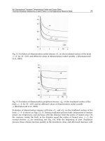
5.1 Mode boundary estimation by SVM
Before applying reinforcement learning, mode transition data are collected and used for
mode boundary estimation by SVM. Data are sampled for grid points in X, by
discretizing


21
lxlx

,,,,,


by [5, 10, 10, 10, 10, 10]. Two graphs in Fig. 13. show examples of
mode boundary estimation. In the left hand,
xx


plane is shown by fixing other variables
as l = 0.183 and


T
51,τ
by setting
0l 

. The curve in the figure shows the region where
mode 'stick' for contact point 1 and mode 'slip to negative direction of x-axis' for contact
point 2 are maintained. In the left hand,
ll



plane is shown by fixing other variables as l =
0.966 and
 
T
5255 .,.τ
by setting
0x


. The curve shows the region where mode 'slip to
positive direction of x-axis' for contact point 1 and mode `stick’ for contact point 2 are
maintained.

Fig. 13. Examples of estimated boundary by SVM

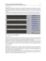
5.2 Learning of manipulation
The profile of reward per step (average) is shown in the left hand of Fig.14. Trajectories from
initial configuration to the desired one were obtained after 200 trials. It takes value of
around 6 or 7 because it is an average of one trial, in which reward of -1 is obtained at the
beginning and later reward of 10 is obtained, as far as it stays at the desired configuration.
The right hand of Fig.14 shows state value function V(s), which is calculated from action

value function by
),(max asQ
a
( s
1
and s

2
correspond to discretization of l and x, respectively).
It can be seen that the value of the desired state is the highest in the state space. 500 steps
trials are tested for 20 times. For all cases, it was possible to achieve the control to the
desired state, though numbers of trials required to achieve learning are different (around
several hundred trials).

The left hand of Fig.15 shows a trajectory obtained by the hierarchical controller with the
greedy policy. Totally five mode switching are operated to achieve desired configuration.
The right hand of Fig.15 shows the profiles of joint torques. Continuous torques are
calculated by the lower layer.

Fig. 14. Learning profile and obtained state value function

Fig. 15.Trajectory on l-x plane and joint torque profiles

Fig.16. shows contact modes δ for contact point 1 and 2. By comparing two figures, it can be
seen that when
1

= 1 (contact point 1 is slipping and the hand is moving to right),
2

= 0 (contact point 2 is stick mode and the object is stopping) holds. On the contrary, when
1

= 0 (contact point 1 is stick mode),
2

=

-
1 (contact point 2 is slipping and the object is
moving to left) holds. That is, the hand is moving together with the object. Thus, the
manipulator is switching `slipping the hand on the object to right’ mode and `moving the
object to left’ mode. Note that there are instances when both contact modes becomes stick,
that is,
0
21


. This is caused by the learning architecture, which requires stopping at
the end of each action of Q-learning. If there is no stop for each action, the total motion

Parameters for Q-learning algorithm are set as γ = 0.95, α = 0.5 and ε = 0.1. The state space is
defined as 0.620 < x < 1.440, 0 < l < 0.336(= a) and x and l axes are discretized into 6. Thus
total number of discrete states is 36. There are four actions in the upper layer Q-learning,
each corresponds to the transition to adjacent state in x, l space. Reward is defined as r(s, a)
=
),(),( arar
21
ss 
and r
1
and r
2
are specified as followings. Let
d
s
denote the goal state in
discrete state space and

1
r
is given as
 
1
10
,
0 otherwise
d
if s s
r s a





(1)
r
2
is given as
1ar
2
),(s
when constraints are broken or the hand moves out of the state
space.

5.1 Mode boundary estimation by SVM
Before applying reinforcement learning, mode transition data are collected and used for
mode boundary estimation by SVM. Data are sampled for grid points in X, by
discretizing



21
lxlx

,,,,,


by [5, 10, 10, 10, 10, 10]. Two graphs in Fig. 13. show examples of
mode boundary estimation. In the left hand,
xx


plane is shown by fixing other variables
as l = 0.183 and


T
51,τ
by setting
0l 

. The curve in the figure shows the region where
mode 'stick' for contact point 1 and mode 'slip to negative direction of x-axis' for contact
point 2 are maintained. In the left hand,
ll


plane is shown by fixing other variables as l =
0.966 and

 
T
5255 .,.τ
by setting
0x


. The curve shows the region where mode 'slip to
positive direction of x-axis' for contact point 1 and mode `stick’ for contact point 2 are
maintained.

Fig. 13. Examples of estimated boundary by SVM

5.2 Learning of manipulation
The profile of reward per step (average) is shown in the left hand of Fig.14. Trajectories from
initial configuration to the desired one were obtained after 200 trials. It takes value of
around 6 or 7 because it is an average of one trial, in which reward of -1 is obtained at the
beginning and later reward of 10 is obtained, as far as it stays at the desired configuration.
The right hand of Fig.14 shows state value function V(s), which is calculated from action

value function by
),(max asQ
a
( s
1
and s
2
correspond to discretization of l and x, respectively).
It can be seen that the value of the desired state is the highest in the state space. 500 steps
trials are tested for 20 times. For all cases, it was possible to achieve the control to the

desired state, though numbers of trials required to achieve learning are different (around
several hundred trials).

The left hand of Fig.15 shows a trajectory obtained by the hierarchical controller with the
greedy policy. Totally five mode switching are operated to achieve desired configuration.
The right hand of Fig.15 shows the profiles of joint torques. Continuous torques are
calculated by the lower layer.

Fig. 14. Learning profile and obtained state value function

Fig. 15.Trajectory on l-x plane and joint torque profiles

Fig.16. shows contact modes δ for contact point 1 and 2. By comparing two figures, it can be
seen that when
1

= 1 (contact point 1 is slipping and the hand is moving to right),
2

= 0 (contact point 2 is stick mode and the object is stopping) holds. On the contrary, when
1

= 0 (contact point 1 is stick mode),
2

=
-
1 (contact point 2 is slipping and the object is
moving to left) holds. That is, the hand is moving together with the object. Thus, the
manipulator is switching `slipping the hand on the object to right’ mode and `moving the

object to left’ mode. Note that there are instances when both contact modes becomes stick,
that is,
0
21


. This is caused by the learning architecture, which requires stopping at
the end of each action of Q-learning. If there is no stop for each action, the total motion

would be much more smooth and faster.

Fig. 16. Examples of estimated boundary by SVM

5.3 Discussion
The lower layer controller achieved local control of the manipulator using SVM boundary
obtained off-line sampling. On-line data sampling and on-line boundary estimation of the
mode boundaries will be one of our future works. On the other hand, there were some cases
where the lower layer controller could not find appropriate torques to realize desired mode.
Improvement of the lower layer controller will realize faster learning in the upper layer. One
might think that it would be much easier to learn mode boundary in
init
FF 
space using
measurement of contact force F
i
for contact point i, because the boundary can be expressed
by simple linear relation in contact force space. There are two reasons for applying
boundary estimation in the torque space: 1) In more general cases, it is not appropriate to
assume that contact forces can be always measured. E.g., in whole body manipulation
(Yoshida et al., 2006), it is difficult to measure contact force because contact can happen at

any point on the arm. 2) From the viewpoint of developing learning ability, it is also an
important learning problem to find an appropriate transformation of coordinate systems so
that boundaries between modes can be simply expressed. This will be also one of our future
works.
In order to extend the proposed framework to more useful applications such as multi-finger
object manipulation, a higher-dimensional state space should be considered. If dimension of
the state space is higher, the boundary estimation problem by SVM will require more
computational load. The problem 2) mentioned above will be a key-technique to realize a
compact and effective boundary estimation to the high-dimensional problems. The
dimension of state space for the reinforcement learning should remain low enough so that
the learning approach is applicable. Otherwise, other planning techniques might be better to
be applied.





6. Conclusion

In this chapter, we proposed two reinforcement learning approaches for object contact
robotic motion. The first approach realized a holonomic constrained motion control by
making use of a function giving a map from the general motion space to the constrained
lower dimensional one and the reward function approximation. This mapping can be
regarded as giving function approximation for the extraction of nonlinear lower
dimensional parameters. By comparing the proposed method with the ordinal
reinforcement learning method, the superiority of the proposed learning method was
confirmed. From a more general perspective, we are investigating multidimensional
mapping for broader applications. In addition, it is important to consider the continuity of
action (force control input) in the manipulation task.
In the second approach, a hierarchical approach of mode switching control learning was

proposed. In the upper layer, reinforcement learning was applied for global motion
planning. In the lower layer, SVM was applied to learn the boundaries between contact
modes and utilized to generate control input which realized mode retainment control. In
simulation, it was shown that an appropriate trajectory was obtained by reinforcement
learning with mode switching of stick/slip. For further development, fast learning of mode
boundaries will be required.

7. References

Andrew G. Barto, Steven J. Bradke & Satinder P. Singh: Learning to Act using Real-Time
Dynamic Programming, Artificial Intelligence, Special Volume: Computational
Research on Interaction and Agency, 72, 1995, pp. 81-138.Gerald Farin: Curves and
Surfaces for CAGD, Morgan Kaufmann Publishers, 2001.
Z. Gabor, Z. Kalmar, & C. Szesvari: Multi-criteria reinforcement learning, Proc. of the
15thInt. Conf. on Machine Learning, pp. 197-205, 1998.
Peter Geibel: Reinforcement Learning with Bounded Risk, Proc. of 18th Int. Conf. on
Machine Learning, pp. 162-169, 2001.
H. Kimura, T. Yamashita and S. Kobayashi, Reinforcement Learning of Walking Behaviorfor
a Four-Legged Robot, Proc. of IEEE Conf. on Decision and Control, 411-416,2001.
Cheng-Peng Kuan & Kuu-Young Young: Reinforcement Learning and Robust Control for
Robot Compliance Tasks, Journal of Intelligent and Robotic Systems, 23, pp.165-
182,1998.
O. L. Mangasarian and David R. Musicant, Lagrangian Support Vector Machines, Journal of
Machine Learning Research, 1, 161-177, 2001.
H. Miyamoto, J. Morimoto, K. Doya and M. Kawato: Reinforcement learning with via-
pointrepresentation, Neural Networks, 17, 3, 299-305, 2004.
Saleem Mohideen & Vladimir Cherkassky, On recursive calculation of the generalized
inverse of a matrix, ACM Transactions on Mathematical Software 17, Issue 1,
pp.130 - 147, 1991
J. Morimoto and K. Doya, Acquisition of stand-up behavior by a real robot using

hierarchical reinforcement learning. Robotics and Autonomous Systems 36 (1): 37-
51, 2001.

would be much more smooth and faster.

Fig. 16. Examples of estimated boundary by SVM

5.3 Discussion
The lower layer controller achieved local control of the manipulator using SVM boundary
obtained off-line sampling. On-line data sampling and on-line boundary estimation of the
mode boundaries will be one of our future works. On the other hand, there were some cases
where the lower layer controller could not find appropriate torques to realize desired mode.
Improvement of the lower layer controller will realize faster learning in the upper layer. One
might think that it would be much easier to learn mode boundary in
init
FF

space using
measurement of contact force F
i
for contact point i, because the boundary can be expressed
by simple linear relation in contact force space. There are two reasons for applying
boundary estimation in the torque space: 1) In more general cases, it is not appropriate to
assume that contact forces can be always measured. E.g., in whole body manipulation
(Yoshida et al., 2006), it is difficult to measure contact force because contact can happen at
any point on the arm. 2) From the viewpoint of developing learning ability, it is also an
important learning problem to find an appropriate transformation of coordinate systems so
that boundaries between modes can be simply expressed. This will be also one of our future
works.
In order to extend the proposed framework to more useful applications such as multi-finger

object manipulation, a higher-dimensional state space should be considered. If dimension of
the state space is higher, the boundary estimation problem by SVM will require more
computational load. The problem 2) mentioned above will be a key-technique to realize a
compact and effective boundary estimation to the high-dimensional problems. The
dimension of state space for the reinforcement learning should remain low enough so that
the learning approach is applicable. Otherwise, other planning techniques might be better to
be applied.





6. Conclusion

In this chapter, we proposed two reinforcement learning approaches for object contact
robotic motion. The first approach realized a holonomic constrained motion control by
making use of a function giving a map from the general motion space to the constrained
lower dimensional one and the reward function approximation. This mapping can be
regarded as giving function approximation for the extraction of nonlinear lower
dimensional parameters. By comparing the proposed method with the ordinal
reinforcement learning method, the superiority of the proposed learning method was
confirmed. From a more general perspective, we are investigating multidimensional
mapping for broader applications. In addition, it is important to consider the continuity of
action (force control input) in the manipulation task.
In the second approach, a hierarchical approach of mode switching control learning was
proposed. In the upper layer, reinforcement learning was applied for global motion
planning. In the lower layer, SVM was applied to learn the boundaries between contact
modes and utilized to generate control input which realized mode retainment control. In
simulation, it was shown that an appropriate trajectory was obtained by reinforcement
learning with mode switching of stick/slip. For further development, fast learning of mode

boundaries will be required.

7. References

Andrew G. Barto, Steven J. Bradke & Satinder P. Singh: Learning to Act using Real-Time
Dynamic Programming, Artificial Intelligence, Special Volume: Computational
Research on Interaction and Agency, 72, 1995, pp. 81-138.Gerald Farin: Curves and
Surfaces for CAGD, Morgan Kaufmann Publishers, 2001.
Z. Gabor, Z. Kalmar, & C. Szesvari: Multi-criteria reinforcement learning, Proc. of the
15thInt. Conf. on Machine Learning, pp. 197-205, 1998.
Peter Geibel: Reinforcement Learning with Bounded Risk, Proc. of 18th Int. Conf. on
Machine Learning, pp. 162-169, 2001.
H. Kimura, T. Yamashita and S. Kobayashi, Reinforcement Learning of Walking Behaviorfor
a Four-Legged Robot, Proc. of IEEE Conf. on Decision and Control, 411-416,2001.
Cheng-Peng Kuan & Kuu-Young Young: Reinforcement Learning and Robust Control for
Robot Compliance Tasks, Journal of Intelligent and Robotic Systems, 23, pp.165-
182,1998.
O. L. Mangasarian and David R. Musicant, Lagrangian Support Vector Machines, Journal of
Machine Learning Research, 1, 161-177, 2001.
H. Miyamoto, J. Morimoto, K. Doya and M. Kawato: Reinforcement learning with via-
pointrepresentation, Neural Networks, 17, 3, 299-305, 2004.
Saleem Mohideen & Vladimir Cherkassky, On recursive calculation of the generalized
inverse of a matrix, ACM Transactions on Mathematical Software 17, Issue 1,
pp.130 - 147, 1991
J. Morimoto and K. Doya, Acquisition of stand-up behavior by a real robot using
hierarchical reinforcement learning. Robotics and Autonomous Systems 36 (1): 37-
51, 2001.

R. Munos, A. Moore, Variable Resolution Discretization in Optimal Control, Machine
Learning, No.1, pp.1-31,2001.

J. Nakanishi, J. Morimoto, G. Endo, G. Cheng, S. Schaal, M. Kawato, Learning from
demonstration and adaptation of biped locomotion. Robotics and
AutonomousSystems 47(2-3): 79-91, 2004
S. Nakaoka, S. Hattori, F. Kanehiro, S. Kajita and H. Hirukawa, Constraint-based Dynamics
Simulator for Humanoid Robots with Shock Absorbing Mechanisms, The 2007
IEEE/RSJ International Conference on Intelligent Robots and Systems, 2007
A. van der Schaft & H. Schumacher: An Introduction to Hybrid Dynamical Systems,
Springer, 2000.
Richard S. Sutton: Dyna, an Integrated Architecture for Learning, Planning, and Reacting,
Proc. of the 7th Int. Conf. on Machine Learning, pp. 216-224, 1991.
Richard S. Sutton: Learning to Predict by the Methods of Temporal Differences, Machine
Learning, 1988, 3, 9-44.
T. Schlegl, M. Buss, and G. Schmidt, Hybrid Control of Multi-fingered Dextrous Robotic
Hands, S. Engell. G. Frehse, E. Schnieder (Eds.): Modelling, Analysis and Design of
Hybrid Systems, LNCIS 279, 437-465, 2002.
V. N. Vapnik, The Nature of Statistical Learning Theory, Springer, 1995.M. Yashima, Y.
Shiina and H. Yamaguchi, Randomized Manipulation Planning for A Multi-
Fingered Hand by Switching Contact Modes, Proc. 2003 IEEE Int. Conf. on Robotics
and Automation, 2003.
Y. Yin, S. Hosoe, and Z. Luo, A Mixed Logic Dynamical Modelling Formulation and
Optimal Control of Intelligent Robots, Optimization Engineering, Vol.8, 321-
340,2007.
E. Yoshida, P. Blazevic, V. Hugel, K. Yokoi, and K. Harada, Pivoting a Large Object: Whole-
body Manipulation by a Humanoid Robot, Applied Bionics and Biomechanics, vol.
3, no. 3, 227-235, 2006
X
Ball Control in High-speed Throwing Motion
Based on Kinetic Chain Approach

Taku Senoo*

1
, Akio Namiki*
2
and Masatoshi Ishikawa*
1

*
1
University of Tokyo, *
2
Chiba University
Japan

1. Introduction
In recent years, many robotic manipulation systems have been developed. However such
systems were designed with a primary goal of the emulation of human capabilities, and less
attention to pursuing of the upper limit in terms of speed for mechanical systems. In terms
of motor performance, there are few robots equipped with quickness. Fast movement for
robot systems provides not only improvement in operating efficiency but also new robotic
skills based on the features peculiar to high-speed motion. For example some previous
studies have been reported such as dynamic regrasping (Furukawa et al., 2006), high-speed
batting (Senoo et al., 2006) and so on. However, there is little previous work where high-
speed hand-arm coordination manipulation is achieved.
In this paper we report on experiments on the robotic throwing motion using a hand-arm
system as shown in Fig.1. First a strategy for arm control is proposed based on the "kinetic
chain" which is observed in human throwing motion. This strategy produces efficient high-
speed motion using base functions of two types derived from approximate dynamics. Next
the method of release control with a robotic hand is represented based on analysis related to
contact state during a fast swing. The release method employs features so that the apparent
force, almost all of which is generated by high-speed motion, plays a roll in robust control of

the ball direction. Finally our high-speed manipulation system is described and
experimental results are shown.


Fig. 1. Throwing motion using a hand-arm system

6

2.

In

o
n
ar
m
co
r

2.
1
W
e
j
oi
n
to
r
th
e

dr
a
ex
p
T
h
T
w
p
o
ve
l
is
ab
19
9

2.
2
Fi
g

W
e
s
w
D
O
an
th

e


N
e
in
e
th
i

Speeding Up
S

this section we
e
n
human swin
g

m
m
with rotatio
n
r
respondin
g
to a
c
1
Human Swing

e
see human mo
t
n
t in the throwi
n
r
que of triceps b
r
e
speed. Focusi
n
a
maticall
y
incre
a
p
losively radiate
h
is mechanism is
c
w
o factors are pa
r
o
wer transmissio
n
l

ocit
y
waveform

three-dimension
a
out axes, the dir
e
9
3).
2
Swing Model
a
g
. 2. Swin
g
Mod
e
e
propose a swi
n
w
in
g
model com
p
O
F and consists
o
d a coupled ben

d
e
above two fact
o

Axis-1 and axis
-
two-dimension
a

Axis-2 is per
p
interferential ac
e
xt we derive th
e
e
rtia. Gravit
y
is
a
i
s assumption th
e
S
wing Motion

e
xtract a motiona
m

otion. The prop
o
n
al
j
oints. It is
p
c
tual equipment
e

Motion
t
ion at tremend
o
ng
motion can be
r
achii, which
g
e
n
ng
on the speed

a
sed
j
ust before r
e

e
kinetic energy
c
alled "kinetic c
h
r
ticularl
y
import
a
n
(Putnam, 1993
)

is continuousl
y

m
a
l kinetic chain.

e
ctions of which
a
a
nd Its Dynamic
s
e
l
ng

model to cons
t
p
osed of the upp
o
f two revolutio
n
d
ing joint to k
e
o
rs of kinetic chai
-
3 are parallel. T
h
a
l planar model.

p
endicular to o
tion.
e
equation of mo
t
a
lso i
g
nored to c
l
e

d
y
namics doe
s
l framework for
p
o
sed swin
g
mod
e
p
ossible to con
v
e
ven if there are
d
o
us speeds in sp
o
up to 40 [rad/s
]
n
erates the elbow

or power in d
i
e
lease time. This
accumulated fro

h
ain" and it achie
v
a
nt. One is two-
d
)
. This motion h
a
m
oved from the
b
This means the
a
re different fro
m
s

t
itute the frame
w
er arm and the
l
n

j
oints , at t
h
e
ep the lower ar

m
n as described b
e
h
e state with the

ther axes. The
t
ion. To simplif
y
l
arif
y
the effect
o
s
not depend on
p
roducin
g
hi
g
h-
s
e
l can be adapte
d
v
ert model-base
d

d
ifferences in ki
n
o
rts. For example
]
(Werner, 1993).

motion, is rema
r
i
stal upper extr
e
is because a hu
m
m the early sta
g
v
es hi
g
h-speed s
w
d
imensional kin
e
a
s characteristics
b
od
y

trunk to th
e
effect of motio
n
m
each other like

w
ork of kinetic ch
a
l
ower arm. This
m
h
e shoulder and

m
horizontal. Thi
s
e
low.

elbow in extens
i
rotation about

the problem, w
e
o
f interaction bet

w
the choice of co
o
s
peed movemen
t
d
to an
y
two-lin
k
d
motion into
m
n
ematics betwee
n
the speed of an


However the ob
s
r
kabl
y
low consi
e
mit
y
, their val

u
m
an has a mecha
n
g
es of a swing
m
w
in
g
motion effi
c
e
tic chain, which
so that the peak

e
distal part. Th
e
n

g
enerated b
y
r
o
gy
ro (Mochiduk
i

a
in. Figure 2 sho
w
m
odel has a tot
a

the elbow respe
c
s
model corresp
o
i
on ( ) re
s
t
axis-2 produc
e
e
i
g
nore the mo
m
w
een
j
oints. Bec
a
o
rdinate s

y
stem,

t
based
k
robot
m
otion
n
them.

elbow
s
erved
derin
g

u
es are
n
ism to
m
otion.
c
ientl
y
.
means

of the
e
other
o
tation
i
et al.,
w
s the
a
l of 3-
c
tivel
y

o
nds to
s
ults i
n

e
s 3D
m
ent of
a
use of

so the
m

o
an

w
h
el
e

w
h

w
h
to
ot
h


2.
3
T
h
to
dr
i
ex
c

S
u

hi
g

T
o
j
oi
n
th
e

If
eq
u

w
h
ba

o
del can accom
m
d underarm pitc
h
h
ere is the
e
ments are repre
s
h

ere a
n
h
ere c
o
center of
g
ravit
y
h
er parameters b
e
3
Decompositio
n
h
e essence of the
k
distal part. Bec
a
i
ven b
y
the inter
a
c
ept for
j
oint-1;
u

ppose that
j
oint-
1
g
h-speed rotatio
n
o
obtain motion
i
n
t-3 in continuo
u
e
above assumpt
i
we express
u
ation becomes
a
h
ere and
se function repr
e
m
odate various t
y
h
. The torque
i

inertia matrix,
s
ented as
n
d .
O
o
rrespondin
g
to i
-
y
respectivel
y
. W
e
e
cause the upper

n
into Base Fun
c
k
inetic chain app
a
use in this mo
d
a
ction is desirabl
e

1
can output hi
gh
n
instantaneousl
y
i
n
j
oint-2, the ve
c
u
s uniform moti
o
i
on;
usin
g
t
h
a
second order di
are frequenc
y
,

e
sentin
g
a three-

d
y
pes of throwin
g
i
s computed as
is the cori
O
ther constant p
a
-
th link means t
h
e
assume that th
e

arm is
g
enerall
y
c
tions
roach is efficient

d
el
j
oint-1 repre
s

e
behavior for
j
oi
n
h
er power than
t
y
;
c
tor
i
o
n . The d
yn
h
e first-order ap
p
fferential equati
o

phase, and am
p
d
imensional inter
a
g
such as overha
n

o
lis and centrif
u
a
rameters are de
f
h
e mass, the entir
e
parameter incl
u

heavier tha
n
the



transmission of
p
s
ents the source

n
t-2 and joint-3.
T

t
he other

j
oints a
n

i
s substituted fo
r
n
amics of
j
oint-2


p
roximation of
t
o
n for . The sol
u

p
litude respectiv
e
a
ction of inertia
f
n
d pitch, sidear
m
ug

al force term.
f
ined as follows;


e len
g
th and the
u
din
g
is lar
ge

lower arm;
p
ower from bod
y

of power, the
m
T
herefore we set

n
d achieve stead
y
r
Eq.(5) thereb
y

s

is approximate
d
t
he Ta
y
lor seri
e
u
tion is
e
l
y
. That is an ex
f
orce.
m
pitch
(1)
Those
(2)
(3)
len
g
th
e
r than
(4)

y
trunk
m
otion


(5)
y
state
(6)
s
ettin
g

d
usin
g

(7)
e
s, this
(8)
p-type

2.

In

o
n

ar
m
co
r

2.
1
W
e
j
oi
n
to
r
th
e
dr
a
ex
p
T
h
T
w
p
o
ve
l
is
ab

19
9

2.
2
Fi
g

W
e
s
w
D
O
an
th
e


N
e
in
e
th
i

Speeding Up
S

this section we

e
n
human swin
g

m
m
with rotatio
n
r
respondin
g
to a
c
1
Human Swing

e
see human mo
t
n
t in the throwi
n
r
que of triceps b
r
e
speed. Focusi
n
a

maticall
y
incre
a
p
losivel
y
radiat
e
h
is mechanism is
c
w
o factors are pa
r
o
wer transmissio
n
l
ocit
y
waveform

three-dimension
a
out axes, the dir
e
9
3).
2

Swing Model
a
g
. 2. Swin
g
Mod
e
e
propose a swi
n
w
in
g
model com
p
O
F and consists
o
d a coupled ben
d
e
above two fact
o

Axis-1 and axis
-
two-dimension
a

Axis-2 is per

p
interferential ac
e
xt we derive th
e
e
rtia. Gravit
y
is
a
i
s assumption th
e
S
wing Motion

e
xtract a motiona
m
otion. The prop
o
n
al
j
oints. It is
p
c
tual equipment
e

Motion
t
ion at tremend
o
ng
motion can be
r
achii, which
g
e
n
ng
on the speed

a
sed
j
ust before r
e
e
kinetic ener
gy

c
alled "kinetic c
h
r
ticularl
y
import

a
n
(Putnam, 1993
)

is continuousl
y

m
a
l kinetic chain.

e
ctions of which
a
a
nd Its Dynamic
s
e
l
ng
model to cons
t
p
osed of the upp
o
f two revolutio
n
d
in

g

j
oint to k
e
o
rs of kinetic chai
-
3 are parallel. T
h
a
l planar model.

p
endicular to o
tion.
e
equation of mo
t
a
lso i
g
nored to c
l
e
d
y
namics doe
s
l framework for

p
o
sed swin
g
mod
e
p
ossible to con
v
e
ven if there are
d
o
us speeds in sp
o
up to 40 [rad/s
]
n
erates the elbow

or power in d
i
e
lease time. This
accumulated fro
h
ain" and it achie
v
a
nt. One is two-

d
)
. This motion h
a
m
oved from the
b
This means the
a
re different fro
m
s

t
itute the frame
w
er arm and the
l
n

j
oints , at t
h
e
ep the lower ar
m
n as described b
e
h
e state with the

ther axes. The
t
ion. To simplif
y
l
arif
y
the effect
o
s
not depend on
p
roducin
g
hi
g
h-
s
e
l can be adapte
d
v
ert model-base
d
d
ifferences in ki
n
o
rts. For example

]
(Werner, 1993).

motion, is rema
r
i
stal upper extr
e
is because a hu
m
m the earl
y
sta
g
v
es hi
g
h-speed s
w
d
imensional kin
e
a
s characteristics
b
od
y
trunk to th
e
effect of motio

n
m
each other like

w
ork of kinetic ch
a
l
ower arm. This
m
h
e shoulder and

m
horizontal. Thi
s
e
low.

elbow in extens
i
rotation about

the problem, w
e
o
f interaction bet
w
the choice of co
o

s
peed movemen
t
d
to an
y
two-lin
k
d
motion into
m
n
ematics betwee
n
the speed of an


However the ob
s
r
kabl
y
low consi
e
mit
y
, their val
u
m
an has a mecha

n
g
es of a swin
g

m
w
in
g
motion effi
c
e
tic chain, which
so that the peak

e
distal part. Th
e
n

g
enerated b
y
r
o
gy
ro (Mochiduk
i

a

in. Figure 2 sho
w
m
odel has a tot
a

the elbow respe
c
s
model corresp
o
i
on ( ) re
s
t
axis-2 produc
e
e
i
g
nore the mo
m
w
een
j
oints. Bec
a
o
rdinate s
y

stem,

t
based
k
robot
m
otion
n
them.

elbow
s
erved
derin
g

u
es are
n
ism to
m
otion.
c
ientl
y
.
means

of the

e
other
o
tation
i
et al.,
w
s the
a
l of 3-
c
tivel
y

o
nds to
s
ults i
n

e
s 3D
m
ent of
a
use of

so the
m
o

an

w
h
el
e

w
h

w
h
to
ot
h


2.
3
T
h
to
dr
i
ex
c

Su
hi
g

T
o
j
oi
n
th
e

If
eq
u

w
h
ba

o
del can accom
m
d underarm pitc
h
h
ere is the
e
ments are repre
s
h
ere a
n

h
ere c
o
center of
g
ravit
y
h
er parameters b
e
3
Decompositio
n
h
e essence of the
k
distal part. Bec
a
i
ven b
y
the inter
a
c
ept for
j
oint-1;
u
ppose that joint-
1

g
h-speed rotatio
n
o
obtain motion
i
n
t-3 in continuo
u
e
above assumpt
i
we express
u
ation becomes
a
h
ere and
se function repr
e
m
odate various t
y
h
. The torque
i
inertia matrix,
s
ented as
n

d .
O
o
rrespondin
g
to i
-
y
respectivel
y
. W
e
e
cause the upper

n
into Base Fun
c
k
inetic chain app
a
use in this mo
d
a
ction is desirabl
e
1
can output hi
gh
n

instantaneousl
y
i
n
j
oint-2, the ve
c
u
s uniform moti
o
i
on;
usin
g
t
h
a
second order di
are frequency,

e
sentin
g
a three-
d
y
pes of throwin
g
i
s computed as

is the cori
O
ther constant p
a
-
th link means t
h
e
assume that th
e

arm is
g
enerall
y
c
tions
roach is efficient

d
el
j
oint-1 repre
s
e
behavior for
j
oi
n
h

er power than t
y
;
c
tor
i
o
n . The d
yn
h
e first-order ap
p
fferential equati
o
phase, and am
p
d
imensional inter
a
g
such as overha
n

o
lis and centrif
u
a
rameters are de
f
h

e mass, the entir
e
parameter incl
u

heavier tha
n
the



transmission of
p
s
ents the source

n
t-2 and joint-3.
T

t
he other joints a
n

i
s substituted fo
r
n
amics of
j

oint-2


p
roximation of
t
o
n for . The sol
u

p
litude respectiv
e
a
ction of inertia
f
n
d pitch, sidear
m
ug
al force term.
f
ined as follows;


e len
g
th and the
u
din

g
is lar
ge

lower arm;
p
ower from bod
y

of power, the
m
T
herefore we set

n
d achieve stead
y
r
Eq.(5) thereb
y

s

is approximate
d
t
he Ta
y
lor seri
e

u
tion is
e
ly. That is an ex
f
orce.
m
pitch
(1)
Those
(2)
(3)
len
g
th
e
r than
(4)
y
trunk
m
otion


(5)
y state
(6)
s
ettin
g

d
usin
g

(7)
e
s, this
(8)
p-type

T
o
joi
n
th
e

If
w
so
l

w
h
ba
Al
ar
e
as

tr
a
fu
n

T
h
T
h

T
h
of
at

2.
4
Fi
g

W
e
in
c

o

o
obtain motion

o
nt-2 in continuo
u
e
above assumpt
i
w
e express
as constant, th
i
l
ution is
h
ere and
se function repr
e
thou
g
h we can
c
e
rou
g
h approxi
m

well as other u
n
aj
ectory of joint-1

n
ction as
h
e constant term
h
en the tra
j
ector
y
h
e tra
j
ector
y
of v
e
exp-t
y
pe functio
a certain time to
4
Superposition

g
. 3. Superpositio
e
s
y
nthesize th
e

c
reased as show
n
o
f base function
p
o
f
j
oint-3, the ve
c
u
s uniform moti
o
i
on;
usin
g
the firs
t
i
s equation bec
o
are frequenc
y,
e
sentin
g
the two-
d

c
alculate the freq
m
ations of the d
yn
n
known parame
t
as a sin-type ba
$\vec{c}$ is add
e

of
j
oint an
g
les is

e
locit
y
and accel
e
ns is monotonic
a
decelerate swin
g

of Base Functi
o

o
n of base functio
n
e
decomposed b
a
n
in Fi
g
.3. The ve
l
p
arameters and t
h
c
tor
o
n . The dy
t
-order approxi
m
o
mes a second
o
,
phase, and am
d
imensional kin
e
uenc

y
paramete
r
n
amics. Therefor
e
t
ers in the
n
se function. We
e
e
d to the base f
u

e
ration is the sam
a
ll
y
increasin
g
(o
r

motion.
o
ns
ns
a

se functions so
l
ocit
y
of the end
-
h
e time variable:

is substituted fo
r
y
namics of joint-3

m
ation of the Ta
y
o
rder differentia
l

plitude respecti
v
e
tic chain.
r
s by Eqs.(7)
a
e
we calculate th

e
n
ext section. In a
d
e
xpress paramet
e

u
nctions to ensur
e

e t
y
pe of functio
n
r
decreasin
g
), w
e
that the speed

-
effector is re
p

r
Eq.(5) thereb
y

s
is approximate
d
lor series and c
o
l
equation for
v
el
y
. That is a s
i
a
nd (9), these eq
u
e
frequenc
y
para
m
d
dition we also
s
e
rs concerning t
h
e
continuit
y

of
m
n
. Because the be
e
chan
g
e the si
gn


of the end-effe
c
p
resented as a f
u
s
ettin
g

d
using
(9)
o
nsider
. The
(10)
in
-type
u

ations
m
eters
s
et the
h
e base
(11)
m
otion.
(12)
havior
n
of
c
tor is
u
nction

In

E
q

Al
de
U
n
m
a

w
h
m
e
eq
u

2.
5
Fi
g



each
j
oint the
s
q
.(12) so that the
jo
thou
g
h the
j
oint

fined in a simila
r

n
der the kinema
t
a
ximize the follo
w
h
ere is a posi
t
e
ans the maxim
u
ivalent to maxi
m
,
w
5
Simulation
g
. 4. Chan
g
e of
j
o
s
tart time an
d
o
int velocit
y

equ
a

velocit
y
for exp
r
wa
y
.
t
ics constraint a
n
w
in
g
evaluation
f
t
ive definite ma
t
um and minim
u
m
izin
g
the trans
w
here is the
e

int an
g
le q2 wit
h
d
the terminatio
n
a
ls zero;
-t
y
pe functions
d
n
d d
y
namics co
n
f
unction:
t
rix, ,

u
m of the vari
a
lational kinetic
e
e
ffective mass of

t
h
respect to an
g
ul
a

n
time of the


d
oes not
g
o to z
e
n
straint, the par
a

, an
d
a
ble respectivel
y
e
ner
gy
of the en
d

t
he end-effector.

a
r velocity

swin
g
are defi
n
e
ro exactl
y
, the
t
a
meter is set s
o

d
a suffix max
o
y
. This computa
t
d
-effector motio
n

(13)

n
ed b
y

(14)
t
ime is
o
as to
(15)
o
r min
t
ion is
n
when

T
o
j
oi
n
th
e

If
w
so
l

w
h
ba
Al
ar
e
as

tr
a
fu
n

T
h
T
h

T
h
of
at

2.
4
Fi
g

W
e

in
c

o

o
obtain motion
o
n
t-2 in continuo
u
e
above assumpt
i
w
e express
as constant, th
i
l
ution is
h
ere and
se function repr
e
thou
g
h we can
c
e
rou

g
h approxi
m

well as other u
n
aj
ector
y
of
j
oint-1
n
ction as
h
e constant term
h
en the tra
j
ector
y
h
e tra
j
ector
y
of v
e
exp-t
y

pe functio
a certain time to
4
Superposition

g
. 3. Superpositi
o
e
s
y
nthesize th
e
c
reased as show
n
o
f base function
p
o
f
j
oint-3, the ve
c
u
s uniform moti
o
i
on;
usin

g
the firs
t
i
s equation bec
o
are frequenc
y,
e
sentin
g
the two-
d
c
alculate the freq
m
ations of the d
yn
n
known parame
t
as a sin-t
y
pe ba
$\vec{c}$ is add
e

of
j
oint an

g
les is

e
locit
y
and accel
e
ns is monotonic
a
decelerate swin
g

of Base Functi
o
o
n of base functio
n
e
decomposed b
a
n
in Fi
g
.3. The ve
l
p
arameters and t
h
c

tor
o
n . The d
y
t
-order approxi
m
o
mes a second
o
,
phase, and am
d
imensional kin
e
uenc
y
paramete
r
n
amics. Therefor
e
t
ers in the
n
se function. We
e
e
d to the base f
u

e
ration is the sam
a
ll
y
increasin
g
(o
r

motion.
o
ns
n
s
a
se functions so
l
ocit
y
of the end
-
h
e time variable:

is substituted fo
r
y
namics of

j
oint-3

m
ation of the Ta
y
o
rder differentia
l

plitude respecti
v
e
tic chain.
r
s by Eqs.(7)
a
e
we calculate th
e
n
ext section. In a
d
e
xpress paramet
e

u
nctions to ensur
e

e t
y
pe of functio
n
r
decreasin
g
), w
e
that the speed

-
effector is re
p

r
Eq.(5) thereb
y

s
is approximate
d
lor series and c
o
l
equation for
v
el
y

. That is a s
i
a
nd (9), these eq
u
e
frequenc
y
para
m
d
dition we also
s
e
rs concernin
g
t
h
e
continuit
y
of
m
n
. Because the be
e
chan
g
e the si
gn

of the end-effe
c
p
resented as a f
u
s
ettin
g

d
usin
g

(9)
o
nsider
. The
(10)
in
-type
u
ations
m
eters
s
et the
h
e base

(11)
m
otion.
(12)
havior
n
of
c
tor is
u
nction

In

E
q

Al
de
U
n
m
a

w
h
m
e
eq
u

2.
5
Fi
g



each
j
oint the
s
q
.(12) so that the
jo
thou
g
h the
j
oint

fined in a simila
r
n
der the kinema
t
a
ximize the follo
w
h

ere is a posi
t
e
ans the maxim
u
ivalent to maxi
m
,
w
5
Simulation
g
. 4. Chan
g
e of
j
o
s
tart time an
d
o
int velocit
y
equ
a

velocit
y
for exp
r

wa
y
.
t
ics constraint a
n
w
in
g
evaluation
f
t
ive definite ma
t
um and minim
u
m
izin
g
the trans
w
here is the
e
int an
g
le q2 wit
h
d
the terminatio
n

a
ls zero;
-t
y
pe functions
d
n
d d
y
namics co
n
f
unction:
t
rix, ,

u
m of the vari
a
lational kinetic
e
e
ffective mass of
t
h
respect to an
g
ul
a

n
time of the


d
oes not
g
o to z
e
n
straint, the par
a

, an
d
a
ble respectivel
y
e
ner
gy
of the en
d
t
he end-effector.

a
r velocity

swin

g
are defi
n
e
ro exactl
y
, the
t
a
meter is set s
o

d
a suffix max
o
y
. This computa
t
d
-effector motio
n

(13)
n
ed b
y

(14)
t
ime is

o
as to
(15)
o
r min
t
ion is
n
when

Fi
g

Fo
in
T
h
fi
g
ca
s
re
s
th
e
th
e
os
c
re

s
bo
ex
p
of
sh
a
ze
r
s
w
to
T
h

2.
6
Fi
g
g
. 5. Time respon
s
r optimization,
w
section 4.1. The
S
h
e chan
g
e in

j
oin
t
g
ure shows the c
a
s
e. In those fi
g
u
s
ult corresponds
e
d
y
namics. In a
d
e
apparent force

c
illation is attrib
u
s
ponse of
j
oint
v
th
j

oint-1 and
j
o
i
p
ressed b
y
an ex
peak time as a t
y
a
rpl
y
from the s
t
r
o althou
g
h
j
oin
t
the torqu
e
w
itches to decrea
s
. Moreo
v
h

is is as expected
6
Analogous S
w
g
. 6. Analogous
S
s
e of
j
oint veloci
t
w
e set the constr
a
S
QP method was

t
an
g
le with r
e
a
se where is c
o
res the frequen
c

to the behavior

d
dition it turns o
u

acts so that it
e
u
table to the me
c
v
elocit
y
and torq
u
i
nt-3 are express
e
p-type function.

y
pical characteris
t
t
art time .
O
t
-2 also
g
ets into
e

of
j
oint-2 decre
s
in
g
speed due t
o
v
er
j
oint-3 move
s
for a sin-t
y
pe fu
n
w
ing Model
S
win
g
Model
ty
and
j
oint torq
u
a
int usin

g
data f
r

used as the opti
m
e
spect to
j
oint v
e
o
nstant and v
a
cy
of
j
oint-2 dep
of Eq.(7), it pro
v
u
t that
j
oint-2 osc
e
xtends the arm

c
hanism of rotati
o

u
e. In the left fi
g
e
d b
y
a sin-t
y
pe

In the sin-t
y
pe t
r
t
ic of planar kin
e
O
n the other han
d
motion. This is
a
ases dramaticall
y
o
the constraint
o
s
fast despite the

n
ction.
u
e
r
om the barrett
a
m
ized calculatio
n
e
locities is
s
a
ries. The ri
g
ht fi
ends not on
b
v
es the validity
o
illates around

as in a human
o
nal
j
oints. Fi
g

u
r
g
ure it turns out


function and th
e
r
a
j
ectories we ca
n
e
tic chain. The to
r
d
the torque of
jo
a
s expected for a
n
y
. This is becau
s
o
f
j
oint an
g

les a
g

low torque of
j
o
i


a
rm, which is de
s
n
.
s
hown in Fi
g
.4.
T
g
ure shows the
r
b
ut on . Becau
s
o
f the approxima
t
. This mea
n

throwin
g
motio
n
r
e 5 represents t
h

that the tra
j
ect
o
e
tra
j
ector
y
of
j
o
i
n
observe the tra
n
r
que of
j
oint-1 in
c
o

int-2
g
raduall
y

g
n
exp-t
y
pe funct
i
s
e the motion of
g
ainst the force h
e
i
nt-3 durin
g
its
m
s
cribed
T
he left
r
everse
s
e this
t

ion of
n
s that
n
. The
h
e time
o
ries of
i
nt-2 is
n
sition
c
reases
g
oes to
i
on. At
j
oint-2
e
adin
g

m
otion.
Le
m
o

W
e
T
h

T
h

T
h
T
h
m
o
ro
t
ki
n
ax
e
W
e
li
m
Se
c

3.

In

m
e

3.
1
Fi
g

S
u
co
o
st
a

w
h
su
f

t's consider the
a
o
dels is the plac
e
e
calculate the d
y
h

e d
y
namics of
j
o
i
h
is equation is s
o
. The

h
is equation is so
l
h
e analo
gy
betw
e
o
tion. The rotati
o
t
ation about the
n
etic chain. This
e
s.
e
adopt the latte

m
ited to some e
x
c
ond, the latter
m

Control of a t
h

this section we
a
e
thod for ball co
n
1
Modeling of C
o
g
. 7. Contact mo
d
u
ppose that a ha
n
o
rdinate mo
v
a
ndard coordinat
e

h
ere m is mass
o
f
fix ’ means tha
t
a
nalo
g
ous swin
g
e
ment of
j
oint-2.
T
y
namics of this
m
i
nt-2 is approxi
m
o
lved with an ex
p

d
y
namics of
j

oi
n
l
ved with a sin-t
y
e
en the two mo
d
o
ns about paralle
l
axis which is p
e
motion oscillate
s
r model in the
e
x
tent in the for
m
m
odel requires le
s
h
rown ball
a
nal
y
ze the mode
n

trol is described
.
o
ntact State
d
el between a ha
n
n
d and a ball ar
e
v
in
g
in translat
i
e
is expresse
d
o
f the ball, r is b
a
t
the variable is

model shown i
n
T
he an
g
le bet

w
m
odel and simula
t
m
ated as
p
-type function.

n
t-3 is approxima
t
y
pe function.
d
els shows the f
o
l
axes produce a
e
rpendicular to
t
s
around the pla
n
e
xperiment for t
h
m
er model beca

u
s
s compensatin
g

t
l of the contact s
t
.

n
d and a ball
e
both ri
g
id bod
i
onal acceleratio
n
d
as
a
ll position, F is

expressed in th
e
n
Fi
g
.6. The diff

e
w
een axis-1 and
t
t
e swin
g
motion
i

The motion of
jo
t
ed as

o
llowin
g
behavi
o
planar sin-t
y
pe
k
t
he parallel axes

n
e that is perpe
n

h
e followin
g
rea
s
u
se of the const
r
t
orque for
g
ravit
y
t
ate between a h
a

ies. The equatio
n
n
and an
g
ul
a

contact force, g

e
coordinate
.

e
rence between t
h
t
he upper arm i
s
i
n a similar wa
y
.
o
int-2 oscillates
a
o
r of hi
g
h-speed

k
inetic chain. M
o

produces an ex
n
dicular to the si
s
ons. First, the s
p
r
aint of

j
oint an
g
y
than the forme
r
a
nd and a ball. N
e
n
of ball motion

a
r velocit
y

a


is
g
ravit
y
force,

.
The third term

h
e two

s
fixed.
(16)
a
round
(17)

swin
g

o
reover
p-type
n
-type
p
eed is
g
le .
r
one.
e
xt the

in the
ag
ainst
(18)

and a

is the

Fi
g

Fo
in
T
h
fi
g
ca
s
re
s
th
e
th
e
os
c
re
s
bo
ex
p
of
sh
a

ze
r
s
w
to
T
h

2.
6
Fi
g
g
. 5. Time respon
s
r optimization,
w
section 4.1. The
S
h
e chan
g
e in
j
oin
t
g
ure shows the c
a
s

e. In those fi
g
u
s
ult corresponds

e
d
y
namics. In a
d
e
apparent force

c
illation is attrib
u
s
ponse of
j
oint
v
th
j
oint-1 and
j
o
i
p
ressed b

y
an ex
peak time as a t
y
a
rpl
y
from the s
t
r
o althou
g
h
j
oin
t
the torqu
e
w
itches to decrea
s
. Moreo
v
h
is is as expected
6
Analogous S
w
g
. 6. Analogous

S
s
e of
j
oint veloci
t
w
e set the constr
a
S
QP method was

t
an
g
le with r
e
a
se where is c
o
res the frequen
c

to the behavior
d
dition it turns o
u

acts so that it
e

u
table to the me
c
v
elocit
y
and torq
u
i
nt-3 are express
e
p-type function.

y
pical characteris
t
t
art time .
O
t
-2 also
g
ets into
e
of
j
oint-2 decre
s
in
g

speed due t
o
v
er
j
oint-3 move
s
for a sin-t
y
pe fu
n
w
ing Model
S
win
g
Model
ty
and
j
oint torq
u
a
int usin
g
data f
r

used as the opti
m

e
spect to
j
oint v
e
o
nstant and v
a
cy
of
j
oint-2 dep
of Eq.(7), it pro
v
u
t that
j
oint-2 osc
e
xtends the arm

c
hanism of rotati
o
u
e. In the left fi
g
e
d b
y

a sin-t
y
pe

In the sin-t
y
pe t
r
t
ic of planar kin
e
O
n the other han
d
motion. This is
a
ases dramaticall
y
o
the constraint
o
s
fast despite the

n
ction.
u
e
r
om the barrett

a
m
ized calculatio
n
e
locities is
s
a
ries. The ri
g
ht fi
ends not on
b
v
es the validit
y

o
illates around

as in a human
o
nal
j
oints. Fi
g
u
r
g
ure it turns out

function and th
e
r
a
j
ectories we ca
n
e
tic chain. The to
r
d
the torque of
jo
a
s expected for a
n
y
. This is becau
s
o
f
j
oint an
g
les a
g

low torque of

j
o
i


a
rm, which is de
s
n
.
s
hown in Fi
g
.4.
T
g
ure shows the
r
b
ut on . Becau
s
o
f the approxima
t
. This mea
n
throwin
g
motio
n

r
e 5 represents t
h

that the tra
j
ect
o
e
tra
j
ector
y
of
j
o
i
n
observe the tra
n
r
que of
j
oint-1 in
c
o
int-2
g
raduall
y

g
n
exp-t
y
pe funct
i
s
e the motion of
g
ainst the force h
e
i
nt-3 durin
g
its
m
s
cribed
T
he left
r
everse
s
e this
t
ion of
n
s that
n

. The
h
e time
o
ries of
i
nt-2 is
n
sition
c
reases
g
oes to
i
on. At
j
oint-2
e
adin
g

m
otion.
Le
m
o
W
e
T
h

T
h

T
h
T
h
m
o
ro
t
ki
n
ax
e
W
e
li
m
Se
c

3.

In

m
e

3.
1
Fi
g

S
u
co
o
st
a

w
h
su
f

t's consider the
a
o
dels is the plac
e
e
calculate the d
y
h
e d
y
namics of
j

o
i
h
is equation is s
o
. The

h
is equation is so
l
h
e analo
gy
betw
e
o
tion. The rotati
o
t
ation about the
n
etic chain. This
e
s.
e
adopt the latte
m
ited to some e
x
c

ond, the latter
m

Control of a t
h

this section we
a
e
thod for ball co
n
1
Modeling of C
o
g
. 7. Contact mo
d
u
ppose that a ha
n
o
rdinate mo
v
a
ndard coordinat
e
h
ere m is mass
o
f

fix ’ means tha
t
a
nalo
g
ous swin
g
e
ment of
j
oint-2.
T
y
namics of this
m
i
nt-2 is approxi
m
o
lved with an ex
p

d
y
namics of
j
oi
n
l
ved with a sin-t

y
e
en the two mo
d
o
ns about paralle
l
axis which is p
e
motion oscillate
s
r model in the
e
x
tent in the for
m
m
odel requires le
s
h
rown ball
a
nal
y
ze the mode
n
trol is described
.
o
ntact State

d
el between a ha
n
n
d and a ball ar
e
v
in
g
in translat
i
e
is expresse
d
o
f the ball, r is b
a
t
the variable is

model shown i
n
T
he an
g
le bet
w
m
odel and simula
t

m
ated as
p
-type function.

n
t-3 is approxima
t
y
pe function.
d
els shows the f
o
l
axes produce a
e
rpendicular to
t
s
around the pla
n
e
xperiment for t
h
m
er model beca
u
s
s compensatin
g

t
l of the contact s
t
.

n
d and a ball
e
both ri
g
id bod
i
onal acceleratio
n
d
as
a
ll position, F is

expressed in th
e
n
Fi
g
.6. The diff
e
w
een axis-1 and
t

t
e swin
g
motion
i

The motion of
jo
t
ed as

o
llowin
g
behavi
o
planar sin-t
y
pe
k
t
he parallel axes

n
e that is perpe
n
h
e followin
g
rea

s
u
se of the const
r
t
orque for
g
ravit
y
t
ate between a h
a

ies. The equatio
n
n
and an
g
ul
a

contact force, g

e
coordinate
.
e
rence between t
h
t

he upper arm i
s
i
n a similar wa
y
.
o
int-2 oscillates
a
o
r of hi
g
h-speed

k
inetic chain. M
o

produces an ex
n
dicular to the si
s
ons. First, the s
p
r
aint of
j
oint an
g
y

than the forme
r
a
nd and a ball. N
e
n
of ball motion

a
r velocit
y

a


is
g
ravit
y
force,

.
The third term

h
e two
s
fixed.
(16)
a

round
(17)

swin
g

o
reover
p-type
n
-type
p
eed is
g
le .
r
one.
e
xt the

in the
ag
ainst
(18)

and a

is the

in

e
te
r
ro
t
n
o
T
h
S
u
th
e
co
o
T
h


Si
n
co
n

T
h
su
b

Si

m

T
h
w
e

e
rtia force due t
o
r
m is the centrif
u
t
ator
y
motion, E
q
on
-inertial s
y
ste
m
h
e motion of the
h
i. The hand
g
ii. The conta
c

certain tim
e
iii. The two fi
n
the fingers.

u
ppose that the x
-
e
plane o
f
the tw
o
o
rdinates as sho
w
h
e condition whe
r
without slidin
g
i
s
n
ce the ball can
n
n
ditions are satis
h

e d
y
namics of
b
stituted for Eq.
(
m
ilarl
y
, the nor
m
h
e ball is release
d
e
anal
y
zed the re
l
o
accelerated m
o
ug
al force. Sinc
e
q
.(18) contains t
h
m
.

h
and is set to thr
o
g
rasps the ball wi
t
c
t state is switc
h
e
.
ng
ers move in th
e

-
axis is set alon
g

o
fin
g
ers, and th
e
w
n in Fi
g
.7.
r
e the ball with

r
s
represented as

n
ot be moved i
n
fied:
rollin
g
motion
(
18):
m
al force is co
m
d
from the fin
g
er
s
l
ation between t
h
o
tion, the fourth
t
e
the throwi
n

g

m
h
e considerable e
o
w a ball b
y
follo
w
t
h three fin
g
ers s
o
h
ed to two-fin
g
e
r
e
same wa
y
and
r
the two fin
g
ers f
o
e

z-axis is set so
t
r
adius a and mo
m
n
the y-axis and
is calculated a
s
m
puted as
s
when the nor
m
h
e normal force a
n
t
erm is the Cori
o
m
otion includes
ffect of the appa
w
in
g
three steps.
o
as not to drop i
r

contact b
y
rel
e
r
elease the ball
w
o
r release, the y-
a
t
hat the three ax
e
m
ent of inertia

z
-axis until rele
a

s
follows when


m
al force is reduc
e
n
d the motion of

o
lis force, and t
h
three dimensio
n
rent force peculi
a

t until a
g
iven ti
m
e
asin
g
one fin
ge
w
hile the ball roll
s
a
xis is perpendic
u
e
s constitute orth
o
rolls at
a
se time, the fol
l

Eqs.(19) and (
2
e
d to zero or les
s

rollin
g
.

h
e fifth
n
al fast
a
r to a
m
e.
e
r at a
s
alon
g

u
lar to
og
onal
an
g

les
(19)
l
owin
g

(20)
2
0) are
(21)
(22)
s
. Then
Fi
g

Fi
g
D
e
ca
n
w
i
T
h
ro
l
be
c

sp
e

3.
2
Fi
g

T
h

w
h
.
T
an

g
. 8. Relation bet
w
g
ure 8 shows t
h
e
pendin
g
on the
c
n
roll in either t

h
i
thout the effect
o
h
e faster the man
i
l
lin
g
distance c
a
c
ause the motio
n
e
ed of rolling. T
h
2
Released Ball
g
. 9. Rollin
g
effec
t
h
e velocit
y
of the
b

h
ere is transl
a
. If the rollin
g
d
i
T
hat is, throwin
g

d rollin
g
velocit
y
w
een normal for
c
h
e rollin
g
dista
n
c
onditions of the

h
e positive or ne
g
o

f a normal forc
e
i
pulator moves,
t
a
nnot be drama
t
n
time becomes s
h
h
erefore we assu
m
Motion
t
for control of t
h
b
all expressed in

a
tional velocit
y
o
f
i
stance is short, t
h
direction depen

d
y
of the ball.
c
e and rollin
g
dis
t
n
ce and the no

acceleration and

g
ative direction,
o
e
as soon as the
g
t
he lon
g
er
g
ener
a
t
icall
y
increased.

h
ort until release

m
e that the ball i
s
h
rowin
g
directio
n

standard coordi
n
f
the end-effecto
r
h
e above equatio
n
d
s mainl
y
on the
t
t
ance
r
mal force und
e

the posture of t
h
o
r the hand som
e
g
raspin
g
fin
g
er is

a
ll
y
the rollin
g
d
i
It is onl
y
a fe
w

of the ball, whil
e
s
released before
i

n

n
ates is calculate
d

r
, and R is a rot
a
n
can be approxi
m
t
ranslational vel
o

e
r var
y
in
g
con
d
h
e manipulator, t
h
e
times releases t
h

released from t
h
i
stance is. Howe
v
w
centimeters.
T
e
fast motion bri
n
i
t rolls to the fin
g
d
as follows:
a
tion matrix fro
m
m
ated as
o
cit
y
of the end-
e
d
itions.
h
e ball

h
e ball
h
e ball.
v
er the
T
his is
ng
s fast
g
ertip.

(23)
m
to
e
ffector

in
e
te
r
ro
t
n
o
T
h
S

u
th
e
co
o
T
h


Si
n
co
n

T
h
su
b

Si
m

T
h
w
e

e
rtia force due t
o

r
m is the centrif
u
t
ator
y
motion, E
q
on
-inertial s
y
ste
m
h
e motion of the
h
i. The hand
g
ii. The conta
c
certain tim
e
iii. The two fi
n
the fingers.

u
ppose that the x
-
e

plane o
f
the tw
o
o
rdinates as sho
w
h
e condition whe
r
without slidin
g
i
s
n
ce the ball can
n
n
ditions are satis
h
e d
y
namics of
b
stituted for Eq.
(
m
ilarl
y
, the nor

m
h
e ball is release
d
e
anal
y
zed the re
l
o
accelerated m
o
ug
al force. Sinc
e
q
.(18) contains t
h
m
.
h
and is set to thr
o
g
rasps the ball wi
t
c
t state is switc
h
e

.
ng
ers move in th
e

-
axis is set alon
g

o
fin
g
ers, and th
e
w
n in Fi
g
.7.
r
e the ball with
r
s
represented as

n
ot be moved i
n
fied:
rollin
g

motion
(
18):
m
al force is co
m
d
from the fin
g
er
s
l
ation between t
h
o
tion, the fourth
t
e
the throwi
n
g

m
h
e considerable e
o
w a ball b
y
follo
w

t
h three fin
g
ers s
o
h
ed to two-fin
g
e
r
e
same wa
y
and
r
the two fin
g
ers f
o
e
z-axis is set so
t
r
adius a and mo
m
n
the y-axis and
is calculated a
s
m

puted as
s
when the nor
m
h
e normal force a
n
t
erm is the Cori
o
m
otion includes
ffect of the appa
w
in
g
three steps.
o
as not to drop i
r
contact b
y
rel
e
r
elease the ball
w
o
r release, the y-
a

t
hat the three ax
e
m
ent of inertia

z
-axis until rele
a

s
follows when


m
al force is reduc
e
n
d the motion of

o
lis force, and t
h
three dimensio
n
rent force peculi
a

t until a
g

iven ti
m
e
asin
g
one fin
ge
w
hile the ball roll
s
a
xis is perpendic
u
e
s constitute orth
o
rolls at
a
se time, the fol
l
Eqs.(19) and (
2
e
d to zero or les
s

rollin
g
.

h
e fifth
n
al fast
a
r to a
m
e.
e
r at a
s
alon
g

u
lar to
og
onal
an
g
les
(19)
l
owin
g

(20)
2
0) are
(21)

(22)
s
. Then
Fi
g

Fi
g
D
e
ca
n
w
i
T
h
ro
l
be
c
sp
e

3.
2
Fi
g

T
h

w
h
.
T
an

g
. 8. Relation bet
w
g
ure 8 shows t
h
e
pendin
g
on the
c
n
roll in either t
h
i
thout the effect
o
h
e faster the man
i
l
lin
g

distance c
a
c
ause the motio
n
e
ed of rolling. T
h
2
Released Ball
g
. 9. Rollin
g
effec
t
h
e velocit
y
of the
b
h
ere is transl
a
. If the rollin
g
d
i
T
hat is, throwin
g

d rollin
g
velocit
y
w
een normal for
c
h
e rollin
g
dista
n
c
onditions of the

h
e positive or ne
g
o
f a normal forc
e
i
pulator moves,
t
a
nnot be drama
t
n
time becomes s

h
h
erefore we assu
m
Motion
t
for control of t
h
b
all expressed in

a
tional velocit
y
o
f
i
stance is short, t
h
direction depen
d
y
of the ball.
c
e and rolling dis
t
n
ce and the no

acceleration and

g
ative direction,
o
e
as soon as the
g
t
he lon
g
er
g
ener
a
t
icall
y
increased.
h
ort until release

m
e that the ball i
s
h
rowin
g
directio
n

standard coordi
n
f
the end-effecto
r
h
e above equatio
n
d
s mainl
y
on the
t
t
ance
r
mal force und
e

the posture of t
h
o
r the hand som
e
g
raspin
g
fin
g
er is

a
ll
y
the rollin
g
d
i
It is onl
y
a fe
w

of the ball, whil
e
s
released before
i
n

n
ates is calculate
d

r
, and R is a rot
a
n
can be approxi
m

t
ranslational vel
o

e
r var
y
in
g
con
d
h
e manipulator, t
h
e
times releases t
h

released from t
h
i
stance is. Howe
v
w
centimeters.
T
e
fast motion bri
n
i

t rolls to the fin
g
d
as follows:
a
tion matrix fro
m
m
ated as
o
cit
y
of the end-
e
d
itions.
h
e ball
h
e ball
h
e ball.
v
er the
T
his is
ng
s fast
g
ertip.

(23)
m
to
e
ffector

3.
3
B
a
re
l
g
r
e
H
o
is
pr
o
th
e
W
e
at
th
e
co
n

W
e
tr
a

T
h
T
h
ve
l
is
n
th
e
co
n

4.

4.
1
Fi
g

T
h
m
a

re
v
ef
f
3
Strategy for B
a
a
sed on the abo
v
l
ease timin
g
and

e
atl
y
affected b
y
o
wever it is diffi
c
difficult to pos
i
o
pose a strategy
e
throwin
g

direc
t
e
control the ha
n
the same time.
B
e
normal force is
n
trolled to releas
e
control the han
aj
ector
y
at releas
e
h
e rollin
g
accel
e
h
erefore the ball r
l
ocit
y
of the fin
ge

not released at t
h
e
release directi
o
n
trol of the ball i
s

Experiments

1
System Confi
g
g
. 10. High-spee
d
h
e arm is a wir
e
a
nipulator is sh
o
v
olution and be
n
f
ector of 6 [m/s]
a
a

ll Control
v
e results, two el

the other is co
n

the translationa
l
c
ult to control th
e
i
tivel
y
appl
y
th
e

for ball control i
t
ion.
n
d so that release

B
ecause both roll
i
represented as

e the ball when t
h
d so that the ball
e
point. This con
d
e
ration near rel
e
olls toward dist
a
e
r
j
ust after rele
a
h
e desired relea
s
o
n of the ball to
s
achieved.
g
uration
d
manipulator s
ys
e
-drive manipul

a
o
wn in Fi
g
.10(a)
.
n
din
g
motion. Hi
g
a
nd maximum a
c
ements are imp
o
n
trol of the direc
t
l
acceleration an
d
e
se variables in p
a
e
rolli
n
g
motio

n
i
n which the roll
i

of
g
raspin
g
fin
g
i
n
g
distant and
r
b
y
h
e followin
g
con
d
is released in th
e
d
ition of control i
s
e
ase point is e

x
a
l direction of the

a
se is b
y

E
s
e time due to so
ward the tar
g
et

s
tem
a
tor (Barrett Te
c
.
The manipulat
o
g
h-speed move
m
c
celeration of 58 [
o
rtant to ball co

n
t
ion of release.
T
d
the translation
a
a
rallel with hi
g
h
n
to directional
i
ng motion acts
s
er and release of

r
ollin
g
velocit
y
a

Eq.(22). Therefo
r
d
ition is satisfied

e
tan
g
ential dire
c
s
represented as


x
pressed as

fin
g
er if
E
q.(25). This resu
l
me errors, the r
o

as shown in Fi
g
c
hnolo
gy
Inc.).
T
o
r has 4-DOF c

o
m
ent with maxim
u
m/s
2
] is achieve
d
n
trol. One is co
n
T
hese two eleme
n
a
l velocit
y
respe
c
accurac
y
. In add
control. Theref
o
s
econdarily to m
a

the ball are perf
a

re zero at releas
e
r
e the
g
raspin
g
fi
n
d
;
c
tion of the end-
e
b
y

E
. On the other h
a
l
t means that if t
h
o
lling of the ball
g
.9. As a result

T
he kinematics

o
nsistin
g
of alte
r
u
m velocit
y
of t
h
d
.
n
trol of
n
ts are
c
tivel
y
.
ition it
o
re we
a
intain
ormed
e
time,
ng
er is

(24)
e
ffector
(25)
E
q.(21).
a
nd the
h
e ball
affects
robust
of the
r
natel
y

h
e end-
T
h
dr
i
T
h
th
a
0.
1
Fi

g

4.
2
T
h
di
s
tr
a
be
t
en
a
th
a
co
m


4.
3
Fi
g

Fi
g
di
r
T

h
j
oi
n
fi
g
si
m
In
as

It
fi
n
T
h
ca
l
A
c
ex
p

h
e hand consists
i
ve
g
ear and a hi
g

h
e desi
g
n of this
a
a
n rated power
o
1
[s]. Its maximu
m
g
ure 10(b) shows

2
Experimental
S
h
e manipulator t
h
s
tance. The tar
ge
a
nsformed to the

t
ween mechanis
m
a

ble accurate co
n
a
t Eq.(5) is satisfi
e
m
puted torque
m
3
Experimental
R
g
. 11. Experimen
t
g
ure 11(a) shows

r
ection oscillates
h
e time response
n
t-3 correspond
g
ure also indicat
e
m
ple controller e
x
Fi

g
.12and Fig.13
,

a continuous se
q
turns out that
g
ng
ers, and then t
h
h
e success rate
w
l
ibration of the
gr
c
cordin
g
l
y
, a tac
p
erimental resul
t
of three fin
g
ers
g

h-power mini a
c
a
ctuator is based
o
utput, should b
e
m
velocit
y
is 300
[

the hand-arm s
y
S
etting
h
rew a urethane

e
t is a net with

one correspond
i
m
s. In addition
w
n
trol of hi

g
h-spe
e
e
d, this simple c
o
m
ethod;
R
esult
t
al data of manip
u

the tra
j
ector
y
of
t
around the hei
gh
of
j
oint velocitie
s
to a sin-t
y
pe m
o

e
s that accurate
x
cept the oversh
o
,
the chan
g
e in c
o
q
uence of picture
g
raspin
g
state w
i
h
e ball is thrown
t
w
as about 40 %
r
aspin
g
state and
tile or force fee
d
t
s are shown as a

and a wrist. It
h
c
tuator are fitted

on the new conc
e
e
improved. The
h
[
rpm], and the m
a
stem.

ball with radiu
s
radius 10 [cm].

i
n
g
to the arm s
h
w
e adopted a
g
ra
v

e
d movement. B
e
o
ntroller pla
y
s a
n
u
lator motio
n

t
he end-effector.

h
t of the elbow.
T
s
is shown in Fi
g
o
de while
j
oint-2

control on fast
s
o
ot of

j
oint-1.
o
ntact state and t
h
s taken at interv
a
i
th three fin
g
ers

t
oward the tar
g
e
t
. Failure was c
a
nonuniform def
o
d
back control
w

movie on the fol
l
h
as 10-DOF in t
o

in each fin
g
er li
n
e
pt that maximu
m
h
and can close it
s
a
ximum output i
s
5 [cm] toward
s

The d
y
namics
o
h
own in Fi
g
.10(
a
v
it
y
-compensate

d
e
cause the swin
g
n
equivalent role
a

It turns out that
t
T
his is caused b
y
g
.10(b). It turns o
u
corresponds to
a
s
win
g
motion is

h
e tra
j
ector
y
o
f

a

a
ls of 100 [ms] a
n

is switched to
t
.
a
used mainl
y
b
y
o
rmatio
n
of a ba
l
w
ould improve t
h
l
owin
g
web site.

o
tal. A small ha
r

n
k (Namiki et al.
,
m
power output,

s

j
oints at 180 [d
e
s 12 [N].
s
the tar
g
et fro
m
o
f the swin
g
m
o
a
) due to the dif
f
d
PD controller s

motion is
g

ener
a
a
s well as follow
i


t
he motion in th
e
y
the exp-t
y
pe fu
n
u
t that both
j
oin
t
a
n exp-t
y
pe mo
d

achieved even
b

thrown ball are

s
n
d 66 [ms] respe
c
release state wi
t
y
uncertaint
y
in
l
l due to
g
raspin
g
h
e success rate.

r
monic
,
2003).

rather
eg
] per
m
3 [m]
o
del is

f
erence
o as to
a
ted so
i
n
g
the
(26)
e
z-axis
n
ction.
t
-1 and
d
e. The
by
the
s
hown
c
tivel
y
.
t
h two
initial
g

force.

These