Robotics 2 E Part 13 doc
Bạn đang xem bản rút gọn của tài liệu. Xem và tải ngay bản đầy đủ của tài liệu tại đây (996.33 KB, 30 trang )
350
Manipulators
FIGURE
9.23f)
Idea
of a
"trunk" made
of
Stewart-platform-like
elements.
This
idea
belongs
to Dr. A. Sh.
Kiliskor.
9.4
Grippers
In
previous sections
we
have discussed
the
kinematics
and
dynamics
of
manipu-
lators.
Now let us
consider
the
tool that manipulators mainly
use—the
gripper.
To
manipulate,
one
needs
to
grip
and
hold
the
object being manipulated. Grippers
of
various natures exist.
For
instance, ferromagnetic parts
can be
held
by
electromag-
netic grippers. This gripping device
has no
moving parts
(no
degrees
of
freedom
and
no
drives).
It is
easily controlled
by
switching
the
current
in the
coil
of the
electro-
magnet
on or
off. However,
its use is
limited
to the
parts' magnetic properties,
and
magnetic
forces
are
sometimes
not
strong enough. When relatively large sheets
are
handled, vacuum suction cups
are
used;
for
instance,
for
feeding
aluminum, brass,
steel,
etc.,
sheets into stamps
for
producing
car
body parts. Glass sheets
are
also handled
in
this way,
and
some printing presses
use
suction cups
for
gripping paper sheets
and
introducing them into
the
press. Obviously,
the
surface
of the
sheet must
be
smooth
enough
to
provide reliability
of
gripping
(to
seal
the
suction
cup and
prevent leakage
of
air and
loss
of
vacuum).
Here, also,
no
degrees
of
freedom
are
needed
for
gripping.
The
vacuum
is
switched
on or
off
by an
automatically controlled valve.
(We
illustrated
the use of
such suction cups
in the
example shown
in
Figure
2.10.)
Grippers
essentially replace
the
human hand.
If
the
gripping abilities
of a
mechan-
ical
five-finger
"hand"
are
denoted
as
100%,
then
a
four-finger
hand
has 99% of its
ability,
a
three-finger
hand about 90%,
and a
two-finger
hand 40%.
We
consider here some designs
of
two-fingered grippers.
In the
gripper shown
in
Figure
9.24,
piston
rod 1
moves
two
symmetrically
attached
connecting
links
2
which
in
turn move gripping levers
3,
which have jaws
4.
(Cylinder
5 can
obviously
be
replaced
by
any
other drive: electromagnet, cable wound
on a
drum driven
by a
motor, etc.)
The
jaws shown here
are
suitable
for
gripping cylindrical bodies having
a
certain range
of
diameters. Attempts
to
handle other shapes
or
sizes
of
parts
may
lead
to
asymmet-
rical
gripping
by
this device, because
the
angular displacements
of
jaws
may not be
parallel.
To
avoid skewing
in the
jaws, solutions like those shown
in
Figure 9.25a)
or
b)
are
used.
In
Case
a) a
simple cylinder
1
with piston
2 and
jaws
3
ensures parallel
9.4
Grippers
351
FIGURE
9.24
Design
of a
simple
mechanical
gripper.
FIGURE
9.25
Grippers
with
translational
jaw
motion.
displacement
of the
latter.
In
case
b) a
linkage
as in
Figure 9.24,
but
with
the
addition
of
connecting rods
6 and
links
7
with attached jaws
4,
provides
the
movement needed.
These additional elements create parallelograms which provide
the
transitional move-
ment
of the
jaws.
Various
other mechanical designs
of
grippers
are
possible.
For
instance, Figure 9.26
shows possible solutions
a) and b)
with angular movement
of
jaws
1,
while cases
c)
and d)
provide parallel displacement
of
jaws
1. In all
cases
the
gripper
is
driven
by rod
2.
All the
cases presented
in
Figure 9.26 possess rectilinear kinematic pairs
3.
Intro-
duction
of
higher-degree
kinematic pairs
are
shown
in
Figure 9.27.
In
case
a) cam 1
fastened
on rod 2
moves levers
3 to
which jaws
4 are
attached. Spring
5
ensures
the
contact between
the
levers
and the
cam.
In
case
b) the
situation
is
reversed: cams
1
are
fastened
onto
levers
3 and rod 2
actuates
the
cams,
thus
moving jaws
4.
Spring
5
closes
the
kinematic chain.
In
case
c),
which
is
analogous
to
case
b),
springs
5
also play
the
role
of
joints.
In
case
d) the
higher-degree kinematic pair
is a
gear set.
Rack
1
(moved
by
rod 2) is
engaged with gear sector
3
with jaws
4
attached
to
them.
Cases
a) to d)
have dealt with angular displacement
of
jaws.
In
case
e) we see how the
addition
of
parallelograms
5 (as in the
example
in
Figure
9.25b))
to the
mechanism shown
in
Figure
9.27d)
makes
the
motion
of the
jaws translational.
The
last
two
cases
do not
need
springs, since
the
chain
is
closed kinematically.
352
Manipulators
FIGURE
9.26
Designs
of
grippers using low-degree kinematic pairs.
FIGURE
9.27
Designs
of
grippers using high-degree
kinematic
pairs.
9.4
Grippers
353
To
describe these mechanisms quantitatively
we use the
relationships between:
1.
Forces
F
G
which
the
jaws develop,
and the
force
F
d
which
the
driving
rod
applies;
and
2.
The
displacements
S
d
of the
driving
rod and the
jaws
of the
gripper
S
G
.
Figure
9.28 illustrates
these
parameters
and
graphically shows
the
functions
S
G
(S
d
)
and
F
G
/Fd=flSj
for
a
gripper.
This
discussion
of
grippers
has
been influenced
by the
paper
by J.
Volmer,
"Tech-
nische Hochschule
Karl-Marx-Stadt,
DDR, Mechanism
fur
Greifer
von
Handhaberg-
eraten,"
Proceedings
of the
Fifth
World
Congress
on
Theory
of
Machines
and
Mechanisms, 1979,
ASME.
We
should note
that
the
examples
of
mechanical grippers
discussed above permit
a
certain degree
of flexibility in the
dimensions
of
parts
the
gripper
can
deal with. This property allows using these grippers
for
measuring.
For
instance,
by
remembering
the
values
of
S
d
by
which
the
driving
rod
moves
to
grip
the
parts,
the
system
can
compare
the
dimensions
of the
gripped parts.
When
the
manipulated parts
are
relatively small
and
must
be
positioned accurately,
miniaturization
of the
gripper
is
required.
A
solution
of the
type shown
in
Figure 9.29
can be
recommended,
for
example,
in
assembly
of
electronic circuits. Here,
the
gripper
FIGURE
9.28
Characteristics
of a
mechanical
gripper.
354
Manipulators
is
a
one-piece tool made
of
elastic material that
can
bend
and
surround
the
gripped
part,
of
diameter
d, to
create
frictional
force
to
hold
the
part,
and
then
to
release
it
when
it is
fastened
on the
circuit board.
The
overlap
h
=
Q.2d
serves this purpose.
Three-fingered
grippers
are
also available
(or can be
designed
for
special
purposes).
Figure
9.30 shows
a
concept
of a
three-fingered
gripper. Part
a)
presents
a
general view
and
part
b)
shows
a
side
view.
Here,
1 is the
base
of the
gripper
and 2 the
driving rod,
which
is
connected
by
joints
and
links
to fingers 3.
When
rod 2
moves right,
the fingers
open,
and
when
it
moves
left,
they close. This gripper
(as
well
as
some considered
earlier)
can
grip
a
body
from
both
the
outside
and the
inside. (Such grippers
are
pro-
duced
by
Mecanotron Corporation, South
Plainfield,
New
Jersey,
U.S.A.)
One
of the
most serious problems
that
appears
in
manipulators equipped with dif-
ferent
sorts
of
grippers
is
control
of the
grasping
force
the
gripper develops. Obviously,
there must
be
some
difference
between grasping
a
metal blank,
a
wine glass,
or an
egg,
even when
all
these objects
are the
same size. This
difference
is
expressed
in the
dif-
ferent
amounts
of
force
needed
to
hold
the
objects
and
(what
is
more important)
the
limited pressure allowed
to be
applied
to
some objects. Figure 9.31 shows
a
possible
solution
for
handling tender, delicate objects. Here, hand
1 is
provided with
two
elastic
FIGURE
9.30 Three-fingered
gripper.
FIGURE
9.31
A
soft
gripper
for
grasping
delicate
objects.
9.4
Grippers
355
pillows
2.
When
inflated
by a
controlled pressure, they develop enough
force
to
hold
the
glass, while keeping
the
pressure
on it
small enough
to
prevent damage. (The small
pressure creates considerable holding
force
due to the
relatively large contact area
between
the
glass
and the
pillows.)
It is a
satisfying
solution when modest accuracy
of
positioning
is
sufficient.
A
more sophisticated approach
to the
problem
of
handling delicate objects
is the
Utah-MIT
dextrous hand which
is
described
in the
Journal
of
Machine
Design
of
June
26,
1986. This
is a
four-fingered
hand
consisting
of
three
fingers
with
four
degrees
of
freedom
and one
"thumb" with
four
degrees
of
freedom.
The
"wrist"
has
three degrees
of
freedom.
The
thumb acts against
the
three
fingers.
Thus,
the
hand
consists
of 16
movable links driven
by a
system
of
pneumatically operated "tendons"
and 184
low-
friction
pulleys.
The
joints connecting
the
links include precision bearings.
The
problem
of
air
compressibility
is
overcome
by use of
special control valves.
Figure
9.32a)
shows
a
general design
of one finger.
Here links
A, B, and C can
rotate around their joints.
The
space
inside
the
links
is
hollow
and
contains
the
pulleys
and the
tendons,
which
go
around
the
pulleys
and are
fastened
to the
appropriate links. Figure
9.32b)
shows
the
drive
of
link
C.
Tendons
I and
la
run
around pulleys
7, 8, and 9 and are
fastened
to
the
center
of
pulley
6.
Thus, pulling tendons
I and
la
causes bending
and
straighten-
ing of
link
C.
Figure
9.32c)
shows
the
control
of
link
B by
tendons
II and
Ha,
and
Figure
9.32d)
shows
the
control
of
link
A by
tendons
III and
Ilia.
A
pair
of
tendons
IV and
IVa
are
used
for
turning
the
whole
finger
around
the
X-Xaxis,
as
shown
in
Figure
9.32e).
The
Utah-MIT
hand
has 16
position
sensors
and 32
tendon-tension
sensors.
Thus
its
grasping
force
can be
controlled,
and the
object handled
by the
gripper with
a
light
or
heavy
touch.
For
simpler grippers
(as in
Figures 9.24, 9.28,
and
9.30),
force-sensitive
jaws
can be
made
as
shown
in
Figure 9.33. Here, part
1 is
grasped
by
jaws
2
which develop grasp-
ing
force
F
G
.
The
force
is
measured
by
sensor
3
located
in
base
4
which connects
the
gripper
with drive
rod 5. The
latter moves rack
6 and the
kinematics
of the
gripper.
Force
F
d
,
which
is
developed
by rod 5,
determines
grasping
force
F
G
.
Sensor
3
enables
the
desired ratio
F
G
/F
d
to be
achieved.
The
sensor
can be
made
so as to
measure more
than
one
force,
say, three projections
offerees
and
torques relative
to a
coordinate axis.
These devices help
to
control
the
grasping
force;
however,
its
value must
be
pre-
determined
(before
using
the
gripper)
and the
system tuned appropriately. Serious
efforts
are
being devoted
to
simulating
the
behavior
of a
human hand, which "knows"
how to
learn
the
required grasping
force
during
the
grasping process
itself.
This ability
of
a
live
hand
is due to its
tactile sensitivity.
Next,
we
consider some concepts
of
arti-
ficial
tactile sensors installed inside
the
gripper's
fingers or
jaws. Figure 9.34 illustrates
a
design
for a
one-dimensional tactile sensor.
laws
1
develop grasping
force
F
G
which
must cause enough
frictional
force
F
u
(vertically directed)
to
prevent
object
2
from
falling
due to
gravitational
force
P. The
sensor consists
of
roller
3
mounted
on
shaft
4
by
means
of
bearings.
Shaft
4 is
mounted
on jaw 1 by flat
spring
5,
which presses roller
3
against
object
2
through
a
window
in the
jaw. When
F
u
<
P,
slippage occurs between
the
gripper
and
object,
and the
object moves downward
for a
distance
X,
thus rotat-
ing
roller
3
(see
the
arrow
x in the figure).
This rotation
is
translated into electric signals
(say,
pulses,
due to an
encoder located between
shaft
4 and the
inner
surface
of
hollow
roller
3),
which cause
the
control system
to
issue
a
command
to
increase
force
F
G
until
the
slippage stops (but
no
more
than
that,
to
prevent
any
damage
to the
object).
In
356
Manipulators
FIGURE
9.32 Design
of the
Utah-MIT
dextrous
hand:
a)
General
view
of
one
finger;
b)
Drive
of
link
C;
c)
Drive
of
link
B;
d)
drive
of
link
A; e)
Turning
around
the
X-X
axis.
addition,
the
control system also gives
a
command
to
lift
the
gripper
for a
distance
Y
to
compensate
for the
displacement
X due to the
slippage.
For
two-dimensional
compensation,
the
concept shown
in
Figure 9.35
can be
pro-
posed. Here conducting sphere
1
(instead
of a
roller)
is
used.
The
surface
of
this
sphere
is
covered with
an
insulating coating
in a
checkered design. Three
(at
least) contacts
2,3,
and 4
touch
the
sphere
and
create
a
circuit
in
which
a
constant
voltage
V
ener-
gizes
the
system. When slippage occurs between
object
5 and the
gripper,
the
sphere
9.4
Grippers
357
FIGURE
9.33 Design
of a
grasp-force-sensitive
gripper.
FIGURE
9.34 One-dimensional
tactile
sensor.
rotates
and
voltage pulses
V
1
and
V
2
correspond
to the
direction
of the
slippage vector
S
relative
to the X- and
Y-coordinates.
A
layer
of
soft
material
6 is
used
to
protect
the
sphere
from
mechanical damage.
The
jaws
or fingers
discussed
in
this section
can be
provided with special inserts
and
straps
to
better
fit the
specific items
the
grippers must deal with.
For
handling tools
like
drills,
cutters,
probes, etc.,
the
straps must
go
round their
shaft
and
provide
358
Manipulators
FIGURE
9.35
Two-dimensional
tactile
sensor.
accuracy
and
reliability
of
grasping.
The
same idea
is
used
for
making
the
jaws corre-
spond
to
other
specific
shapes, dimensions,
and
materials
of
items being processed.
Special
devices
can be
considered
for
holding exchangeable grippers, say,
to
replace
a
two-finger
gripper with
a
three-finger
one
during
the
processing cycle, which
may be
effective
in
some cases.
9.5
Guides
The
problem
of
designing guides
is
mainly
specific
for X-Y
tables which, accord-
ing to our
classification,
belong
to
Cartesian manipulators with
two
degrees
of
freedom.
However,
the
concept
of
guides
can be
generalized
and
applied more broadly (except
for
translational
movement) also
to
polar
or
rotating elements
as
well
as to
spiral guides
(screws).
Guides must provide:
•
Stable, accurate, relative disposition
of
elements;
•
Accurate performance
of
relative displacements, whether translational
or
angular;
• Low
frictional
losses during motion;
•
Wear
resistance
for a
reasonable working
lifetime;
•
Low
sensitivity
to
thermal expansion (and compression)
to
maintain
the
required
level
of
accuracy.
These properties must
be
achieved within
the
limits
of
reasonable expense
and
tech-
nical practicality.
The
designer
faces
contradictory conditions
in
trying
to
meet
these
requirements.
In
certain cases
the
weight
of the
structure must
be
minimized, e.g.,
for
moving
links such
as
manipulator links.
For
accuracy,
the
guides must
be
rigid
to
prevent
deflections.
For
heavier loads,
the
area
of
contact between
the
guide
and the
moving
9.5
Guides
359
part must
be
larger.
To
prevent excess wear,
the
guides must apply
low
pressure
to the
moving
part, which also entails
a
certain width
of the
guide
and
length
of the
support
(to
create
the
required contact
area).
It is
important
to
mention that, above all, wear
of
the
guides depends
on the
maintenance
and
operating conditions.
Wear
varies
from
0.02
mm per
year
for
good conditions
to 0.2 mm per
year
for
careless operation.
We
discuss
here some ideas
and
concepts
for
overcoming some
of
these technical obstacles.
Figure
9.36 shows
a
typical example
of a
Cartesian guide system
for a
lathe
and the
scheme
of
forces
acting
in the
mechanism. Guides
1
along axis
X-X
(main guides
of
the bed
shown
in
projection
b)) and
guides
2
along axis
Y-Yin
dovetail
form
(its cross
section
is
shown
in
projection
a))
direct
the
support
4 of
cutter
3. The
cutter develops
force
P at the
cutting point. Decomposition
of
this
force
yields
its
three components
P
x
,
Py,
and
P
z
.
Together with
the
weight
G of the
moving part, these
forces
cause
the
guides
to
react with
forces
A,
B, and
Cin
the
Z-Fplane
and
frictional
forces
f
A
,
f
B
,
and
f
c
along
the
X-axis
(when movement
occurs).
Statics equations permit
finding the
reac-
tive
forces
A,
B,
C,
and
Q:
FIGURE
9.36
Two-dimensional
Cartesian
guide
system
and
forces
acting
in it.
360
Manipulators
Here,
X,
Y,
and Z are
components
of
acting
forces,
and
T
x>
T
Y
,
T
z
are
components
of
acting torques.
(Two
other equations
and one
additional condition permit
figuring
out
the
coordinates
X
A
,
X
B
,
and
X
c
where
the
forces
are
applied,
but we do not
consider
this calculation here.) When
A, B, and C are
defined,
the
corresponding pressures
can
be
calculated:
Here
a, b, c, and
L
are
geometrical dimensions
of
the
guides
and are
shown
in
Figure 9.36.
The
obtained pressure values
are
average values,
and the
real local pressure might
not be
uniformly
distributed along
the
guides.
The
allowed maximum pressures depend
on the
materials
the
guides
are
made
of and
their
surfaces,
and are
about
300
N/cm
2
for
slow-moving systems
to 5
N/cm
2
for
fast-running sliders. Obviously,
the
lower
the
pressure,
the
less
the
wear
and the
thicker
the
lubricant layer and,
as a
result, smaller
frictional
forces
f
A
,f
B
,
and/
c
appear
in the
mechanism.
Figure
9.37 shows some common shapes
of
heavy-duty
translational
guides.
The
prismatic guides
in
cases
a) and b) are
symmetrically shaped
and
those
in
cases
c) and
d)
are
asymmetrical. Cases
b) and d) are
better
for
holding lubricant; however, these
shapes collect dirt
of
various kinds, which causes increased wear.
In
contrast, cases
a)
and c)
have less ability
to
hold lubricant,
but do not
suffer
from
trapped dirt. Cases
a)
and f) are
dovetail-type guides. This type
of
guide
can be
used
not
only
for
guiding hor-
izontal movement
(like
cases
a), b), c), and
d))
but
also
for
vertical
or
even upside-down
orientation
of the
slider.
The
difference
between cases
e) and
f)
is the
pairs
of
mating
surfaces:
lower
and
side surfaces
in
case
e) and
upper
and
side surfaces
in
case
f).
Case
e)
is
more expensive
to
produce
but
easier
to
lubricate, while case
f)
is
easier
to
produce
but
worse
at
holding lubricant. Rectangular
guides—cases
g) and
h)—are
cheaper
and
simpler
to
produce
and
also provide better precision. However, this shape
is
worse
for
lubrication
and is
sensitive
to
dirt, especially when
the
dirt
is
metal chips which scratch
the
surface,
causing wear
and
increasing
friction.
The
cylindrical guides
in
cases
i) and
j)
have
the
same properties
as the
prismatic guides
but are
simpler
to
produce.
To
provide
the
required level
of
precision
and
smoothness
of
action, special devices
are
used
to
decrease play. Figure 9.38 illustrates some common means
of
backlash
adjustment.
Cases
a), b), and c)
show rectangular guides.
In
case
a)
vertical
and
hori-
FIGURE
9.37 Cross
sections
of
translational
guides.
9.5
Guides
361
FIGURE
9.38
How to
decrease
play
and
adjust
backlash
in
translational
guides
to the
required
values:
a), b), c)
Flat
rectangular
guides;
d), e),
f),
g), h), i)
Dovetail
guides;
m),
n), o)
Cylindrical
guides;
k), 1)
Wedges
for
adjustment.
zontal
backlash
is
eliminated
by
wedges
la,
Ib,
and 2,
respectively. Purely horizontal
movement, case
b), can be
controlled with only
one
wedge
4,
while vertical play
is
taken
up by
straps
1 and 2.
Sometimes spacers
1
(case
c))
are
used
for
more precise
limitation
of
backlash.
The
wedges
are
usually mounted with special bolts
or
screws
(3
in
Figure 9.38b
or as
shown
in
Figures
9.38k)
and
1)).
Screwing
(or
unscrewing) bolts
1
moves wedge
2 in the
desired direction relative
to
housing
3,
closing
or
opening
the
gap.
In
Figures 9.38d),
e), f), g), and h) are
shown various ways
to
adjust
the
wedges
via
bolts
1 and
spacers
2. For
dovetail guides (case
i)),
only
one
wedge
1 is
needed
to
solve
the
play problem.
To
control play
in
cylindrical guides (case
m)),
strap
1
with
spacers
2 can be
used,
or an
elastic design with
a
bolt closing
gap A (as in
case
n)),
or
a
split conical bushing
1
(case
o)).
362
Manipulators
A
serious problem arises when these
frictional
guides
are
used, which
is
associated
with
frictional
forces
and
leads
to not
only driving power losses
but
also (and
often
this
is
more important) limited accuracy.
It is
worthwhile
to
analyze this problem
in
greater
depth. Frictional
force
F
F
appearing
in a
slide pair depends
on the
speed
of
rel-
ative
motion
x, as
shown
in
Figure 9.39. This means that, when
the
speed
is
close
to 0,
the
frictional
force
F
ST
is
higher than
it is at
faster
speeds. Thus,
Here
F is the
driving
force,
and
F
din
is the
frictional
force
at the final
sliding speed.
This
can be
analyzed
further
with
the
help
of
Figure 9.40. Mass
M of the
slider
is
driven
by
force
F
through
a rod
with
a
certain
stiffness
c.
(This
can be and
often
is a
lead screw, piston rod, rack, etc.) From
the
layout
in
Figure 9.40
it
follows
that
the
mass
essentially
does
not
move
until
F
reaches
F
ST
.
This
entails
deformation
X
ST
of the
rod,
which
can be
calculated
as
At
the
moment when movement begins
(x>
0),
mass
Mis
under
the
influence
of a
composite moving
force:
FIGURE
9.39
Frictional
force
versus speed.
FIGURE
9.40
Calculation
model
for
friction
as in
Figure
9.39.
9.5
Guides
363
It
thus
follows
that, even
if at
that moment
F is
changed
to 0,
some displacement
of
the
mass will take place.
An
equation approximately describing
this
movement
and
taking
Expression
(9.51)
into account
is
Force
F
din
is a
function
of
x.
Let us
suppose that
it is
justified
to
express this
func-
tion
in the
following
way
(see Figure
9.39):
Then
we can
rewrite
and
simplify
Equation
(9.52)
as
follows:
(Here
Expression 9.50
is
substituted; therefore
0
appears
on the
right side.)
The
solu-
tion
has the
form
By
substituting
this
solution into Equation (9.53),
we
obtain
the
following expres-
sions
for a and
CD:
Under
the
initial conditions (when
t = 0) the
displacement
x =
X
ST
,
and
speed
x = 0.
So
we
obtain
for the
coefficients
A and B
Thus,
finally, the
solution
is
For
instance,
for
M-
100 kg, c =
10
4
N/cm,
F
ST
=
100 N and a = 1
Nsec/m,
we find
from
(9.50)
that
and
from
(9.55)
that
The
ratio
z
=
x/x
ST
is
shown
in
Figure 9.41
as a
function
of
time.
An
analytical approx-
imation
expressing
the
dependence between
the
friction
force
F
F
and
the
sliding speed
364
Manipulators
FIGURE
9.41
Motion-versus-time
diagram
from
the
calculation
model shown
in
Figure 9.40.
V may be
convenient
in
engineering applications. This approximation
may
have
the
following
form:
For
x(f)
as
displacement
we
have
V=
x(t).
When
using computer
means,
for
example,
MATHEMATICA,
we can
simplify
this
computation
by
introducing this approximation
for
describing
the
friction
versus speed
behavior
of the
slider
as
follows:
q2=Plot[200
(((1
+
EA
V
A(-l))A(-i) 5) 05
v),{v,-5,5}]
Figure
9.4
la.
shows
the
form
of
the
"friction
force
versus speed" dependence which
is
close
to the
experimentally gained results.
FIGURE
9.41
a)
Friction
force
versus
speed
dependence
using
the
above-given
approximation;
here
a = 0.5 and b =
0.05.
9.5
Guides
365
In
MATHEMATICA
language
we ask the
numerical solution
of the
motion equation
of
the
slider
in a
following form:
jlO=NDSolve[{100y"[t]+200
((1
+
EAy'[t]A(-i))A(-i)_.5_.o5y'[t])+
10A6(y[t])==0,y[0]==0,y'[0]-=0.0001},y,{t,0,.l}]
And
for
graphical representation
of the
displacement
of the
slider
we
have:
blO=Plot[Evaluate[y[t]/.jlu],{t,0,.031},
AxesLabel->{"t"/'y[t]"},PlotRange->All]
For
the
speed
of the
slider
we
then
obtain:
glO=Plot[Evaluate[y'[t]
/.j
10]
,{t,0,.03
!},AxesLabel->{"t"/y
[t]
"},PlotRange->All]
In
Figures
9.41b)
and c) the
calculated results
for
displacement
and
speed
of the
driven
mass
are
shown.
The
initial data
are the
same
as in the
manually calculated
FIGURE
9.41
b)
Displacement
of the
slider
during
one
period
of
its
motion.
FIGURE
9.41
c)
Development
of the
motion
speed
of the
slider
during
the
same
period.
366
Manipulators
example.
The
graph shown
in
Figure 9.41. considers approximately
half
of the
period
of
the
displacement.
The
model presented
in
Figure
9.40 also describes roughly
the
behavior
of
pneumo-
or
hydro-cylinders
and
lead screws. Here,
the
pistons
and
their rods behave accord-
ing
to the
above
explanation.
This
entails
decreased
accuracy
of the
whole
system
in
which these drives
are
installed.
All
together (guides, cylinders, lead screws) cause
limited
reproducibility
of
manipulators. This
is
explained
in
Figure
9.42.
Link
1 of the
manipulator driven
by
cylinder
2
must repeatedly travel
from
point
A to B.
Mirror
3 is
fastened
to
link
1
close
to the
joint.
A
light beam
from
laser source
4
hits this mirror
and is
reflected
onto screen
5,
thus
amplifying
any
deviations
of
point
B
from
its
desired
position
jc.
A
histogram
of
the
x
values
is
shown schematically.
The
desired value
x
indi-
cates accurate positioning
of
link
1 at
point
B. The
actual positions deviate
from
this
desired value
in a
statistically random manner,
as
shown
in the
histogram.
The
con-
clusions
we
derive
from
this explanation
and
simplified example are:
• The
described dynamic phenomenon
means
that
the
control system
of the
device
cannot limit
the
movement
of the
driven mass within tolerances
of
less
than
about
0.01
mm;
• To
increase accuracy
and
improve control sensitivity,
frictional
forces
must
be
reduced.
The
smaller
the
value
F
ST
,
the
better
is the
performance
of
the
mechanism.
The
first
means
of
reducing friction
is to use
rolling
supports.
Figure 9.43
presents
a
cross section
of a
rolling guide. This device guides
the
movement
of
slider
1 in the
horizontal
plane
by
means
of two
ball bearings
2 and 3,
which
are
fastened onto
shafts
4
and 5,
respectively.
Shaft
5 is
made eccentric
so
that,
by
rotating
pin 6, one can
adjust
the
value
of
the
play between
the
bearings
and
horizontal guide
7. In the
vertical plane
the
rolling
is
carried
out by
balls
8
which
are
placed
in a
corresponding groove made
in
base
9 of the
device (only
one
slot
is
shown
in
this
figure).
Figure
9.44 shows
a
cylindrical rolling guide. Directed
rod I is
supported
by
balls
2
located
in
bushing
3.
Spacer
4 is
used
to
keep
the
balls apart.
It is
obvious that when
the rod
moves
for a
distance
/,
part
4
travels
for
1/2.
This
fact
causes complications,
especially where space must
be
conserved. Then, another concept
can be
proposed,
as
shown
in
Figure 9.45. Here moving body
1
(say,
a
rod)
is
supported
by a row (or
several
rows)
of
balls
2,
which
run in
closed-loop channels
3.
Thus,
no
additional length
FIGURE
9.42
Reproducibility
of
manipulator
link
movement.
9.5
Guides
367
FIGURE
9.43 Design
of a
heavy-duty
rolling support.
FIGURE
9.44 Cylindrical rolling support with
a
separator holding
the
balls.
FIGURE
9.45 Rolling support with
free-
running
balls
and a
channel
for
returning
the
balls
to the
supporting section.
368
Manipulators
is
required
(it
does require additional width). This concept
is
useful
for
heavier-duty
guides such
as the
dovetail table shown
in
Figure 9.46. Table
1
travels between bars
2
and 3 on
rollers kept
in
separator
4.
Play
in the
system
is
adjusted
by
screw
5.
Shields
6
and 7
keep
the
guides clean.
Rolling
guides have much lower
friction
than
sliding guides,
and
therefore
the
F
sr
values
are
much smaller. However, these guides employ more matching surfaces:
between
the
housing
and the
rolling elements,
and
between
the
rolling
elements
and
the
moving part.
In
addition, deviations
in the
shapes
and
dimensions
of the
rolling
elements
affect
the
precision,
and
such guides have
an
accuracy ceiling
of
about
10~
6
m.
(Their
load capacity
is
lower
than
that
of
sliding guides.)
The
above discussion with regard
to the
effect
of
friction
on
accuracy
can
be
extended
also
to
lead screws.
The
model shown
in
Figure 9.40
is
also suitable
for the
behavior
of
screw-nut pairs. Figure 9.47
presents
a
design
for
a
lead screw
and
nuts, with rolling
balls
to
minimize
friction
between
the
thread
of the
screw
and
that
of the
nut. When
rolling
along
the
thread,
the
balls enter
the
channels
and are
pushed back
to the
begin-
ning
of the
thread
in the
nut. Figure 9.47 shows
two
such
nuts.
Obviously,
the
profile
of
the
thread must match
the
running balls.
By
combining this kind
of
lead screw with,
say,
stepping motors, relatively high-precision performances
can be
achieved.
FIGURE
9.46
Dovetail
rolling
support:
a)
General
view;
b)
Separator
to
keep
rollers
apart.
FIGURE
9.47
Rolling
lead
screw.
9.5
Guides
369
For
almost complete elimination
of
friction,
air-cushioned guides have recently
been
implemented.
A top
view
of a
schematic
air-cushioned
X-Y
Cartesian
manipu-
lator
is
shown
in
Figure 9.48. Part
2 is
supported
on a
granite
table
1 by
three air-cushion
supports
a, b, and c.
Air-cushion supports
d and e
facilitate
the
motion
of
part
2
(together
with part
3)
along
the
X-axis.
Part
3
also
is
supported
by
three air-cushion
supports
f, g, and h.
Air-cushions
i and k aid the
motion along
the
F-axis.
This device
is
controlled
by
motors developing driving
forces
P
x
and
P
Y
,
while
the
feedback
monitor
that provides information about
the
real positions
of
parts
2 and 3 is
usually
an
inter-
ferometer
(see Figure
5.9).
The
cushion
of air is
created
by
elements shown schematically
in
Figure 9.49. Each
is
about
3" to 4" in
diameter. Compressed
air
(about
50
psi)
is
blown through chan-
nels
1
surrounding contact channel
2,
where
a
vacuum
is
supplied.
The
ratio
of the
pressures
in
channels
1 and 2 is
automatically controlled
so as to
provide
an air
layer
with
a
stable
and
accurate thickness.
The
accuracy
of
this device
is
about 0.0001".
The
machines recently developed
by
ASET
(American Semiconductor Equipment
Technologies
Company,
6110
Variel
Ave., Woodland Hills,
CA
91367) have achieved
even higher accuracy which reaches 0.0001
mm or
0.00004".
An
attentive reader
may ask at
this
point,
"Well,
air
cushions
a b, and c
supporting
part
2, and f, g, and h
supporting part
3, act
against gravitational
force.
Against which
forces
do
air-cushions
d, e, i, and k
act?" What
force
pushes bodies
2 and 3 to the
corre-
sponding walls?
A
possible answer
is a
magnetic
field
that helps keep
the
bodies
on
track.
FIGURE
9.48
Air-cushion-supported
X-Y
Cartesian
table.
FIGURE
9.49
Air-cushion
nozzle.
370
Manipulators
Another
means
to
reduce
frictional
forces
to
practically zero
is
electrodynamic
lev-
itation. This
is a
phenomenon where
a
metallic (electroconductive
or
ferromagnetic)
item
is
kept suspended
by the
interaction
of
magnetic
fields.
This kind
of
suspension
has
been
applied
to
rapid trains that travel almost
at
aviation speeds.
A
design
of
such
a
suspension
is
shown
in
Figure 9.50.
Above
an
electromagnet
fed
by
alternating current
with
a
frequency
of
50-60
Hz is
suspended aluminum disc
6,
which
is
about
300 mm
in
diameter,
and
with
its
edges bent upwards.
The gap A
depends
on the
power con-
sumed
by the
system. Magnet
1
consists
of two
cores
3 and 2 and two
opposition coils
5 and 4
connected
in
phase.
The
left
side
of the
figure
shows
the
magnetic
field
without
the
disc while
the
right side shows
it in the
presence
of
disc
6.
Until
now,
we
have discussed means
to
reduce
or
completely diminish
friction
(by
putting
the
electromagnet
levitation
in
vacuum,
one
achieves practically zero
friction).
Now
we
consider
a
design
for
guides where
the
frictional
force
is
nearly linearly depen-
dent
on the
speed
(complete
lubricational
friction).
Thus,
The
motion equation
for the
mass driven
by
force
F
takes
the
following
form
instead
of
(9.52):
(Here
the
deformation
of
the rod
shown
in
Figure
9.40
is
neglected.)
For
initial conditions
the
solution
is
(similar equations were solved
in
Chapter
3)
This
expression indicates
the
following
facts:
• The
smaller
the
acting
force
F,
the
smaller
is the
speed
of
mass
M.
• The
movement
is
smooth
and
begins
from the
very moment that
the
force
is
applied.
How
to
realize
this
condition
of
complete lubricational
friction?
One
example
is
shown
in
Figure 9.51. Here,
on
plate
1,
channels
are
drilled through which lubricant under
high pressure
is
introduced
so
that
part
2 is
kept moving
on a
layer
of
liquid.
FIGURE
9.50
Design
of an
electromagnetic
levitation
device.
9.5
Guides
371
Another
way to
achieve this condition
is
shown
in the
plan
in
Figure 9.52.
The
guides
here
are two
rapidly
rotating
shafts
1 on
which slider
2 is
located.
Normal force
N
creates
friction
between
the
slider
and the
shafts,
and
force
F
causes
its
movement
along
the
shafts.
As a
result, frictional
forces
act on
slider
2 and are
directed opposite
to its
relative movement
on the
shafts.
The
frictional
force
vectors
F
v
are
directed oppo-
site
to the
sliding speed vectors
V By
analyzing
the
design shown
in
Figure 9.52,
the
following
dependencies
can be
derived:
For
very high speed
V
T
,
when
V
T
»
V
N
,
we can
rewrite
(9.62)
as
On
the
other hand,
For
V
T
=
const
and
F
v
=fN=
const, Expression
(9.64)
can be
rewritten
Here
A =
2JN/V
T
,
and/=
frictional
coefficient.
This
effect
was
mentioned
in
Chapter
5,
where acceleration sensors were discussed
(see
Figure
5.29).
FIGURE
9.51
Full-lubrication
guide.
FIGURE
9.52
Full-lubrication
friction
conditions
achieved
by
purely
mechanical
means.
372
Manipulators
9.6
Mobile
and
Walking
Robots
A
separate book could
be
dedicated
to
mobile
and
walking robots. However,
a
short
review
of
mobile robots, including some walking problems, seems
to be
necessary
to
complete this book. First some ideas
for
wheeled mobile systems will
be
considered.
The
simplest concept
is a
three-wheeled bogie
(truck,
cart) such
as in
Figure 9.53a).
Two
wheels
1
rotate
in one
plane (parallel
to the
longitudinal axis symmetry
of the
bogie)
and a
third wheel
2 is
placed
in
steering
fork
3. The
device
is
usually provided
with
a
battery
4.
Several alternatives
for
driving this bogie exist.
For
instance, Figure
9.53b)
shows
a
plan where wheels
1 are
driven
by
motors
5 so
that,
by
controlling
speeds
V^
and
V
2
,
the
direction
of
travel
is
determined. Thus, steering
fork
3
automat-
ically
takes
the
correct direction
and
wheel
2
rolls
by
friction.
Another alternative,
shown
in
Figure 9.53c), uses wheel
2 as the
driving one. Motor
6 is
installed
for
this
purpose.
The
direction
of the
bogie
is
determined
by
steering
fork
3
which
is
driven,
say,
by
special
motor
7
controlled
by the
control
unit.
In
this
case
wheels
1
roll
freely.
A
three-wheeled
bogie
has the
advantage
of
theoretical stability. Three points deter-
mine
a
flat
plane; thus, three wheels
are
stable
on
every
surface.
However,
this
bogie
can be
overturned
by
force
F
applied
to
corner
A or B.
Thus,
for
this
design some load
restrictions exist.
A
four-wheeled bogie,
as
shown
in
Figure 9.54, does
not
suffer
from
this disadvantage. This bogie consists
of
frame
1,
four
steering
forks
2,
energy source
3,
and
control unit
4. To
make this device more maneuverable,
all
four
wheels
5 can
turn.
In
view
a) the
bogie
is
arranged
for
travelling straight ahead, while
in
view
b) the
behavior
of the
device depends
on the
direction
of the
wheels' rotation. When they
all
rotate
in one
direction
and
stay strictly parallel,
the
device moves sideways. When
the
pairs
of
wheels rotate
in
opposite directions,
the
device rotates
in
place around point
0.
(The wheels
in
this case must
be
oriented
tangentially
to a
circle with radius
R.)
The
advantages
of a
three-wheeled device, combined with greater maneuverabil-
ity,
are
found
in the
Stanford
Research Institute robot vehicle
(Figure
9.55).
The
vehicle
FIGURE
9.53
Three-wheeled
bogie:
a)
General
view;
b)
Two-wheel
drive:
c)
Drive
of
the
steering wheel.
9.6
Mobile
and
Walking Robots
373
FIGURE
9.53d)
General view
of a
three-wheeled cart
that
auto-
matically follows
a
white stripe drawn
on the
floor.
This device
corresponds
to
that
shown schematically
in
Figure
9.53a).
This
vehicle
was
designed
and
built
in The
Mechanical Engineering
Department
of
Ben-Gurion
University
and is
used
in the
Robotics
teaching laboratory.
FIGURE
9.54
Four-wheeled
bogie:
a)
Wheels
in
position
for
moving
in
longitudinal
direction;
b)
Wheels
in
position
for
travelling
in
transverse direction
or
turning
in
place.
374
Manipulators
FIGURE
9.55
Stanford
three-wheeled bogie:
a) The
wheel;
b)
Running
along
a
straight
line;
c)
Turning
around
center
O;
d)
Running
along
a
curved
path.
has
axial symmetry
and is
provided with three specially designed wheels
1.
These wheels
each consist
of six
barrel-like rollers
2 and 3
(Figure
9.55a))
rolling
free
in a
frame
fas-
tened onto
shaft
4.
Obviously,
rollers
2 and 3
rotate
in the
plane
perpendicular
to the
rotational plane
of the
wheels. When
two of the
wheels
are
driven
as
shown
in
Figure
9.55b)
with equal speeds
V^
and
V
2
and the
third wheel
is
immobile,
the
vehicle moves
in the
direction
V
3
.
(The barrel-like
rollers
do not
resist
sideways movement
of
a
wheel.)
When
all
three wheels
are
driven
as
shown
in
Figure
9.55c)
so
that
V
l
=
V
2
=
V
3
,
the
vehicle
turns around center
O.
When
one
wheel
is
driven with speed
V
2
and the
other
wheels
are
braked,
the
vehicle
travels around
point
O as
illustrated
in
Figure
9.55d.
Here,
the
stopped wheels roll
in the
directions perpendicular
to
their planes.
In the
intermediate cases, when
the
wheels
are
driven
at
different
speeds,
the
motion
of the
vehicle
will respond correspondingly.
All
wheeled vehicles
or
bogies require specially prepared areas
to
function
prop-
erly.
Wheels
are not
usually adequate
for
moving across rugged terrain.
The
well-known
solution
for
such purposes
is the
caterpillar-tracked vehicle. Such
a
vehicle
is
dia-
grammed
in
Figure 9.56.
It
consists
of
body
1
where
the
energy source, engines,
and
control unit
are
located,
and two
tracks
2
which
are
driven
at
speeds
V
l
and
V
2
.
Chang-
ing
these
speeds changes
the
travelling direction
of the
vehicle.