Robot manipulators trends and development 2010 Part 5 doc

Bạn đang xem bản rút gọn của tài liệu. Xem và tải ngay bản đầy đủ của tài liệu tại đây (1.24 MB, 40 trang )

RobotManipulators,TrendsandDevelopment152
diagnose sensor biases in nonlinear systems, such as (Vemuri, 2001); (Wang et al., 1997), is the
ability to diagnose piecewise constant bias with the same observer. Moreover, the proposed
approach is not limited to sensor biases and can be used to diagnose measurement errors of
any harmonics.
5. Measurement Error Identiﬁcation for Low and High Frequencies
We now consider measurement errors of low frequencies determined by a cutoff frequency
ω
l
. The SISO weighting
ˆ
w
l
(s) =
as+b
s
, (Zhou & Doyle, 1998), emphasizes this range with “b”
selected as ω
l
and “a” as an arbitrary small number for the magnitude of
ˆ
w
l
(jω) as ω → ∞.
With a diagonal transfer matrix
ˆ
W
(s) that consists of these SISO weightings (and similar to
the approach adopted in section 4.1), the detection and identiﬁcation objectives can be com-
bined in the uniﬁed framework represented by the weighted setup of Fig. 5. In this case, the

augmented plant
¯
G is given by:
¯
G
=


¯
A
¯
B
1
¯
B
2
¯
C
1
¯
D
11
¯
D
12
¯
C
2
¯
D

21
¯
D
22


=





A
θ
0
pn
0
np
A


0
pn
B
θ
I
n
0
np
 

0
pn
−I
n


0
np
I
n
 
0
n
0
np
 
0
n


C
θ
C


0
pn
D
θ


0
pn




(41)
where A
θ
=0
p
, B
θ
=I
p
, C
θ
=diag
p
(b) and D
θ
=di ag
p
(a). This form also violates the assumptions
of Theorem 1 (note that
(
¯
A,
¯
B

2
) is not stabilizable). Similar to Section 4, we introduce the
modiﬁed weighting
ˆ
w
lmod
(s)=
as+b
s+λ
; with arbitrary small positive “λ”. The augmented plant
¯
G is then the same as (41) except for A
θ
which is now given by the stable matrix diag
p
(−λ)
and C
θ
given by diag
p
(b − aλ). Similar to the narrow frequency band case, the assumptions
of Theorem 1 are now satisﬁed and the LMI approach in (Gahinet & Apkarian, 1994) can be
used to solve the H
∞
problem. To this end, we deﬁne the H
∞
problem associated with the low
frequency range as follows:
Deﬁnition 7. (Low frequency H
∞

) Given λ > 0,  > 0, ﬁnd S, the set of admissible controllers K
satisfying

ˆ
T
ζ
¯
τ

∞
< γ for the setup in Fig. 5 where
¯
G has the state space representation (41) with
A
θ
= diag
p
(−λ), B
θ
= I
p
, C
θ
= diag
p
(b − aλ) and D
θ
= diag
p
(a).

Based on all the above, we now present the main result of this section in the form of the
following deﬁnition for an optimal residual generator in
L
2
sense:
Deﬁnition 8. (Optimal residual for low frequencies) An observer of the form (8)-(12) is an optimal
residual generator for the measurement error identiﬁcation problem (with low frequency measurement
errors below the cutoff frequency ω
l
) if the dynamic gain K ∈ S
∗
(the set of controllers solving the H
∞
problem in Deﬁnition 7 for γ = 1/α with the minimum possible λ).
Similar to the low frequency range, a proper weighting
ˆ
w
hmod
(s) =
s+(a×b)
λs+b
, (Zhou & Doyle,
1998), with an arbitrary small λ
> 0, could be selected to emphasize the high frequency range
[w
h
, ∞) with “b” selected as w
h
and “a” as an arbitrary small number for |
ˆ

w
h
(jω)| as ω → 0.
With the help of
ˆ
w
hmod
(s), a suitable weighting W that emphasizes the high frequency range
can be designed. The augmented
¯
G is also given from (41) (same as the low frequency case),
but with A
θ
, B
θ
, C
θ
and D
θ
given as diag
p
(−
b
λ
), I
p
, diag
p
(
a×b

λ
−
b
λ
2
) and diag
p
(
1
λ
) respec-
tively. It is straightforward that
¯
G satisﬁes all of the assumptions of Theorem 1 and therefore,
similar to the low frequency range, an H
∞
problem related to the high frequency range can be
deﬁned. An optimal residual generator can be deﬁned in the same way as Deﬁnition 8 for the
generalized low frequency case.
6. Experimental Results
The experimental results presented in this section (Pertew, 2006) are intended to illustrate the
applicability of the theoretical results presented in this chapter for robotic systems.
6.1 The ROTPEN: Models and Assumptions
The Quanser rotary inverted pendulum (ROTPEN) is shown schematically in Fig. 6, Lynch
(2004). The angle that the perfectly rigid link of length l
1
and inertia J
1
makes with the x-axis
of an inertial frame is denoted θ

1
(degrees). Also, the angle of the pendulum (of length l
2
and
mass m
2
) from the z-axis of the inertial frame is denoted θ
2
(degrees).
Fig. 6. The Rotary Inverted Pendulum (ROTPEN).
The system has one input which is the scalar servomotor voltage input (Volt). Therefore, the
system is a special case of the robot manipulator model discussed in Section 1: a planar robot
manipulator with two links (n
= 2), with only one torque applied at the ﬁrst joint, while the
second joint is subject to the gravitational force. In fact, the ROTPEN has a state space model
of the form
˙
x
= f (x) + g( x)u, where x = [θ
1
θ
2
˙
θ
1
˙
θ
2
]
T

is the state vector, and u is the scalar
servomotor voltage input (Volt). More details about this model and its parameters can be
found in Appendix 9.1.
The system has an inﬁnite number of equilibrium points, representing the following two equi-
librium points:
1) Pendant position: x
1
= 0 (rad), x
2
= π (rad), x
3
= x
4
= 0 (rad/sec).
2) Inverted position: x
1
= x
2
= 0 (rad), x
3
= x
4
= 0 (rad/sec).
By separating the nonlinear terms, the model can be put in the form
˙
x
= Ax + Φ(x, u), where:
A
=





0 0 1 0
0 0 0 1
0
−25.14 −17.22 0.2210
0 68.13 16.57
−0.599




, Φ
(x, u) =




0
0
φ
1
(x, u)
φ
2
(x, u)





. The nonlinear terms in Φ are
MeasurementAnalysisandDiagnosisforRobot
ManipulatorsusingAdvancedNonlinearControlTechniques 153
diagnose sensor biases in nonlinear systems, such as (Vemuri, 2001); (Wang et al., 1997), is the
ability to diagnose piecewise constant bias with the same observer. Moreover, the proposed
approach is not limited to sensor biases and can be used to diagnose measurement errors of
any harmonics.
5. Measurement Error Identiﬁcation for Low and High Frequencies
We now consider measurement errors of low frequencies determined by a cutoff frequency
ω
l
. The SISO weighting
ˆ
w
l
(s) =
as+b
s
, (Zhou & Doyle, 1998), emphasizes this range with “b”
selected as ω
l
and “a” as an arbitrary small number for the magnitude of
ˆ
w
l
(jω) as ω → ∞.
With a diagonal transfer matrix
ˆ
W

(s) that consists of these SISO weightings (and similar to
the approach adopted in section 4.1), the detection and identiﬁcation objectives can be com-
bined in the uniﬁed framework represented by the weighted setup of Fig. 5. In this case, the
augmented plant
¯
G is given by:
¯
G
=


¯
A
¯
B
1
¯
B
2
¯
C
1
¯
D
11
¯
D
12
¯
C

2
¯
D
21
¯
D
22


=





A
θ
0
pn
0
np
A
 
0
pn
B
θ
I
n
0

np
 
0
pn
−I
n


0
np
I
n
 
0
n
0
np
 
0
n


C
θ
C
 
0
pn
D
θ


0
pn




(41)
where A
θ
=0
p
, B
θ
=I
p
, C
θ
=diag
p
(b) and D
θ
=di ag
p
(a). This form also violates the assumptions
of Theorem 1 (note that
(
¯
A,
¯

B
2
) is not stabilizable). Similar to Section 4, we introduce the
modiﬁed weighting
ˆ
w
lmod
(s)=
as+b
s
+λ
; with arbitrary small positive “λ”. The augmented plant
¯
G is then the same as (41) except for A
θ
which is now given by the stable matrix diag
p
(−λ)
and C
θ
given by diag
p
(b − aλ). Similar to the narrow frequency band case, the assumptions
of Theorem 1 are now satisﬁed and the LMI approach in (Gahinet & Apkarian, 1994) can be
used to solve the H
∞
problem. To this end, we deﬁne the H
∞
problem associated with the low
frequency range as follows:

Deﬁnition 7. (Low frequency H
∞
) Given λ > 0,  > 0, ﬁnd S, the set of admissible controllers K
satisfying

ˆ
T
ζ
¯
τ

∞
< γ for the setup in Fig. 5 where
¯
G has the state space representation (41) with
A
θ
= diag
p
(−λ), B
θ
= I
p
, C
θ
= diag
p
(b − aλ) and D
θ
= diag

p
(a).
Based on all the above, we now present the main result of this section in the form of the
following deﬁnition for an optimal residual generator in
L
2
sense:
Deﬁnition 8. (Optimal residual for low frequencies) An observer of the form (8)-(12) is an optimal
residual generator for the measurement error identiﬁcation problem (with low frequency measurement
errors below the cutoff frequency ω
l
) if the dynamic gain K ∈ S
∗
(the set of controllers solving the H
∞
problem in Deﬁnition 7 for γ = 1/α with the minimum possible λ).
Similar to the low frequency range, a proper weighting
ˆ
w
hmod
(s) =
s+(a×b)
λs+b
, (Zhou & Doyle,
1998), with an arbitrary small λ
> 0, could be selected to emphasize the high frequency range
[w
h
, ∞) with “b” selected as w
h

and “a” as an arbitrary small number for |
ˆ
w
h
(jω)| as ω → 0.
With the help of
ˆ
w
hmod
(s), a suitable weighting W that emphasizes the high frequency range
can be designed. The augmented
¯
G is also given from (41) (same as the low frequency case),
but with A
θ
, B
θ
, C
θ
and D
θ
given as diag
p
(−
b
λ
), I
p
, diag
p

(
a×b
λ
−
b
λ
2
) and diag
p
(
1
λ
) respec-
tively. It is straightforward that
¯
G satisﬁes all of the assumptions of Theorem 1 and therefore,
similar to the low frequency range, an H
∞
problem related to the high frequency range can be
deﬁned. An optimal residual generator can be deﬁned in the same way as Deﬁnition 8 for the
generalized low frequency case.
6. Experimental Results
The experimental results presented in this section (Pertew, 2006) are intended to illustrate the
applicability of the theoretical results presented in this chapter for robotic systems.
6.1 The ROTPEN: Models and Assumptions
The Quanser rotary inverted pendulum (ROTPEN) is shown schematically in Fig. 6, Lynch
(2004). The angle that the perfectly rigid link of length l
1
and inertia J
1

makes with the x-axis
of an inertial frame is denoted θ
1
(degrees). Also, the angle of the pendulum (of length l
2
and
mass m
2
) from the z-axis of the inertial frame is denoted θ
2
(degrees).
Fig. 6. The Rotary Inverted Pendulum (ROTPEN).
The system has one input which is the scalar servomotor voltage input (Volt). Therefore, the
system is a special case of the robot manipulator model discussed in Section 1: a planar robot
manipulator with two links (n
= 2), with only one torque applied at the ﬁrst joint, while the
second joint is subject to the gravitational force. In fact, the ROTPEN has a state space model
of the form
˙
x
= f (x) + g( x)u, where x = [θ
1
θ
2
˙
θ
1
˙
θ
2

]
T
is the state vector, and u is the scalar
servomotor voltage input (Volt). More details about this model and its parameters can be
found in Appendix 9.1.
The system has an inﬁnite number of equilibrium points, representing the following two equi-
librium points:
1) Pendant position: x
1
= 0 (rad), x
2
= π (rad), x
3
= x
4
= 0 (rad/sec).
2) Inverted position: x
1
= x
2
= 0 (rad), x
3
= x
4
= 0 (rad/sec).
By separating the nonlinear terms, the model can be put in the form
˙
x
= Ax + Φ(x, u), where:
A

=




0 0 1 0
0 0 0 1
0
−25.14 −17.22 0.2210
0 68.13 16.57
−0.599




, Φ
(x, u) =




0
0
φ
1
(x, u)
φ
2
(x, u)





. The nonlinear terms in Φ are
RobotManipulators,TrendsandDevelopment154
mainly trigonometric terms, and using the symbolic MATLAB toolbox, an upper bound on
Φ(x, u) is found as 44.45, and hence the Lipschitz constant for the ROTPEN is α = 44.45.
This follows from the fact that if Φ :
n
× →
m
is continuously differentiable on a domain
D and the derivative of Φ with respect to the ﬁrst argument satisﬁes

∂Φ
∂x
 ≤ α on D, then Φ
is Lipschitz continuous on D with constant α, i.e.:
Φ(x, u) − Φ(y, u) ≤ α x − y, ∀ x, y ∈ D (42)
There are two encoders to measure the angle of the servomotor output shaft (θ
1
) and the angle
of the pendulum (θ
2
). An encoder is also available to measure the motor velocity
˙
θ
1
, but
no one is available to measure the pendulum velocity

˙
θ
2
. In the experiments, linear as well as
nonlinear control schemes are used to stabilize the pendulum at the inverted position (θ
2
= 0),
while tracking a step input of 30 degrees for the motor angle.
6.2 Case Study 1 - Lipschitz Observer Design
In this experiment, we focus on the nonlinear state estimation problem when no measure-
ment errors are affecting the system. We consider situations in which the operating range of
the pendulum is either close or far from the equilibrium point, comparing the Luenberger ob-
server with the Lipschitz observer in these cases. For the purpose of applying the Lipschitz
observer design, the nonlinear model discussed in section 6.1 is used. We also compare the
dynamic Lipschitz observer of section 3 with the static design method in Reference (Raghavan
& Hedrick, 1994). In this case study the full-order linear and Lipschitz models are used for
observer design, where the output is assumed as y
= [x
1
x
2
]
T
(all the observer parameters
that are used in this experiment can be found in Appendix 9.2).
First, a linear state feedback controller is used to stabilize the system in a small operating
range around the inverted position, and three observers are compared:
1) Observer 1: A linear Luenberger observer where the observer gain is obtained by plac-
ing the poles of
(A − LC) at {−24, −3.8, −4.8, −12.8} (see L

3−small
in Appendix
9.2).
2) Observer 2: A high gain Luenberger observer, which has the same form of Observer
1 but with the poles placed at
{−200, −70, −20 + 15i, −20 − 15i} (see L
3−large
in
Appendix 9.2).
3) Observer 3: A Lipschitz observer of the form (8)-(11), based on the full-order Lipschitz
model of the ROTPEN. The dynamic gain is computed using the design procedure in
section 3.1, for α
= 44.45 (see K
3
in Appendix 9.2).
The three observers run successfully with stable estimation errors. Table 1 shows the maxi-
mum estimation errors in this case. It can be seen that both the Luenberger observer (large
poles) and the Lipschitz observer achieve comparable performance, which is much better than
the Luenberger observer with small poles. The three observers are also tested in observer-
based control, and their tracking performance is compared in Table 2. We conclude that, due
to the small operating range considered in this case study, a high-gain Luenberger observer
achieves a good performance in terms of the state estimation errors and the tracking errors.
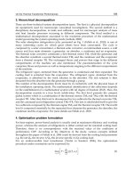
We then consider a large operating range by using a nonlinear control scheme that stabilizes
the pendulum angle at the pendant position (see Appendix 9.2 for more details about the
controller used in this case study). Using this controller, a large operating range is obtained
as seen in Fig. 7. The same observers (Observers 2 and 3) are used in parallel with this control
scheme, and the resulting estimation errors are compared in Fig. 8. The two observers are also
Small-gain Luenberger High-gain Luenberger Lipschitz
max
|e

1
| 3.6485 0.4323 0.1716
max
|e
2
| 1.5681 0.0925 0.1865
Table 1. Case study 1 - Estimation errors “e
1
” and “e
2
” in degrees
pure state feedback High-gain Luenberger Lipschitz
Percentage of overshoot 20.3613% 12.7440% 48.4863%
|steady state error | 2.5635 3.4424 3.7939
Table 2. Case study 1 - Tracking performance in degrees
compared in observer-based control, and the Luenberger observer fails in this case, causing
total system unstability. The Lipschitz observer, on the other hand, runs successfully and its
performance (compared to the pure state feedback control) is shown in Fig. 9. This case study
illustrates the importance of the Lipschitz observer in large operating regions, where the linear
observer normally fails.
0 5 10 15 20 25 30
−40
−20
0
20
40
60
80
100
120

140
160
time (sec)
motor angle (deg)
(a)
0 5 10 15 20 25 30
−100
0
100
200
300
400
500
600
700
time (sec)
pendulum angle (deg)
(b)
Fig. 7. Case Study 1 - (a) Motor Response, (b) Pendulum Response.
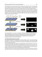
Finally, we conduct a comparison between static and dynamic Lipschitz observers, namely the
observer (6)-(7) and the one in (8)-(11). The comparison is between the new design proposed
in Section 3 and the one in Reference (Raghavan & Hedrick, 1994). First, the design algorithm
in (Raghavan & Hedrick, 1994) is tested for different values of α and ε. It fails for all values
of α
> 1, and the maximum attainable value is α = 1 (see L
5
in Appendix 9.2), while the
Lipschitz constant of the ROTPEN model is 44.45 as mentioned earlier. This observer is then
compared to the dynamic Lipschitz observer having the dynamic gain K
3

, and the estimation
errors are shown in Fig. 10. It is also important to note that the static Lipschitz observer fails
in stabilizing the system, when used in observer-based control, for both the small and large
operating range experiments. This shows the importance of the dynamic Lipschitz observer
design in this case.
MeasurementAnalysisandDiagnosisforRobot
ManipulatorsusingAdvancedNonlinearControlTechniques 155
mainly trigonometric terms, and using the symbolic MATLAB toolbox, an upper bound on
Φ(x, u) is found as 44.45, and hence the Lipschitz constant for the ROTPEN is α = 44.45.
This follows from the fact that if Φ :
n
× →
m
is continuously differentiable on a domain
D and the derivative of Φ with respect to the ﬁrst argument satisﬁes

∂Φ
∂x
 ≤ α on D, then Φ
is Lipschitz continuous on D with constant α, i.e.:
Φ(x, u) − Φ(y, u) ≤ α x − y, ∀ x, y ∈ D (42)
There are two encoders to measure the angle of the servomotor output shaft (θ
1
) and the angle
of the pendulum (θ
2
). An encoder is also available to measure the motor velocity
˙
θ
1

, but
no one is available to measure the pendulum velocity
˙
θ
2
. In the experiments, linear as well as
nonlinear control schemes are used to stabilize the pendulum at the inverted position (θ
2
= 0),
while tracking a step input of 30 degrees for the motor angle.
6.2 Case Study 1 - Lipschitz Observer Design
In this experiment, we focus on the nonlinear state estimation problem when no measure-
ment errors are affecting the system. We consider situations in which the operating range of
the pendulum is either close or far from the equilibrium point, comparing the Luenberger ob-
server with the Lipschitz observer in these cases. For the purpose of applying the Lipschitz
observer design, the nonlinear model discussed in section 6.1 is used. We also compare the
dynamic Lipschitz observer of section 3 with the static design method in Reference (Raghavan
& Hedrick, 1994). In this case study the full-order linear and Lipschitz models are used for
observer design, where the output is assumed as y
= [x
1
x
2
]
T
(all the observer parameters
that are used in this experiment can be found in Appendix 9.2).
First, a linear state feedback controller is used to stabilize the system in a small operating
range around the inverted position, and three observers are compared:
1) Observer 1: A linear Luenberger observer where the observer gain is obtained by plac-

ing the poles of
(A − LC) at {−24, −3.8, −4.8, −12.8} (see L
3−small
in Appendix
9.2).
2) Observer 2: A high gain Luenberger observer, which has the same form of Observer
1 but with the poles placed at
{−200, −70, −20 + 15i, −20 − 15i} (see L
3−large
in
Appendix 9.2).
3) Observer 3: A Lipschitz observer of the form (8)-(11), based on the full-order Lipschitz
model of the ROTPEN. The dynamic gain is computed using the design procedure in
section 3.1, for α
= 44.45 (see K
3
in Appendix 9.2).
The three observers run successfully with stable estimation errors. Table 1 shows the maxi-
mum estimation errors in this case. It can be seen that both the Luenberger observer (large
poles) and the Lipschitz observer achieve comparable performance, which is much better than
the Luenberger observer with small poles. The three observers are also tested in observer-
based control, and their tracking performance is compared in Table 2. We conclude that, due
to the small operating range considered in this case study, a high-gain Luenberger observer
achieves a good performance in terms of the state estimation errors and the tracking errors.
We then consider a large operating range by using a nonlinear control scheme that stabilizes
the pendulum angle at the pendant position (see Appendix 9.2 for more details about the
controller used in this case study). Using this controller, a large operating range is obtained
as seen in Fig. 7. The same observers (Observers 2 and 3) are used in parallel with this control
scheme, and the resulting estimation errors are compared in Fig. 8. The two observers are also
Small-gain Luenberger High-gain Luenberger Lipschitz

max |e
1
| 3.6485 0.4323 0.1716
max |e
2
| 1.5681 0.0925 0.1865
Table 1. Case study 1 - Estimation errors “e
1
” and “e
2
” in degrees
pure state feedback High-gain Luenberger Lipschitz
Percentage of overshoot 20.3613% 12.7440% 48.4863%
|steady state error | 2.5635 3.4424 3.7939
Table 2. Case study 1 - Tracking performance in degrees
compared in observer-based control, and the Luenberger observer fails in this case, causing
total system unstability. The Lipschitz observer, on the other hand, runs successfully and its
performance (compared to the pure state feedback control) is shown in Fig. 9. This case study
illustrates the importance of the Lipschitz observer in large operating regions, where the linear
observer normally fails.
0 5 10 15 20 25 30
−40
−20
0
20
40
60
80
100
120

e1
e2
Fig. 8. Case Study 1 - (a) High-gain Luenberger Errors, (b) Dynamic Lipschitz Errors.
0 5 10 15 20 25 30
−100
0
100
200
300
400
500
600
700
time (sec)
(deg)
(a)
state feedback
Lipschitz observer−based feedback
0 5 10 15 20 25 30
−100
−50
0
50
100
150
200
time (sec)
(deg)
(b)
state feedback

Lipschitz observer−based feedback
Fig. 9. Case Study 1 - (a) Pendulum Angle, (b) Motor Angle.
6.3 Case Study 2 - Lipschitz Measurement Error Diagnosis
In this experiment, the results of Sections 4 and 5 are assessed on the nonlinear Lipschitz
model. A large operating range is considered by using a nonlinear, switching, LQR control
scheme (with integrator) that stabilizes the pendulum at the inverted position (starting from
the pendant position) while tracking a step input of 30 degrees for the motor angle as seen in
Fig. 11 (the no-bias case). In the ﬁrst part of this experiment, an important measurement error
that affects the ROTPEN in real-time is considered. This is a sensor fault introduced by the
pendulum encoder. The encoder returns the pendulum angle relative to the initial condition,
assuming this initial condition to be θ
2
= 0. This constitutes a source of bias, as shown in
Fig. 11(b), when the pendulum initial condition is unknown or is deviated from the inverted
position. The effect of this measurement error on the tracking performance is also illustrated
in Fig. 11(a) for two different bias situations. The dynamic Lipschitz observer (discussed in
section 4) is applied to diagnose and tolerate this fault. In addition to this bias fault, the
observer is also applied for a 2 rad/sec fault introduced in real-time, as well as for the case of
a low frequency fault in the range
[0, 1 rad/sec].
0 5 10 15 20 25 30
−20
0
20
40
60
80
100
time (sec)
(deg)

(a)
dynamic Lipschitz observer
static Lipschitz observer
0 5 10 15 20 25 30
−250
−200
−150
−100
−50
0
50
100
(b)
time (sec)
(deg)
dynamic Lipschitz observer
static Lipschitz observer
Fig. 10. Case Study 1 - (a) Estimation Error “e
1
”, (b) Estimation Error “e
2
”.
0 5 10 15 20 25 30 35 40 45 50
−30
0
30
60
90
120
150

180
210
240
270
(a)
time (sec)
motor angle (deg)
No bias
Small bias
Large bias
0 5 10 15 20 25 30 35 40 45 50
−30
−20
−10
0
10
20
30
40
50
(b)
time (sec)
pendulum angle (deg)
No bias
Small bias
Large bias
bias= −8.965
bias= −13.623
Fig. 11. Case Study 2 - (a) Tracking Performance, (b) Pendulum Angle.
First, the design procedure in section 4 is used to accurately estimate and tolerate the bias

faults shown in Fig. 11(b). This is the special case where ω
o
= 0. Using the reduced-order
Lipschitz model with α
= 44.45 (and using the LMI design procedure, the dynamic gain for
the observer (8)-(12) that achieves measurement error identiﬁcation is obtained as K
6
(see Ap-
pendix 9.3 for more details). Using this observer, the biases affecting the system in Fig. 11 are
successfully estimated as shown in Fig. 12. Moreover, by using this observer in an observer-
based control scheme, the tracking performance in the large bias case is illustrated in Fig. 13.
The performance is much improved over the one with no fault tolerance as seen in Fig. 13(b).
It also gives less overshoot than the no bias case, as seen in Fig. 13(a). Similar results are
obtained for the small bias case.
The case of measurement error in the form of harmonics is now considered, with a sensor
fault having a frequency of 2 rad/sec. The dynamic gain for the observer (8)-(12) is computed
using the design approach discussed in section 5. This is the special case where ω
o
= 2. The
gain is obtained at λ
= 10
−12
as K
7
(see Appendix 9.3). Using this observer, Fig. 14 shows the
correct estimation of a measurement error of amplitude 20 degrees and frequency 2 rad/sec.
MeasurementAnalysisandDiagnosisforRobot
ManipulatorsusingAdvancedNonlinearControlTechniques 157
0 5 10 15 20 25 30
−10

−5
0
5
10
15
20
time (sec)
(deg)
(a)
e1
e2
0 5 10 15 20 25
−10
−5
0
5
10
15
20
time (sec)
(deg)
(b)
e1
e2
Fig. 8. Case Study 1 - (a) High-gain Luenberger Errors, (b) Dynamic Lipschitz Errors.
0 5 10 15 20 25 30
−100
0
100
200

300
400
500
600
700
time (sec)
(deg)
(a)
state feedback
Lipschitz observer−based feedback
0 5 10 15 20 25 30
−100
−50
0
50
100
150
200
time (sec)
(deg)
(b)
state feedback
Lipschitz observer−based feedback
Fig. 9. Case Study 1 - (a) Pendulum Angle, (b) Motor Angle.
6.3 Case Study 2 - Lipschitz Measurement Error Diagnosis
In this experiment, the results of Sections 4 and 5 are assessed on the nonlinear Lipschitz
model. A large operating range is considered by using a nonlinear, switching, LQR control
scheme (with integrator) that stabilizes the pendulum at the inverted position (starting from
the pendant position) while tracking a step input of 30 degrees for the motor angle as seen in
Fig. 11 (the no-bias case). In the ﬁrst part of this experiment, an important measurement error

that affects the ROTPEN in real-time is considered. This is a sensor fault introduced by the
pendulum encoder. The encoder returns the pendulum angle relative to the initial condition,
assuming this initial condition to be θ
2
= 0. This constitutes a source of bias, as shown in
Fig. 11(b), when the pendulum initial condition is unknown or is deviated from the inverted
position. The effect of this measurement error on the tracking performance is also illustrated
in Fig. 11(a) for two different bias situations. The dynamic Lipschitz observer (discussed in
section 4) is applied to diagnose and tolerate this fault. In addition to this bias fault, the
observer is also applied for a 2 rad/sec fault introduced in real-time, as well as for the case of
a low frequency fault in the range
[0, 1 rad/sec].
0 5 10 15 20 25 30
−20
0
20
40
60
80
100
time (sec)
(deg)
(a)
dynamic Lipschitz observer
static Lipschitz observer
0 5 10 15 20 25 30
−250
−200
−150
−100

−50
0
50
100
(b)
time (sec)
(deg)
dynamic Lipschitz observer
static Lipschitz observer
Fig. 10. Case Study 1 - (a) Estimation Error “e
1
”, (b) Estimation Error “e
2
”.
0 5 10 15 20 25 30 35 40 45 50
−30
0
30
60
90
120
150
180
210
240
270
(a)
time (sec)
motor angle (deg)
No bias

Small bias
Large bias
0 5 10 15 20 25 30 35 40 45 50
−30
−20
−10
0
10
20
30
40
50
(b)
time (sec)
pendulum angle (deg)
No bias
Small bias
Large bias
bias= −8.965
bias= −13.623
Fig. 11. Case Study 2 - (a) Tracking Performance, (b) Pendulum Angle.
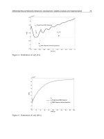
First, the design procedure in section 4 is used to accurately estimate and tolerate the bias
faults shown in Fig. 11(b). This is the special case where ω
o
= 0. Using the reduced-order
Lipschitz model with α
= 44.45 (and using the LMI design procedure, the dynamic gain for
the observer (8)-(12) that achieves measurement error identiﬁcation is obtained as K
6
(see Ap-

pendix 9.3 for more details). Using this observer, the biases affecting the system in Fig. 11 are
successfully estimated as shown in Fig. 12. Moreover, by using this observer in an observer-
based control scheme, the tracking performance in the large bias case is illustrated in Fig. 13.
The performance is much improved over the one with no fault tolerance as seen in Fig. 13(b).
It also gives less overshoot than the no bias case, as seen in Fig. 13(a). Similar results are
obtained for the small bias case.
The case of measurement error in the form of harmonics is now considered, with a sensor
fault having a frequency of 2 rad/sec. The dynamic gain for the observer (8)-(12) is computed
using the design approach discussed in section 5. This is the special case where ω
o
= 2. The
gain is obtained at λ
= 10
−12
as K
7
(see Appendix 9.3). Using this observer, Fig. 14 shows the
correct estimation of a measurement error of amplitude 20 degrees and frequency 2 rad/sec.
RobotManipulators,TrendsandDevelopment158
5 10 15 20 25 30 35 40 45 50
−100
−50
0
50
100
150
(a)
time (sec)
(deg)
Residual

Actual bias
0 5 10 15 20 25 30 35 40 45 50
−100
−80
−60
−40
−20
0
20
40
60
80
100
(b)
time (sec)
(deg)
Residual
Actual bias
Fig. 12. Case Study 2 - (a) Estimation of the Small Bias, (b) Estimation of the Large Bias.
0 5 10 15 20 25 30 35 40 45 50
−50
0
30
60
90
time (sec)
motor angle (deg)
(a)
No bias response
Large bias with observer−based control

0 5 10 15 20 25 30 35 40 45 50
−50
0
50
100
150
200
250
300
(b)
time (sec)
motor angle (deg)
Large bias response
Large bias with observer−based control
Fig. 13. Case Study 2 - (a) No-bias versus Observer-based, (b) Large Bias versus Observer-
based.
We then consider the case of low frequency sensor faults (in the range
[0, 1 rad/sec]). Using
the design introduced in section 5 (and with a
= 0.1, b = 1 and  = 0.1), the optimal observer
gain is obtained using the command hinﬂmi in MATLAB, with minimum λ as 10
−12
(see K
8
in Appendix 9.3). Using this observer for measurement error diagnosis, a correct estimation
of a low frequency sensor fault (generated using the MATLAB command idinput) is shown in
Fig. 15.
7. Conclusion
The Lipschitz observer design approach provides an important framework for solving the
measurement error diagnosis problem in robot manipulators. The classical observer structure

is not directly applicable to the detection and identiﬁcation problems. This is in part due to the
restrictive observer structure, and also due to the idealized assumptions inherent in this struc-
ture that do not take into account uncertain model parameters and disturbances. The dynamic
observer structure offers two important advantages in that regard: (i) The observer stability
condition that ensures asymptotic convergence of the state estimates is satisﬁed by a family
0 5 10 15 20 25 30 35 40 45 50
−50
−40
−30
−20
−10
0
10
20
30
40
50
time (sec)
(deg)
actual fault
residual
Fig. 14. Case Study 2 - Frequency Band Estimation.
0 10 20 30 40 50 60 70 80 90 100
−50
−40
−30
−20
−10
0
10

20
30
40
50
time (sec)
(deg)
Actual fault
Residual
Fig. 15. Case Study 2 - Diagnosis of Low Frequency Sensor Fault.
of observers, adding extra degrees of freedom to the observer which lay the ground to the ad-
dition of the detection and identiﬁcation objectives in the design, (ii) The observer design can
be carried out using a systematic design procedure which is less restrictive than the existing
design approaches and which is solvable using commercially available software. The design
depends heavily on the nature of the objectives considered. While an analytical solution can
be used for measurement error detection, the identiﬁcation problem is more demanding and
needs a more general design framework. This problem is shown to be equivalent to a standard
convex optimization problem which is solvable using Linear Matrix Inequalities (LMIs). Us-
ing this generalized framework, different frequency patterns for the measurement errors that
affect the robot manipulator could be considered, and systematic design procedures could be
used to solve the problem. A practical example, namely the Quanser rotary inverted pendu-
lum (ROTPEN) in the Control Systems Lab, Electrical and Computer Engineering department,
University of Alberta, is used to illustrate these results. The ROTPEN model falls in the cate-
gory of planar robot manipulators, and the experimental results illustrate the applicability of
the proposed techniques in the robotics ﬁeld by showing the following:
MeasurementAnalysisandDiagnosisforRobot
ManipulatorsusingAdvancedNonlinearControlTechniques 159
5 10 15 20 25 30 35 40 45 50
−100
−50
0

50
100
150
(a)
time (sec)
(deg)
Residual
Actual bias
0 5 10 15 20 25 30 35 40 45 50
−100
−80
−60
−40
−20
0
20
40
60
80
100
(b)
time (sec)
(deg)
Residual
Actual bias
Fig. 12. Case Study 2 - (a) Estimation of the Small Bias, (b) Estimation of the Large Bias.
0 5 10 15 20 25 30 35 40 45 50
−50
0
30

60
90
time (sec)
motor angle (deg)
(a)
No bias response
Large bias with observer−based control
0 5 10 15 20 25 30 35 40 45 50
−50
0
50
100
150
200
250
300
(b)
time (sec)
motor angle (deg)
Large bias response
Large bias with observer−based control
Fig. 13. Case Study 2 - (a) No-bias versus Observer-based, (b) Large Bias versus Observer-
based.
We then consider the case of low frequency sensor faults (in the range
[0, 1 rad/sec]). Using
the design introduced in section 5 (and with a
= 0.1, b = 1 and  = 0.1), the optimal observer
gain is obtained using the command hinﬂmi in MATLAB, with minimum λ as 10
−12
(see K

8
in Appendix 9.3). Using this observer for measurement error diagnosis, a correct estimation
of a low frequency sensor fault (generated using the MATLAB command idinput) is shown in
Fig. 15.
7. Conclusion
The Lipschitz observer design approach provides an important framework for solving the
measurement error diagnosis problem in robot manipulators. The classical observer structure
is not directly applicable to the detection and identiﬁcation problems. This is in part due to the
restrictive observer structure, and also due to the idealized assumptions inherent in this struc-
ture that do not take into account uncertain model parameters and disturbances. The dynamic
observer structure offers two important advantages in that regard: (i) The observer stability
condition that ensures asymptotic convergence of the state estimates is satisﬁed by a family
0 5 10 15 20 25 30 35 40 45 50
−50
−40
−30
−20
−10
0
10
20
30
40
50
time (sec)
(deg)
actual fault
residual
Fig. 14. Case Study 2 - Frequency Band Estimation.
0 10 20 30 40 50 60 70 80 90 100

−50
−40
−30
−20
−10
0
10
20
30
40
50
time (sec)
(deg)
Actual fault
Residual
Fig. 15. Case Study 2 - Diagnosis of Low Frequency Sensor Fault.
of observers, adding extra degrees of freedom to the observer which lay the ground to the ad-
dition of the detection and identiﬁcation objectives in the design, (ii) The observer design can
be carried out using a systematic design procedure which is less restrictive than the existing
design approaches and which is solvable using commercially available software. The design
depends heavily on the nature of the objectives considered. While an analytical solution can
be used for measurement error detection, the identiﬁcation problem is more demanding and
needs a more general design framework. This problem is shown to be equivalent to a standard
convex optimization problem which is solvable using Linear Matrix Inequalities (LMIs). Us-
ing this generalized framework, different frequency patterns for the measurement errors that
affect the robot manipulator could be considered, and systematic design procedures could be
used to solve the problem. A practical example, namely the Quanser rotary inverted pendu-
lum (ROTPEN) in the Control Systems Lab, Electrical and Computer Engineering department,
University of Alberta, is used to illustrate these results. The ROTPEN model falls in the cate-
gory of planar robot manipulators, and the experimental results illustrate the applicability of

the proposed techniques in the robotics ﬁeld by showing the following:
RobotManipulators,TrendsandDevelopment160
i) How to model a robot manipulator as a standard Lipschitz system.
ii) The importance of the dynamic Lipschitz observer in large operating regions where the
linear observer normally fails.
iii) The accurate velocity estimations obtained using the dynamic observer, alleviating the
need to introduce velocity sensors in real-time.
iv) How the static observer fails, compared to the dynamic observer, when applied to
Robotic Systems due to the large Lipschitz constant that these systems normally have.
v) The efﬁciency of the dynamic observer in diagnosing and tolerating measurement er-
rors of different frequencies, including an important bias introduced by the error in the
initial conditions of the pendulum encoder.
8. Acknowledgement
The author would like to thank the Advanced Control Systems Laboratory members at Uni-
versity of Alberta. Special thanks to Dr. Alan Lynch and to Dr. Thomas Grochmal for pro-
viding the ROTPEN equations and the switching swingup control scheme used in the experi-
ments.
9. Appendix
9.1 The ROTPEN Model
The system parameters are: l
1
= 0.215 m, l
2
= 0.335 m, m
2
= 0.1246 Kg, β = 0.135Nm/s,
µ
= 0.2065Nm/V, b
2
= 0.0018Kg/s, g = 9.81m/s

2
, and J
1
= 0.0064 Kg.m
2
. With the state
deﬁned as x
= [x
1
x
2
x
3
x
4
]
T
= [θ
1
(rad) θ
2
(rad)
˙
θ
1
(rad/s)
˙
θ
2
(rad/s)]

T
, the state space model
has the form
˙
x
= f(x ) + g (x)u as follows (This model was derived in Lynch (2004)):
˙
x
=





x
3
x
4
h
3
(x) −
m
2
l
2
2
βx
3
3∆
h

4
(x) +
m
2
l
1
l
2
βc
2
2∆





+





0
0
µm
2
l
2
2
3∆

−µm
2
l
1
l
2
c
2
2∆





u
where s
k
= sin(x
k
), c
k
= cos(x
k
) are used to simplify notation, and where:
h
3
(x) =
m
2
2

l
2
2

−
1
2
gl
1
s
2
c
2
−
1
4
l
1
l
2
x
2
3
s
2
c
2
2
+ b
2

l
1
x
4
c
2
/(m
2
l
2
) +
1
3
l
1
l
2
x
2
4
s
2
−
1
3
l
2
2
x
3

x
4
s
2
c
2

2∆
h
4
(x) =
1
2
m
2
gl
2

m
2
l
2
1
+
1
4
m
2
l
2

2
s
2
2
+ J
1

s
2
∆
−

m
2
l
2
1
+
1
4
m
2
l
2
2
s
2
2
+ J
1


b
2
x
4
∆
+
1
4
m
2
l
2
2
[m
2
l
2
1
(x
2
3
− x
2
4
)s
2
c
2
+

1
4
m
2
l
2
2
x
2
3
s
3
2
c
2
+ J
1
x
2
3
s
2
c
2
+ m
2
l
1
l
2

x
3
x
4
s
2
c
2
2
]
∆
∆
= m
2
l
2
2

1
3
m
2
l
2
1
+
1
12
m
2

l
2
2
s
2
2
+
1
3
J
1
−
1
4
m
2
l
2
1
c
2
2

.
9.2 Models and Parameters for Case Study 1
Luenberger observer with small gain :
L
3−small
=


5.9207
−7.4414 −13.0209 −9.9019
−1.5356 21.6603 −7.2493 108.1343

T
.
High-gain Luenberger observer
:
L
3−large
= 10
3

0.0716 0.0070 0.1432
−0.5022
0.0203 0.2206 1.4312 4.4841

T
.
Dynamic Lipschitz observer : (K
3
, obtained for α = 44.45,  = β = 0.00048828)
A
L3
=10
4





−0.3428 0 0 0
0
−0.3428 0 0
−6.2073 0 −0.2048 0
0
−6.2073 0 −0.2048




, B
L3
= 10
4




0.138 0
0 0.138
6.2072 0
0 6.2072




,
C
L3
=10

3




2.048 0 0.0005 0
0 2.048 0 0.0005
0.0005 0 2.0480
0 0.0005 0 2.0485




, D
L3
=




0 0
0 0
0 0
0 0




.
Nonlinear “normal form” Controller

:
By considering y
= x
2
, and using the nonlinear model of the ROTPEN in Appendix 9.1, the
following coordinate transformation:




ξ
1
ξ
2
η
1
η
2




=





x
2

x
4
x
1
x
3

l
1
2
c
2

+ x
4
l
2
3





is used to put the system in the so-called normal or tracking form (Marino & Tomei, 1995), that
is:




˙

ξ
1
˙
ξ
2
˙
η
1
˙
η
2




=




ξ
2
f
4
(x) + g
4
(x)u
x
3
−

l
1
2
x
3
x
4
s
2
+
l
1
2
c
2
f
3
(x) +
l
2
3
f
4
(x)




and using the control law:
u

=
1
g
4
(x)
[
−
9x
2
− 6x
4
− f
4
(x)
]
where f
4
(x) and g
4
(x) denote the 4
th
elements of f (x) and g(x) in Appendix 9.1 respectively.
The subsystem
(
ξ
1
, ξ
2
)
is then stabilized. It is important to note that the zero dynamics in this

case, i.e the subsystem
(
η
1
, η
2
)
is unstable, and therefore the motor angle is not guaranteed to
converge to the reference input.
Static Lipschitz observer : (obtained for α = 1, ε = 0.5)
L
5
=

1.7108
−2.1247 1.9837 −5.4019
0.4338
−0.2089 1.1030 −2.8972

T
.
MeasurementAnalysisandDiagnosisforRobot
ManipulatorsusingAdvancedNonlinearControlTechniques 161
i) How to model a robot manipulator as a standard Lipschitz system.
ii) The importance of the dynamic Lipschitz observer in large operating regions where the
linear observer normally fails.
iii) The accurate velocity estimations obtained using the dynamic observer, alleviating the
need to introduce velocity sensors in real-time.
iv) How the static observer fails, compared to the dynamic observer, when applied to
Robotic Systems due to the large Lipschitz constant that these systems normally have.

v) The efﬁciency of the dynamic observer in diagnosing and tolerating measurement er-
rors of different frequencies, including an important bias introduced by the error in the
initial conditions of the pendulum encoder.
8. Acknowledgement
The author would like to thank the Advanced Control Systems Laboratory members at Uni-
versity of Alberta. Special thanks to Dr. Alan Lynch and to Dr. Thomas Grochmal for pro-
viding the ROTPEN equations and the switching swingup control scheme used in the experi-
ments.
9. Appendix
9.1 The ROTPEN Model
The system parameters are: l
1
= 0.215 m, l
2
= 0.335 m, m
2
= 0.1246 Kg, β = 0.135Nm/s,
µ
= 0.2065Nm/V, b
2
= 0.0018Kg/s, g = 9.81m/s
2
, and J
1
= 0.0064 Kg.m
2
. With the state
deﬁned as x
= [x
1

x
2
x
3
x
4
]
T
= [θ
1
(rad) θ
2
(rad)
˙
θ
1
(rad/s)
˙
θ
2
(rad/s)]
T
, the state space model
has the form
˙
x
= f(x ) + g (x)u as follows (This model was derived in Lynch (2004)):
˙
x
=






x
3
x
4
h
3
(x) −
m
2
l
2
2
βx
3
3∆
h
4
(x) +
m
2
l
1
l
2
βc

2
2∆





+





0
0
µm
2
l
2
2
3∆
−µm
2
l
1
l
2
c
2
2∆






u
where s
k
= sin(x
k
), c
k
= cos(x
k
) are used to simplify notation, and where:
h
3
(x) =
m
2
2
l
2
2

−
1
2
gl
1

s
2
c
2
−
1
4
l
1
l
2
x
2
3
s
2
c
2
2
+ b
2
l
1
x
4
c
2
/(m
2
l

2
) +
1
3
l
1
l
2
x
2
4
s
2
−
1
3
l
2
2
x
3
x
4
s
2
c
2

2∆
h

4
(x) =
1
2
m
2
gl
2

m
2
l
2
1
+
1
4
m
2
l
2
2
s
2
2
+ J
1

s
2

∆
−

m
2
l
2
1
+
1
4
m
2
l
2
2
s
2
2
+ J
1

b
2
x
4
∆
+
1
4

m
2
l
2
2
[m
2
l
2
1
(x
2
3
− x
2
4
)s
2
c
2
+
1
4
m
2
l
2
2
x
2

3
s
3
2
c
2
+ J
1
x
2
3
s
2
c
2
+ m
2
l
1
l
2
x
3
x
4
s
2
c
2
2

]
∆
∆
= m
2
l
2
2

1
3
m
2
l
2
1
+
1
12
m
2
l
2
2
s
2
2
+
1
3

J
1
−
1
4
m
2
l
2
1
c
2
2

.
9.2 Models and Parameters for Case Study 1
Luenberger observer with small gain :
L
3−small
=

5.9207
−7.4414 −13.0209 −9.9019
−1.5356 21.6603 −7.2493 108.1343

T
.
High-gain Luenberger observer
:
L

3−large
= 10
3

0.0716 0.0070 0.1432
−0.5022
0.0203 0.2206 1.4312 4.4841

T
.
Dynamic Lipschitz observer : (K
3
, obtained for α = 44.45,  = β = 0.00048828)
A
L3
=10
4




−0.3428 0 0 0
0
−0.3428 0 0
−6.2073 0 −0.2048 0
0
−6.2073 0 −0.2048





, B
L3
= 10
4




0.138 0
0 0.138
6.2072 0
0 6.2072




,
C
L3
=10
3




2.048 0 0.0005 0
0 2.048 0 0.0005
0.0005 0 2.0480
0 0.0005 0 2.0485





, D
L3
=




0 0
0 0
0 0
0 0




.
Nonlinear “normal form” Controller
:
By considering y
= x
2
, and using the nonlinear model of the ROTPEN in Appendix 9.1, the
following coordinate transformation:





ξ
1
ξ
2
η
1
η
2




=





x
2
x
4
x
1
x
3

l
1

2
c
2

+ x
4
l
2
3





is used to put the system in the so-called normal or tracking form (Marino & Tomei, 1995), that
is:




˙
ξ
1
˙
ξ
2
˙
η
1
˙

η
2




=




ξ
2
f
4
(x) + g
4
(x)u
x
3
−
l
1
2
x
3
x
4
s
2

+
l
1
2
c
2
f
3
(x) +
l
2
3
f
4
(x)




and using the control law:
u
=
1
g
4
(x)
[
−
9x
2

− 6x
4
− f
4
(x)
]
where f
4
(x) and g
4
(x) denote the 4
th
elements of f (x) and g(x) in Appendix 9.1 respectively.
The subsystem
(
ξ
1
, ξ
2
)
is then stabilized. It is important to note that the zero dynamics in this
case, i.e the subsystem
(
η
1
, η
2
)
is unstable, and therefore the motor angle is not guaranteed to
converge to the reference input.

Static Lipschitz observer : (obtained for α = 1, ε = 0.5)
L
5
=

1.7108
−2.1247 1.9837 −5.4019
0.4338
−0.2089 1.1030 −2.8972

T
.
RobotManipulators,TrendsandDevelopment162
9.3 Models and Parameters for Case Study 2
Lipschitz reduced-order model for observer design (
¯
x = [θ
2
˙
θ
1
˙
θ
2
]
T
) :
˙
¯
x

=


0 0 1
−25.14 −17.22 0.2210
68.13 16.57
−0.599


¯
x
+


0
φ
1
(
¯
x, u
)
φ
2
(
¯
x, u
)


¯

y
=

1 0 0

¯
x
Lipschitz dynamic observer for sensor bias
: (K
6
, obtained for λ = 10
−12
,  = 0.1)
A
L6
=




−175.7353 3.8503 0.1710 −30.6336
16.8182
−171.9539 26.7652 32.1257
35.1361 16.5360
−97.3465 114.1349
−87.9041 25.7568 62.1442 −87.8099





, B
L6
=




5.0462
−44.8932
−75.4539
106.5497




,
C
L6
=


167.6750
−5.0531 −8.5208 42.0138
−7.1899 155.5373 −42.6804 −11.1441
5.3053
−18.7128 −120.8293 171.1055


, D
L6

=


0
0
0


.
Lipschitz dynamic observer for fault of 2 rad/sec
: (K
7
, obtained for λ = 10
−12
,  = 0.1)
A
L7
=






−816.9997 −12.5050 −51.0842 −64.0861 31.8003
23.8482
−772.7024 149.1621 122.7602 −75.3718
−3.0714 139.9543 −412.1421 361.2027 −176.7926
−193.3011 128.2831 346.2370 −405.3024 201.2094
71.5547

−47.7237 −104.0209 129.8922 −64.7247






, B
L7
=






9.2096
−73.6540
−80.3861
177.6628
−67.4227






,
C
L7

=


809.4037 11.3091 28.1928 88.3295
−43.7581
−13.1309 758.2718 −276.6110 4.7255 12.0717
−15.9908 −176.8554 −509.7118 587.8999 −294.7496


, D
L7
=


0
0
0


.
Lipschitz dynamic observer for low frequencies : (K
8
, obtained for λ = 10
−12
,  = 0.1)
A
L8
=





−217.7814 1.8898 −4.8573 −38.2385
−1.5288 −185.0261 38.1186 36.8585
108.5437 28.4810
−87.0920 135.1710
−618.9648 28.9348 82.1016 −164.6086




, B
L8
=




−30.2950
26.3896
147.7784
−637.5223




,
C
L8
=



−184.6168 3.4213 1.8716 −51.2266
6.5728
−171.5615 49.1851 16.3542
−4.3022 15.0586 114.2413 −224.5769


, D
L8
=


0
0
0


.
10. References
Aboky, C., Sallet, G. & Vivalda, J. (2002). Observers for Lipschitz nonlinear systems, Int. J. of
Contr., vol. 75, No. 3, pp. 204-212.
Adjallah, K., Maquin, D. & Ragot, J. (1994). Nonlinear observer based fault detection, IEEE
Trans. on Automat. Contr., pp. 1115-1120.
Chen, R., Mingori, D. & Speyer, J. (2003). Optimal stochastic fault detection ﬁlter, Automatica,
vol. 39, No. 3, pp. 377-390.
Chen, J. & Patton, R. (1999). Robust model-based fault diagnosis for dynamic systems, Kluwer Aca-
demic Publishers.
Doyle, J., Glover, K., Khargonekar P. & Francis, B. (1989). State spce solutions to standard H
2

and H
∞
control problems, IEEE Trans. Automat. Contr., Vol. 34, No. 8, pp. 831-847.
Frank, P. (1990). Fault diagnosis in dynamic systems using analytical and knowledge-based
redundancy - A survey and some new results, Automatica, vol. 26, No. 3, pp. 459-474.
Gahinet, P. & Apkarian, P. (1994). A linear matrix inequality approach to H
∞
control, Int. J. of
Robust and Nonlinear Contr., vol. 4, pp. 421-448.
Garcia, E. & Frank, P. (1997). Deterministic nonlinear observer based approaches to fault di-
agnosis: A survey, Contr. Eng. Practice, vol. 5, No. 5, pp. 663-670.
Hammouri, H., Kinnaert, M. & El Yaagoubi, E. (1999). Observer-based approach to fault de-
tection and isolation for nonlinear systems, IEEE Trans. on Automat. Contr., vol. 44,
No. 10.
Hill, D. & Moylan, P. (1977). Stability Results for Nonlinear Feedback Systems, Automatica,
Vol. 13, pp. 377-382.
Iwasaki, T. & Skelton, R. (1994). All controllers for the general H
∞
control problem: LMI exis-
tence conditions and state space formulas, Automatica, Vol. 30, No. 8, pp. 1307-1317.
Kabore, P. & Wang, H. (2001). Design of fault diagnosis ﬁlters and fault-tolerant control for a
class of nonlinear systems, IEEE Trans. on Automat. Contr., vol. 46, No. 11.
Lynch, A. (2004). Control Systems II (Lab Manual), University of Alberta.
Marino, R. & Tomei, P. (1995). Nonlinear Control Design - Geometric, Adaptive and Robust, Pren-
tice Hall Europe, 1995.
Marquez, H. (2003). Nonlinear Control Systems: Analysis and Design, Wiley, NY.
Pertew, A. (2006). Nonlinear observer-based fault detection and diagnosis, Ph.D Thesis, De-
partment of Electrical and Computer Engineering, University of Alberta.
Pertew, A., Marquez, H. & Zhao, Q. (2005). H
∞

synthesis of unknown input observers for
nonlinear Lipschitz systems, International J. Contr., vol. 78, No. 15, pp. 1155-1165.
Pertew, A., Marquez, H. & Zhao, Q. (2006). H
∞
observer design for Lipschitz nonlinear sys-
tems, IEEE Trans. on Automat. Contr., vol. 51, No. 7, pp. 1211-1216.
Pertew, A., Marquez, H. & Zhao, Q. (2007). LMI-based sensor fault diagnosis for nonlinear
Lipschitz systems, IEEE Trans. on Automat. Contr., vol. 43, pp. 1464-1469.
Raghavan, S. & Hedrick, J. (1994). Observer design for a class of nonlinear systems, Int. J. of
Contr., vol. 59, No. 2, pp. 5515-528.
Rajamani, R. (1998). Observers for Lipschitz nonlinear systems, IEEE Trans. on Automat. Contr.,
vol. 43, No. 3, pp. 397-401.
Rajamani, R. & Cho, Y. (1998). Existence and design of observers for nonlinear systems: rela-
tion to distance of unobservability, Int. J. Contr., Vol. 69, pp. 717-731.
Scherer, C. (1992). H
∞
optimization without assumptions on ﬁnite or inﬁnite zeros, Int. J. Contr.
and Optim., Vol. 30, No. 1, pp. 143-166.
Sciavicco, L. & Sicliano, B. (1989). Modeling and Control of Robot Manipulators, McGraw Hill.
Stoorvogel, A. (1996). The H
∞
control problem with zeros on the boundary of the stability
domain, Int. J. Contr., Vol. 63, pp. 1029-1053.
Vemuri, A. (2001). Sensor bias fault diagnosis in a class of nonlinear systems, IEEE Trans. on
Automat. Contr., vol. 46, No. 6.
Wang, H., Huang, Z. & Daley, S. (1997). On the Use of Adaptive Updating Rules for Actuator
and Sensor Fault Diagnosis, Automatica, Vol. 33, No. 2, pp. 217-225.
MeasurementAnalysisandDiagnosisforRobot
ManipulatorsusingAdvancedNonlinearControlTechniques 163
9.3 Models and Parameters for Case Study 2

Lipschitz reduced-order model for observer design (
¯
x = [θ
2
˙
θ
1
˙
θ
2
]
T
) :
˙
¯
x
=


0 0 1
−25.14 −17.22 0.2210
68.13 16.57
−0.599


¯
x
+



0
φ
1
(
¯
x, u
)
φ
2
(
¯
x, u
)


¯
y
=

1 0 0

¯
x
Lipschitz dynamic observer for sensor bias
: (K
6
, obtained for λ = 10
−12
,  = 0.1)
A

L6
=




−175.7353 3.8503 0.1710 −30.6336
16.8182
−171.9539 26.7652 32.1257
35.1361 16.5360
−97.3465 114.1349
−87.9041 25.7568 62.1442 −87.8099




, B
L6
=




5.0462
−44.8932
−75.4539
106.5497





,
C
L6
=


167.6750
−5.0531 −8.5208 42.0138
−7.1899 155.5373 −42.6804 −11.1441
5.3053
−18.7128 −120.8293 171.1055


, D
L6
=


0
0
0


.
Lipschitz dynamic observer for fault of 2 rad/sec
: (K
7
, obtained for λ = 10
−12

,  = 0.1)
A
L7
=






−816.9997 −12.5050 −51.0842 −64.0861 31.8003
23.8482
−772.7024 149.1621 122.7602 −75.3718
−3.0714 139.9543 −412.1421 361.2027 −176.7926
−193.3011 128.2831 346.2370 −405.3024 201.2094
71.5547
−47.7237 −104.0209 129.8922 −64.7247






, B
L7
=







9.2096
−73.6540
−80.3861
177.6628
−67.4227






,
C
L7
=


809.4037 11.3091 28.1928 88.3295
−43.7581
−13.1309 758.2718 −276.6110 4.7255 12.0717
−15.9908 −176.8554 −509.7118 587.8999 −294.7496


, D
L7
=



0
0
0


.
Lipschitz dynamic observer for low frequencies : (K
8
, obtained for λ = 10
−12
,  = 0.1)
A
L8
=




−217.7814 1.8898 −4.8573 −38.2385
−1.5288 −185.0261 38.1186 36.8585
108.5437 28.4810
−87.0920 135.1710
−618.9648 28.9348 82.1016 −164.6086




, B
L8
=





−30.2950
26.3896
147.7784
−637.5223




,
C
L8
=


−184.6168 3.4213 1.8716 −51.2266
6.5728
−171.5615 49.1851 16.3542
−4.3022 15.0586 114.2413 −224.5769


, D
L8
=


0

0
0


.
10. References
Aboky, C., Sallet, G. & Vivalda, J. (2002). Observers for Lipschitz nonlinear systems, Int. J. of
Contr., vol. 75, No. 3, pp. 204-212.
Adjallah, K., Maquin, D. & Ragot, J. (1994). Nonlinear observer based fault detection, IEEE
Trans. on Automat. Contr., pp. 1115-1120.
Chen, R., Mingori, D. & Speyer, J. (2003). Optimal stochastic fault detection ﬁlter, Automatica,
vol. 39, No. 3, pp. 377-390.
Chen, J. & Patton, R. (1999). Robust model-based fault diagnosis for dynamic systems, Kluwer Aca-
demic Publishers.
Doyle, J., Glover, K., Khargonekar P. & Francis, B. (1989). State spce solutions to standard H
2
and H
∞
control problems, IEEE Trans. Automat. Contr., Vol. 34, No. 8, pp. 831-847.
Frank, P. (1990). Fault diagnosis in dynamic systems using analytical and knowledge-based
redundancy - A survey and some new results, Automatica, vol. 26, No. 3, pp. 459-474.
Gahinet, P. & Apkarian, P. (1994). A linear matrix inequality approach to H
∞
control, Int. J. of
Robust and Nonlinear Contr., vol. 4, pp. 421-448.
Garcia, E. & Frank, P. (1997). Deterministic nonlinear observer based approaches to fault di-
agnosis: A survey, Contr. Eng. Practice, vol. 5, No. 5, pp. 663-670.
Hammouri, H., Kinnaert, M. & El Yaagoubi, E. (1999). Observer-based approach to fault de-
tection and isolation for nonlinear systems, IEEE Trans. on Automat. Contr., vol. 44,
No. 10.

Hill, D. & Moylan, P. (1977). Stability Results for Nonlinear Feedback Systems, Automatica,
Vol. 13, pp. 377-382.
Iwasaki, T. & Skelton, R. (1994). All controllers for the general H
∞
control problem: LMI exis-
tence conditions and state space formulas, Automatica, Vol. 30, No. 8, pp. 1307-1317.
Kabore, P. & Wang, H. (2001). Design of fault diagnosis ﬁlters and fault-tolerant control for a
class of nonlinear systems, IEEE Trans. on Automat. Contr., vol. 46, No. 11.
Lynch, A. (2004). Control Systems II (Lab Manual), University of Alberta.
Marino, R. & Tomei, P. (1995). Nonlinear Control Design - Geometric, Adaptive and Robust, Pren-
tice Hall Europe, 1995.
Marquez, H. (2003). Nonlinear Control Systems: Analysis and Design, Wiley, NY.
Pertew, A. (2006). Nonlinear observer-based fault detection and diagnosis, Ph.D Thesis, De-
partment of Electrical and Computer Engineering, University of Alberta.
Pertew, A., Marquez, H. & Zhao, Q. (2005). H
∞
synthesis of unknown input observers for
nonlinear Lipschitz systems, International J. Contr., vol. 78, No. 15, pp. 1155-1165.
Pertew, A., Marquez, H. & Zhao, Q. (2006). H
∞
observer design for Lipschitz nonlinear sys-
tems, IEEE Trans. on Automat. Contr., vol. 51, No. 7, pp. 1211-1216.
Pertew, A., Marquez, H. & Zhao, Q. (2007). LMI-based sensor fault diagnosis for nonlinear
Lipschitz systems, IEEE Trans. on Automat. Contr., vol. 43, pp. 1464-1469.
Raghavan, S. & Hedrick, J. (1994). Observer design for a class of nonlinear systems, Int. J. of
Contr., vol. 59, No. 2, pp. 5515-528.
Rajamani, R. (1998). Observers for Lipschitz nonlinear systems, IEEE Trans. on Automat. Contr.,
vol. 43, No. 3, pp. 397-401.
Rajamani, R. & Cho, Y. (1998). Existence and design of observers for nonlinear systems: rela-
tion to distance of unobservability, Int. J. Contr., Vol. 69, pp. 717-731.

Scherer, C. (1992). H
∞
optimization without assumptions on ﬁnite or inﬁnite zeros, Int. J. Contr.
and Optim., Vol. 30, No. 1, pp. 143-166.
Sciavicco, L. & Sicliano, B. (1989). Modeling and Control of Robot Manipulators, McGraw Hill.
Stoorvogel, A. (1996). The H
∞
control problem with zeros on the boundary of the stability
domain, Int. J. Contr., Vol. 63, pp. 1029-1053.
Vemuri, A. (2001). Sensor bias fault diagnosis in a class of nonlinear systems, IEEE Trans. on
Automat. Contr., vol. 46, No. 6.
Wang, H., Huang, Z. & Daley, S. (1997). On the Use of Adaptive Updating Rules for Actuator
and Sensor Fault Diagnosis, Automatica, Vol. 33, No. 2, pp. 217-225.
RobotManipulators,TrendsandDevelopment164
Willsky, A. (1976). A survey of design methods for failure detection in dynamic systems, Au-
tomatica, vol. 12, pp. 601-611.
Yu, D. & Shields, D. (1996). A bilinear fault detection observer, Automatica, vol. 32, No. 11, pp.
1597-1602.
Zhong, M., Ding, S., Lam, J. & Wang, H. (2003). An LMI approach to design robust fault
detection ﬁlter for uncertain LTI systems, Automatica, vol. 39, No. 3, pp. 543-550.
Zhou, K. & Doyle, J. (1998). Essentials of robust control, Prentice-Hall, NY.
CartesianControlforRobotManipulators 165
CartesianControlforRobotManipulators
PabloSánchez-SánchezandFernandoReyes-Cortés
0
Cartesian Control for Robot Manipulators
Pablo Sánchez-Sánchez and Fernando Reyes-Cortés
Benemérita Universidad Autónoma de Puebla (BUAP)
Facultad de Ciencias de la Electrónica
México

1. Introduction
A robot is a reprogrammable multi-functional manipulator designed to move materials, parts,
tools, or specialized devices through variable programmed motions, all this for a best perfor-
mance in a variety of tasks. A useful robot is the one which is able to control its movements
and the forces it applies to its environment. Typically, robot manipulators are studied in con-
sideration of their displacements on joint space, in other words, robot’s displacements inside
of its workspace usually are considered as joint displacements, for this reason the robot is an-
alyzed in a joint space reference. These considerations generate an important and complex
theory of control in which many physical characteristics appear, this kind of control is known
as joint control.
The joint control theory expresses the relations of position, velocity and acceleration of the
robot in its native language, in other words, describes its movements using the torque and an-
gles necessary to complete the task; in majority of cases this language is difﬁcult to understand
by the end user who interprets space movements in cartesian space easily. The singularities in
the boundary workspace are those which occur when the manipulator is completely streched-
out or folded back on itself such as the end-effector is near or at the boundary workspace.
It’s necessary to understand that singularity is a mathematical problem that undeﬁned the
system, that is, indicates the absence of velocity control which speciﬁes that the end-effector
never get the desired position at some speciﬁc point in the workspace, this doesn’t mean the
robot cannot reach the desired position structurally, whenever this position is deﬁned inside
the workspace. This problem was solved by S. Arimoto and M. Takegaki in 1981 when they
proposed a new control scheme based on the Jacobian Transposed matrix; eliminating the
possibility of singularities and giving origin to the cartesian control.
The joint control is used for determining the main characteristics of the cartesian control based
on the Jacobian Transposed matrix. It is necessary to keep in mind that to consider the robot’s
workspace like a joint space, has some problems with interpretation because the user needs
having a joint dimensional knowledge, thus, when the user wants to move the robot’s end-
effector through a desired position he needs to understand the joint displacements the robot
needs to do, to get the desired position. This interpretation problem is solved by using the
cartesian space, that is, to interpret the robot’s movements by using cartesian coordinates on

reference of cartesian space; the advantage is for the ﬁnal user who has the cartesian dimen-
sional knowledge for understanding the robot’s movements. Due this reason, learning the
mathematical tools for analysis by the robot’s movements on cartesian space is necessary, this
allows us to propose control structures, to use the dynamic model and to understand the
8
RobotManipulators,TrendsandDevelopment166
physical phenomenons on robot manipulators on cartesian space. When we control the global
motion or position of general manipulators, we are confronted with the nonlinear dynamics
in a lot of degrees of freedom. In literature focused with the dynamic control of manipulators,
the complexity of nonlinear dynamics is emphasized and some methods, compensating all
nonlinear terms in dynamics in real time, are developed in order to reduce the complexity in
system control. However, these methods require a large amount of complicated calculation so
it is difﬁcult to implement these methods with low level controllers such as microcomputers.
In addition, the reliability of these methods may be lost when a small error in computation or a
small change in system parameters occurs, occurs because they are not considered in the con-
trol. Most industrial robots, each joint of manipulator is independently controlled by a simple
linear feedback. However, convergence for target position has not been enough investigated
for general nonlinear mechanical systems.
This chapter is focused on the position control for robot manipulators by using control struc-
tures deﬁned on the cartesian space because the robot move freely in its workspace, which
is understood by the ﬁnal user like cartesian space. Besides, the mathematical tools will be
detailed for propose, analyze and evaluating control structures in cartesian space.
2. Preliminaries: forward kinematics and Jacobian matrix
A rigid multi-body system consists in a set of rigid objects, called links, joined together by
joints. Simple kinds of joints include revolute (rotational) and prismatic (translational) joints.
It is also possible to work with more general types of joints, and thereby simulate non-rigid
objects. Well-known applications of rigid multi-bodies include robotic arms. A robot manip-
ulator is modeled with a set of links connected by joints. There are a variety of possible joint
types. Perhaps the most common type is a rotational joint with its conﬁguration described
by a single scalar angle value. The key point is: ”the conﬁguration of a joint is a continuous

function of one or more real scalars; for rotational joints“, the scalar is the angle of the joint.
Complete conﬁguration in robot manipulators is speciﬁed by vectors, for example the position
is described as:
q
=





q
1
q
2
.
.
.
q
n





(1)
where q
∈ R
n×1
. We assume there are n joints and each q
n

value is called a joint position.
The robot manipulator will be controlled by specifying target positions by the end-effectors.
The desired positions are also given by a vector
q
d
=





q
d
1
q
d
2
.
.
.
q
d
n





(2)
where q

d
i
is the desired position for the ith end-effector. We let
˜
q
i
= q
d
i
− q
i
, the desired
change in position of the ith end effector, also this vector is well-known as an error position.
The end-effector positions
(x, y, z) are functions of the joint angles q; this fact can be expressed
as:
x
i
= f
i
(q) for i = 1,2,. . . , k (3)
this equation is well-known as forward kinematics.
2.1 Case of study: Cartesian robot (forward kinematics
In order to understand application of cartesian control in robot manipulators a case of study
will be used, which all the concepts were evaluated. In this section we will obtain the for-
ward kinematics of a three degrees of freedom cartesian robot, Figure 1; and we will use this
information in the following sections.
Fig. 1. Three degrees of freedom cartesian robot.
In order to obtain the forward kinematics of three degrees of freedom cartesian robot we need
to draw a system diagram, Figura 2,

where q
1
, q
2
, q
3
are join displacements; and m
1
, m
2
, m
3
represent the masses of each link. As
it is observed, translation is the unique movement that realizes this kind of robots, then the
forward kinematics are deﬁned as:


x
1
y
1
z
1


=


q
1

0
0


;


x
2
y
2
z
2


=


q
1
q
2
0


;


x
3

y
3
z
3


=


q
1
q
2
q
3


. (4)
We can observe, that in the ﬁrst vector is contemplated only by the ﬁrst displacement of value
q
1
, in the second one considers the movement of translation in q
1
and q
2
respecting the axis x
and y, and ﬁnally the complete displacement in third axis described in the last vector, being
this representation the robot forward kinematics.
CartesianControlforRobotManipulators 167
physical phenomenons on robot manipulators on cartesian space. When we control the global

motion or position of general manipulators, we are confronted with the nonlinear dynamics
in a lot of degrees of freedom. In literature focused with the dynamic control of manipulators,
the complexity of nonlinear dynamics is emphasized and some methods, compensating all
nonlinear terms in dynamics in real time, are developed in order to reduce the complexity in
system control. However, these methods require a large amount of complicated calculation so
it is difﬁcult to implement these methods with low level controllers such as microcomputers.
In addition, the reliability of these methods may be lost when a small error in computation or a
small change in system parameters occurs, occurs because they are not considered in the con-
trol. Most industrial robots, each joint of manipulator is independently controlled by a simple
linear feedback. However, convergence for target position has not been enough investigated
for general nonlinear mechanical systems.
This chapter is focused on the position control for robot manipulators by using control struc-
tures deﬁned on the cartesian space because the robot move freely in its workspace, which
is understood by the ﬁnal user like cartesian space. Besides, the mathematical tools will be
detailed for propose, analyze and evaluating control structures in cartesian space.
2. Preliminaries: forward kinematics and Jacobian matrix
A rigid multi-body system consists in a set of rigid objects, called links, joined together by
joints. Simple kinds of joints include revolute (rotational) and prismatic (translational) joints.
It is also possible to work with more general types of joints, and thereby simulate non-rigid
objects. Well-known applications of rigid multi-bodies include robotic arms. A robot manip-
ulator is modeled with a set of links connected by joints. There are a variety of possible joint
types. Perhaps the most common type is a rotational joint with its conﬁguration described
by a single scalar angle value. The key point is: ”the conﬁguration of a joint is a continuous
function of one or more real scalars; for rotational joints“, the scalar is the angle of the joint.
Complete conﬁguration in robot manipulators is speciﬁed by vectors, for example the position
is described as:
q
=






q
1
q
2
.
.
.
q
n





(1)
where q
∈ R
n×1
. We assume there are n joints and each q
n
value is called a joint position.
The robot manipulator will be controlled by specifying target positions by the end-effectors.
The desired positions are also given by a vector
q
d
=






q
d
1
q
d
2
.
.
.
q
d
n





(2)
where q
d
i
is the desired position for the ith end-effector. We let
˜
q
i
= q

d
i
− q
i
, the desired
change in position of the ith end effector, also this vector is well-known as an error position.
The end-effector positions
(x, y, z) are functions of the joint angles q; this fact can be expressed
as:
x
i
= f
i
(q) for i = 1,2,. . . , k (3)
this equation is well-known as forward kinematics.
2.1 Case of study: Cartesian robot (forward kinematics
In order to understand application of cartesian control in robot manipulators a case of study
will be used, which all the concepts were evaluated. In this section we will obtain the for-
ward kinematics of a three degrees of freedom cartesian robot, Figure 1; and we will use this
information in the following sections.
Fig. 1. Three degrees of freedom cartesian robot.
In order to obtain the forward kinematics of three degrees of freedom cartesian robot we need
to draw a system diagram, Figura 2,
where q
1
, q
2
, q
3
are join displacements; and m

1
, m
2
, m
3
represent the masses of each link. As
it is observed, translation is the unique movement that realizes this kind of robots, then the
forward kinematics are deﬁned as:


x
1
y
1
z
1


=


q
1
0
0


;



x
2
y
2
z
2


=


q
1
q
2
0


;


x
3
y
3
z
3


=



q
1
q
2
q
3


. (4)
We can observe, that in the ﬁrst vector is contemplated only by the ﬁrst displacement of value
q
1
, in the second one considers the movement of translation in q
1
and q
2
respecting the axis x
and y, and ﬁnally the complete displacement in third axis described in the last vector, being
this representation the robot forward kinematics.
RobotManipulators,TrendsandDevelopment168
2.2 Jacobian matrix
The Jacobian matrix J(q) is a multidimensional form of the derivative. This matrix is used
to relate the joint velocity
˙
q with the cartesian velocity
˙
x, based on this reason we are able to
think about Jacobian matrix as mapping velocities in q to those in x:

˙
x
= J(q)
˙
q. (5)
where
˙
x is the velocity on cartesian space;
˙
q is the velocity in joint space; and J
(q) is the
Jacobian matrix of the system.
In many cases, we use modeling and simulation as a tool for analysis about the behavior
of a given system. Even though at this stage, we have not formed the equations of motion
for a robotic manipulator, by inspecting the kinematic models, we are able to revel many
characteristics from the system. One of the most important quantities (for the purpose of
analysis) in (5), is the Jacobian matrix J
(q). It reveals many properties of a system and can
be used for the formulation of motion equations, analysis of special system conﬁgurations,
static analysis, motion planning, etc. The robot manipulator’s Jacobian matrix J
(q) is deﬁned
as follow:
J
(
q
)
=
∂ f
(
q

)
∂q
=

















∂ f
1
(
q
)
∂q
1
∂ f
1
(

q
)
∂q
2
· · ·
∂ f
1
(
q
)
∂q
n
∂ f
2
(
q
)
∂q
1
∂ f
2
(
q
)
∂q
2
· · ·
∂ f
2
(

q
)
∂q
n
.
.
.
.
.
.
.
.
.
.
.
.
∂ f
m
(
q
)
∂q
1
∂ f
m
(
q
)
∂q
2

· · ·
∂ f
m
(
q
)
∂q
n

















(6)
where f
(q) is the relationship of forward kinematics, equation (3); n is the dimension of q; and
m is the dimension of x . We are interested about ﬁnding what joint velocities
˙

q result in given
(desired) v. Hence, we need to solve a system equations.
2.2.1 Case of study: Jacobian matrix of the cartesian robot
In order to obtain the Jacobian matrix of the three degrees of freedom cartesian robot it is
necessary to use the forward kinematics which is deﬁned as:


x
y
z


=


q
1
q
2
q
3


(7)
Now, doing the partial derivation of x in reference to q
1
, q
2
, q
3

we have:
∂x
∂q
1
=
∂q
1
∂q
1
=
˙
q
1
∂x
∂q
2
=
∂q
1
∂q
2
= 0
∂x
∂q
3
=
∂q
1
∂q
3

= 0
(8)
The partial derivation of y in reference to q
1
, q
2
, q
3
are:
∂y
∂q
1
=
∂q
2
∂q
1
= 0
∂y
∂q
2
=
∂q
2
∂q
2
=
˙
q
2

∂y
∂q
3
=
∂q
2
∂q
3
= 0
(9)
The partial derivation of z in reference to q
1
, q
2
, q
3
, we have:
∂z
∂q
1
=
∂q
3
∂q
1
= 0
∂z
∂q
2
=

∂q
3
∂q
2
= 0
∂z
∂q
3
=
∂q
3
∂q
3
=
˙
q
3
(10)
The system
˙
x
= J(q)
˙
q is described by following equation:











˙
x
˙
y
˙
z










=












∂x
∂q
1
∂x
∂q
2
∂x
∂q
3
∂y
∂q
1
∂y
∂q
2
∂y
∂q
3
∂z
∂q
1
∂z
∂q
2
∂z
∂q
3






















˙
q
1
˙
q
2
˙
q
3











(11)
where the Jacobian matrix elements are deﬁned using the equations (8), (9) and (10):


˙
x
˙
y
˙
z


=


1 0 0
0 1 0
0 0 1


  

J
(
q
)


˙
q
1
˙
q
2
˙
q
3


(12)
CartesianControlforRobotManipulators 169
2.2 Jacobian matrix
The Jacobian matrix J(q) is a multidimensional form of the derivative. This matrix is used
to relate the joint velocity
˙
q with the cartesian velocity
˙
x, based on this reason we are able to
think about Jacobian matrix as mapping velocities in q to those in x:
˙
x
= J(q)

˙
q. (5)
where
˙
x is the velocity on cartesian space;
˙
q is the velocity in joint space; and J
(q) is the
Jacobian matrix of the system.
In many cases, we use modeling and simulation as a tool for analysis about the behavior
of a given system. Even though at this stage, we have not formed the equations of motion
for a robotic manipulator, by inspecting the kinematic models, we are able to revel many
characteristics from the system. One of the most important quantities (for the purpose of
analysis) in (5), is the Jacobian matrix J
(q). It reveals many properties of a system and can
be used for the formulation of motion equations, analysis of special system conﬁgurations,
static analysis, motion planning, etc. The robot manipulator’s Jacobian matrix J
(q) is deﬁned
as follow:
J
(
q
)
=
∂ f
(
q
)
∂q
=


















∂ f
1
(
q
)
∂q
1
∂ f
1
(
q
)
∂q

2
· · ·
∂ f
1
(
q
)
∂q
n
∂ f
2
(
q
)
∂q
1
∂ f
2
(
q
)
∂q
2
· · ·
∂ f
2
(
q
)
∂q

n
.
.
.
.
.
.
.
.
.
.
.
.
∂ f
m
(
q
)
∂q
1
∂ f
m
(
q
)
∂q
2
· · ·
∂ f
m

(
q
)
∂q
n

















(6)
where f
(q) is the relationship of forward kinematics, equation (3); n is the dimension of q; and
m is the dimension of x . We are interested about ﬁnding what joint velocities
˙
q result in given
(desired) v. Hence, we need to solve a system equations.
2.2.1 Case of study: Jacobian matrix of the cartesian robot

In order to obtain the Jacobian matrix of the three degrees of freedom cartesian robot it is
necessary to use the forward kinematics which is deﬁned as:


x
y
z


=


q
1
q
2
q
3


(7)
Now, doing the partial derivation of x in reference to q
1
, q
2
, q
3
we have:
∂x
∂q

1
=
∂q
1
∂q
1
=
˙
q
1
∂x
∂q
2
=
∂q
1
∂q
2
= 0
∂x
∂q
3
=
∂q
1
∂q
3
= 0
(8)
The partial derivation of y in reference to q

1
, q
2
, q
3
are:
∂y
∂q
1
=
∂q
2
∂q
1
= 0
∂y
∂q
2
=
∂q
2
∂q
2
=
˙
q
2
∂y
∂q
3

=
∂q
2
∂q
3
= 0
(9)
The partial derivation of z in reference to q
1
, q
2
, q
3
, we have:
∂z
∂q
1
=
∂q
3
∂q
1
= 0
∂z
∂q
2
=
∂q
3
∂q

2
= 0
∂z
∂q
3
=
∂q
3
∂q
3
=
˙
q
3
(10)
The system
˙
x
= J(q)
˙
q is described by following equation:











˙
x
˙
y
˙
z










=











∂x

∂q
1
∂x
∂q
2
∂x
∂q
3
∂y
∂q
1
∂y
∂q
2
∂y
∂q
3
∂z
∂q
1
∂z
∂q
2
∂z
∂q
3






















˙
q
1
˙
q
2
˙
q
3











(11)
where the Jacobian matrix elements are deﬁned using the equations (8), (9) and (10):


˙
x
˙
y
˙
z


=


1 0 0
0 1 0
0 0 1



 
J
(

q
)


˙
q
1
˙
q
2
˙
q
3


(12)
RobotManipulators,TrendsandDevelopment170
2.3 Jacobian transpose matrix
The transpose of a matrix J(q) is another matrix J(q)
T
created by anyone of the following
equivalent actions: write the J
(q)
T
rows as the J(q)
T
columns; write the J(q)
T
columns as
the J

(q)
T
rows; and reﬂect J(q) by its main diagonal (which starts from the top left) to obtain
J
(q)
T
. Formally, the transpose of an m × n matrix J(q) with elements J(q)
ij
is n × m matrix as
follow
J
ji
(q)
T
= J
ij
(q) for 1 ≤ i ≤ n, 1 ≤ j ≤ m. (13)
The transposing of a scalar is the same scalar.
2.3.1 Case of study: Jacobian transpose matrix of the cartesian robot
In order to obtain the Jacobian transpose matrix J(q)
T
we apply (13) leaving of the equation
(12). In particular case of cartesian robot the Jacobian matrix J
(q) is equal to the identity matrix
I, thus its transposed matrix J
(q)
T
is the same, thus we have:
J
(

q
)
T
=


1 0 0
0 1 0
0 0 1


(14)
2.4 Singularities
Singularities correspond certain conﬁgurations in robot manipulators which have to be
avoided because they lead to an abrupt loss of manipulator rigidity. In the vicinity of these
conﬁgurations, manipulator can become uncontrollable and the joint forces could increase
considerably and may there would be risk to even damage the manipulator mechanisms. The
singularities in a workspace can be identiﬁed mathematically when the determinant in the
Jacobian matrix is zero:
det J
(q) = 0. (15)
Mathematically this means that matrix J
(q) is degenerated and there is, in the inverse geomet-
rical model, an inﬁnity of solutions in the vicinity of these points.
2.5 Singular conﬁgurations
Due to the tuning of derivative and proportional matrices from the control algorithms of
which objective is to maintain in every moment the error position nearest to zero, it exists
the possibility that in certain values of the determinant in Jacobian matrix the system is singu-
lar undeﬁned. It’s denominated singular conﬁgurations of a robot those distributions in which
that determinant of the Jacobian matrix is zero, equation (15). Because of this circumstance,

in the singular conﬁgurations the inverse Jacobian matrix doesn’t exist. For a undeﬁne Jaco-
bian matrix, an inﬁnitesimal increment in the cartesian coordinates would suppose an inﬁnite
increment at joint coordinates, which is translated as movements from the articulations to in-
accessible velocities on some part of its links for reaching the desired position for a constant
velocity in the practice. Therefore, in the vicinity of the singular conﬁgurations lost some de-
grees in the robot’s freedom, being impossible their end-effector moves in a certain cartesian
address.
Different singular conﬁgurations on robot can be classiﬁed as:
• Singularities in the limits in the robot’s workspace. These singularities are presented when
the robot’s boundary is in some point of the limit of interior or external workspace. In
this situation it is obvious the robot won’t be able to move in the addresses that were
taken away from this workspace.
• Singularities inside the robot’s workspace. They take place generally inside the work area
and for the alignment of two or more axes in the robot’s articulations.
2.5.1 Case of study: determinant of the Jacobian matrix of the cartesian robot
In order to determine if there are singularities in the system, it is necessary to obtain the
determinant on the system det J
(q), considering a general structure of the Jacobian matrix,
thus we have:
det J
(
q
)
=
j
11

j
22
j

23
j
32
j
33

− j
12

j
21
j
23
j
31
j
33

+ j
13

j
21
j
22
j
31
j
32


det J
(
q
)
=
j
11
(
j
22
j
33
− j
32
j
23
)
−
j
12
(
j
21
j
33
− j
31
j
23
)

+
j
13
(
j
21
j
32
− j
31
j
22
)
det J
(
q
)
=
1
(16)
As it is observed, the determinant in the Jacobian matrix is not undeﬁned in any point which
indicates the workspace for the cartesian robot is complete.
2.5.2 Workspace
The workspace is the area where the robot can move freely with no damage. This area is deter-
mined by the robot’s physical and mechanical capacities. The workspace is deﬁned without
considering the robot’s end-effector, in the Figure 3 the workspace of a robot of three degrees
of freedom is described.
2.6 Inverse Jacobian matrix
In mathematics, and especially in linear algebra, a matrix squared A with an order n × n it
is said is reversible, nonsingular, non-degenerate or regular if exists another squared matrix

with order n
× n called inverse matrix A
−1
and represented matrix like
AA
−1
= A
−1
A = I (17)
I is the identity matrix with order n
× n and the used product is the usual product of matrices.
The mathematical deﬁnition in the inverse matrix is deﬁned as follow:
J
(
q
)
−1
=
C
T
det J
(
q
)
(18)
where C is the co-factors matrix.
2.6.1 Case of study: co-factors matrix in the cartesian robot
In order to obtain the co-factor matrix it is necessary to apply the following procedure: Con-
sidering the matrix A deﬁned like:
A

=


a b c
d e f
g h i


(19)
CartesianControlforRobotManipulators 171
2.3 Jacobian transpose matrix
The transpose of a matrix J(q) is another matrix J(q)
T
created by anyone of the following
equivalent actions: write the J
(q)
T
rows as the J(q)
T
columns; write the J(q)
T
columns as
the J
(q)
T
rows; and reﬂect J(q) by its main diagonal (which starts from the top left) to obtain
J
(q)
T
. Formally, the transpose of an m × n matrix J(q) with elements J(q)

ij
is n × m matrix as
follow
J
ji
(q)
T
= J
ij
(q) for 1 ≤ i ≤ n, 1 ≤ j ≤ m. (13)
The transposing of a scalar is the same scalar.
2.3.1 Case of study: Jacobian transpose matrix of the cartesian robot
In order to obtain the Jacobian transpose matrix J(q)
T
we apply (13) leaving of the equation
(12). In particular case of cartesian robot the Jacobian matrix J
(q) is equal to the identity matrix
I, thus its transposed matrix J
(q)
T
is the same, thus we have:
J
(
q
)
T
=


1 0 0

0 1 0
0 0 1


(14)
2.4 Singularities
Singularities correspond certain conﬁgurations in robot manipulators which have to be
avoided because they lead to an abrupt loss of manipulator rigidity. In the vicinity of these
conﬁgurations, manipulator can become uncontrollable and the joint forces could increase
considerably and may there would be risk to even damage the manipulator mechanisms. The
singularities in a workspace can be identiﬁed mathematically when the determinant in the
Jacobian matrix is zero:
det J
(q) = 0. (15)
Mathematically this means that matrix J
(q) is degenerated and there is, in the inverse geomet-
rical model, an inﬁnity of solutions in the vicinity of these points.
2.5 Singular conﬁgurations
Due to the tuning of derivative and proportional matrices from the control algorithms of
which objective is to maintain in every moment the error position nearest to zero, it exists
the possibility that in certain values of the determinant in Jacobian matrix the system is singu-
lar undeﬁned. It’s denominated singular conﬁgurations of a robot those distributions in which
that determinant of the Jacobian matrix is zero, equation (15). Because of this circumstance,
in the singular conﬁgurations the inverse Jacobian matrix doesn’t exist. For a undeﬁne Jaco-
bian matrix, an inﬁnitesimal increment in the cartesian coordinates would suppose an inﬁnite
increment at joint coordinates, which is translated as movements from the articulations to in-
accessible velocities on some part of its links for reaching the desired position for a constant
velocity in the practice. Therefore, in the vicinity of the singular conﬁgurations lost some de-
grees in the robot’s freedom, being impossible their end-effector moves in a certain cartesian
address.

Different singular conﬁgurations on robot can be classiﬁed as:
• Singularities in the limits in the robot’s workspace. These singularities are presented when
the robot’s boundary is in some point of the limit of interior or external workspace. In
this situation it is obvious the robot won’t be able to move in the addresses that were
taken away from this workspace.
• Singularities inside the robot’s workspace. They take place generally inside the work area
and for the alignment of two or more axes in the robot’s articulations.
2.5.1 Case of study: determinant of the Jacobian matrix of the cartesian robot
In order to determine if there are singularities in the system, it is necessary to obtain the
determinant on the system det J
(q), considering a general structure of the Jacobian matrix,
thus we have:
det J
(
q
)
=
j
11

j
22
j
23
j
32
j
33

− j

12

j
21
j
23
j
31
j
33

+ j
13

j
21
j
22
j
31
j
32

det J
(
q
)
=
j
11

(
j
22
j
33
− j
32
j
23
)
−
j
12
(
j
21
j
33
− j
31
j
23
)
+
j
13
(
j
21
j

32
− j
31
j
22
)
det J
(
q
)
=
1
(16)
As it is observed, the determinant in the Jacobian matrix is not undeﬁned in any point which
indicates the workspace for the cartesian robot is complete.
2.5.2 Workspace
The workspace is the area where the robot can move freely with no damage. This area is deter-
mined by the robot’s physical and mechanical capacities. The workspace is deﬁned without
considering the robot’s end-effector, in the Figure 3 the workspace of a robot of three degrees
of freedom is described.
2.6 Inverse Jacobian matrix
In mathematics, and especially in linear algebra, a matrix squared A with an order n × n it
is said is reversible, nonsingular, non-degenerate or regular if exists another squared matrix
with order n
× n called inverse matrix A
−1
and represented matrix like
AA
−1
= A

−1
A = I (17)
I is the identity matrix with order n
× n and the used product is the usual product of matrices.
The mathematical deﬁnition in the inverse matrix is deﬁned as follow:
J
(
q
)
−1
=
C
T
det J
(
q
)
(18)
where C is the co-factors matrix.
2.6.1 Case of study: co-factors matrix in the cartesian robot
In order to obtain the co-factor matrix it is necessary to apply the following procedure: Con-
sidering the matrix A deﬁned like:
A
=


a b c
d e f
g h i



(19)
RobotManipulators,TrendsandDevelopment172
x
y
z
d
a
b
c
e
f
Fig. 2. Diagram of three degrees of freedom cartesian robot.
Fig. 3. Robot manipulator’s workspace.
we obtain the following co-factors matrix:
C
=


c
11
c
12
c
13
c
21
c
22
c

23
c
31
c
32
c
33


(20)
where each component is deﬁned as:
c
11
= +
(
ei − h f
)
c
12
= −
(
di − g f
)
c
13
= +
(
dh − ge
)
c

21
= −
(
bi − hc
)
c
22
= +
(
ai − gc
)
c
23
= −
(
ah − gb
)
c
31
= +
(
b f − ec
)
c
32
= −
(
a f − dc
)
c

33
= +
(
ae − db
)
(21)
Considering the Jacobian matrix (12) we can obtain the following co-factors matrix:
C
=


1 0 0
0 1 0
0 0 1


(22)
where the components of the matrix are deﬁned as:
c
11
= +
(
ei − h f
)
= +
(
1 − 0
)
=
1

c
12
= −
(
di − g f
)
= −
(
0 − 0
)
=
0
c
13
= +
(
dh − ge
)
= +
(
0 − 0
)
=
0
c
21
= −
(
bi − hc
)

= −
(
0 − 0
)
=
0
c
22
= +
(
ai − gc
)
= +
(
1 − 0
)
=
1
c
23
= −
(
ah − gb
)
= −
(
0 − 0
)
=
0

c
31
= +
(
b f − ec
)
= +
(
0 − 0
)
=
0
c
32
= −
(
a f − dc
)
= −
(
0 − 0
)
=
0
c
33
= +
(
ae − db
)

= +
(
1 − 0
)
=
1
(23)
2.6.2 Case of study: inverse Jacobian matrix of the cartesian robot
In order to obtain the inverse Jacobian matrix J(q)
−1
according the deﬁnition on (18), it is
necessary the transposing co-factor matrix C
T
,
C
T
=


1 0 0
0 1 0
0 0 1


(24)
and the determinant of the Jacobian matrix (16), we obtain:
CartesianControlforRobotManipulators 173
x
y
z

d
a
b
c
e
f
Fig. 2. Diagram of three degrees of freedom cartesian robot.
Fig. 3. Robot manipulator’s workspace.
we obtain the following co-factors matrix:
C
=


c
11
c
12
c
13
c
21
c
22
c
23
c
31
c
32
c

33


(20)
where each component is deﬁned as:
c
11
= +
(
ei − h f
)
c
12
= −
(
di − g f
)
c
13
= +
(
dh − ge
)
c
21
= −
(
bi − hc
)
c

22
= +
(
ai − gc
)
c
23
= −
(
ah − gb
)
c
31
= +
(
b f − ec
)
c
32
= −
(
a f − dc
)
c
33
= +
(
ae − db
)
(21)

Considering the Jacobian matrix (12) we can obtain the following co-factors matrix:
C
=


1 0 0
0 1 0
0 0 1


(22)
where the components of the matrix are deﬁned as:
c
11
= +
(
ei − h f
)
= +
(
1 − 0
)
=
1
c
12
= −
(
di − g f
)

= −
(
0 − 0
)
=
0
c
13
= +
(
dh − ge
)
= +
(
0 − 0
)
=
0
c
21
= −
(
bi − hc
)
= −
(
0 − 0
)
=
0

c
22
= +
(
ai − gc
)
= +
(
1 − 0
)
=
1
c
23
= −
(
ah − gb
)
= −
(
0 − 0
)
=
0
c
31
= +
(
b f − ec
)

= +
(
0 − 0
)
=
0
c
32
= −
(
a f − dc
)
= −
(
0 − 0
)
=
0
c
33
= +
(
ae − db
)
= +
(
1 − 0
)
=
1

(23)
2.6.2 Case of study: inverse Jacobian matrix of the cartesian robot
In order to obtain the inverse Jacobian matrix J(q)
−1
according the deﬁnition on (18), it is
necessary the transposing co-factor matrix C
T
,
C
T
=


1 0 0
0 1 0
0 0 1


(24)
and the determinant of the Jacobian matrix (16), we obtain:
RobotManipulators,TrendsandDevelopment174
J
(
q
)
−1
=
C
T
det J

(
q
)
=
1
1


1 0 0
0 1 0
0 0 1


J
(
q
)
−1
=


1 0 0
0 1 0
0 0 1


(25)
As it is observed, for the speciﬁc case of the three degrees of freedom cartesian robot the
inverse matrix does exist.
3. Dynamic model

The dynamic model is the mathematical representation of a system which describes its behav-
ior in the internal and external stimulus presented in the system. For cartesian control design
purposes, and for designing better controllers, it is necessary to reveal the dynamic behav-
ior of the robot via a mathematical model obtained from some basic physical laws. We use
Lagrangian dynamics to obtain the describing mathematical equations. We begin our devel-
opment with the general Lagrange equation about motion. Considering Lagrange’s equation
for a conservative system as given by:
d
dt

∂
L
(
q,
˙
q
)
∂
˙
q

−
∂L
(
q,
˙
q
)
∂q
= τ − f (τ,

˙
q) (26)
where q,
˙
q
∈ R
n×1
are position and velocity in a joint space, respectively; τ ∈ R
n×1
is a vector
of an applied torque; f
(τ,
˙
q) ∈ R
n×1
is the friction vector; and the Lagrangian L(q,
˙
q) is the
difference between kinetic
K(q,
˙
q) and potential U (q) energies:
L
(
q,
˙
q
)
= K
(

q,
˙
q
)
− U
(
q
)
. (27)
The application of the Lagrange’s equation results in the mathematical equation which de-
scribes the system behavior at any stimulus, dynamic model equation. Then it can be shown the
robot dynamics are given by:
M
(
q
)
¨
q
+ C
(
q,
˙
q
)
˙
q
+ g
(
q
)

+
f (τ,
˙
q) = τ (28)
where q,
˙
q,
¨
q are the position, velocity and acceleration in joint space, respectively; M
(q) ∈
R
n×1
is symmetric, positive-deﬁnite inertial matrix; C(q,
˙
q) ∈ R
n×n
is a matrix containing the
Coriolis and centripetal torques effects; g
(q) ∈ R
n×1
is a vector of gravity torque obtained as
gradient result on the potential energy,
g
(q) =
∂U (q )
∂q
, (29)
and f
(τ,
˙

q) ∈ R
n×1
are the vector of friction torques. The friction torque is decentralize in the
sense that f
(τ,
˙
q) depends only on τ and
˙
q
f
(
τ,
˙
q
)
=





f
1
(
τ
1
,
˙
q
1

)
f
2
(
τ
2
,
˙
q
2
)
.
.
.
f
n
(
τ
n
,
˙
q
n
)





. (30)

Friction is the tangential reaction force between two surfaces in contact. Physically these re-
action forces are the result of many different mechanisms, which depend on geometry and
topology contact, properties of bulk and surface materials on the bodies, displacement and
relative velocity on the bodies and presence of lubrication.
It is well known that exist two friction models: the static and dynamic. The static models of
friction consist on different components, each take care about certain friction force issues. The
main idea is: friction opposes motion and its magnitude is independent on velocity and con-
tact area. The friction torques are assumed to be a dissipated energy at all nonzero velocities,
therefore, their entries are bounded within the ﬁrst and third quadrants. The friction force is
given by a static function possibly except for a zero velocity. Figure 4(a) shows Coulomb fric-
tion; Figure 4(b) Coulomb plus viscous friction; Stiction plus Coulomb and viscous friction is
shown in Figure 4(c); and Figure 4(d) shows how the friction force may decrease continuously
from the static friction level.
a
b
(a) Coulomb friction
a
b
(b) Coulomb plus viscous friction
a
b
(c) Stiction, Coulomb and viscous friction
a
b
(d) Friction may decrease continuously
Fig. 4. Examples of static friction models.
This feature allows considering the common Coulomb and viscous friction models. At zero
velocities, only static friction is satisfying presented
f
i

(τ
i
, 0) = τ
i
− g
i
(q) (31)
CartesianControlforRobotManipulators 175
J
(
q
)
−1
=
C
T
det J
(
q
)
=
1
1


1 0 0
0 1 0
0 0 1



J
(
q
)
−1
=


1 0 0
0 1 0
0 0 1


(25)
As it is observed, for the speciﬁc case of the three degrees of freedom cartesian robot the
inverse matrix does exist.
3. Dynamic model
The dynamic model is the mathematical representation of a system which describes its behav-
ior in the internal and external stimulus presented in the system. For cartesian control design
purposes, and for designing better controllers, it is necessary to reveal the dynamic behav-
ior of the robot via a mathematical model obtained from some basic physical laws. We use
Lagrangian dynamics to obtain the describing mathematical equations. We begin our devel-
opment with the general Lagrange equation about motion. Considering Lagrange’s equation
for a conservative system as given by:
d
dt

∂
L
(

q,
˙
q
)
∂
˙
q

−
∂L
(
q,
˙
q
)
∂q
= τ − f (τ,
˙
q) (26)
where q,
˙
q
∈ R
n×1
are position and velocity in a joint space, respectively; τ ∈ R
n×1
is a vector
of an applied torque; f
(τ,
˙

q) ∈ R
n×1
is the friction vector; and the Lagrangian L(q,
˙
q) is the
difference between kinetic
K(q,
˙
q) and potential U (q) energies:
L
(
q,
˙
q
)
= K
(
q,
˙
q
)
− U
(
q
)
. (27)
The application of the Lagrange’s equation results in the mathematical equation which de-
scribes the system behavior at any stimulus, dynamic model equation. Then it can be shown the
robot dynamics are given by:
M

(
q
)
¨
q
+ C
(
q,
˙
q
)
˙
q
+ g
(
q
)
+
f (τ,
˙
q) = τ (28)
where q,
˙
q,
¨
q are the position, velocity and acceleration in joint space, respectively; M
(q) ∈
R
n×1
is symmetric, positive-deﬁnite inertial matrix; C(q,

˙
q) ∈ R
n×n
is a matrix containing the
Coriolis and centripetal torques effects; g
(q) ∈ R
n×1
is a vector of gravity torque obtained as
gradient result on the potential energy,
g
(q) =
∂U (q )
∂q
, (29)
and f
(τ,
˙
q) ∈ R
n×1
are the vector of friction torques. The friction torque is decentralize in the
sense that f
(τ,
˙
q) depends only on τ and
˙
q
f
(
τ,
˙

q
)
=





f
1
(
τ
1
,
˙
q
1
)
f
2
(
τ
2
,
˙
q
2
)
.
.

.
f
n
(
τ
n
,
˙
q
n
)





. (30)
Friction is the tangential reaction force between two surfaces in contact. Physically these re-
action forces are the result of many different mechanisms, which depend on geometry and
topology contact, properties of bulk and surface materials on the bodies, displacement and
relative velocity on the bodies and presence of lubrication.
It is well known that exist two friction models: the static and dynamic. The static models of
friction consist on different components, each take care about certain friction force issues. The
main idea is: friction opposes motion and its magnitude is independent on velocity and con-
tact area. The friction torques are assumed to be a dissipated energy at all nonzero velocities,
therefore, their entries are bounded within the ﬁrst and third quadrants. The friction force is
given by a static function possibly except for a zero velocity. Figure 4(a) shows Coulomb fric-
tion; Figure 4(b) Coulomb plus viscous friction; Stiction plus Coulomb and viscous friction is
shown in Figure 4(c); and Figure 4(d) shows how the friction force may decrease continuously
from the static friction level.

a
b
(a) Coulomb friction
a
b
(b) Coulomb plus viscous friction
a
b
(c) Stiction, Coulomb and viscous friction
a
b
(d) Friction may decrease continuously
Fig. 4. Examples of static friction models.
This feature allows considering the common Coulomb and viscous friction models. At zero
velocities, only static friction is satisfying presented
f
i
(τ
i
, 0) = τ
i
− g
i
(q) (31)

Robot manipulators trends and development 2010 Part 5 doc

Tài liệu liên quan

Tài liệu bạn tìm kiếm đã sẵn sàng tải về