Advanced Trends in Wireless Communications Part 5 docx
Bạn đang xem bản rút gọn của tài liệu. Xem và tải ngay bản đầy đủ của tài liệu tại đây (1.13 MB, 35 trang )
The PEPs in (16) can be computed from (13). In particular, by direct inspection of (13), the
generic PEP can be explicitly written as follows:
PEP
(S
t
)
(
j
1
→ j
2
)
=
Pr
c
(j
1
)
→ c
(j
2
)
c
(
j
1
)
t
= c
(
j
2
)
t
= Pr
D
j
1
> D
j
2
c
(
j
1
)
t
= c
(
j
2
)
t
+
1
2
Pr
D
j
1
= D
j
2
c
(
j
1
)
t
= c
(
j
2
)
t
(17)
wherewehavedefinedD
j
=
∑
4
i
=1
ˆ
c
i
−c
(
j
)
i
for j
= 1, 2,3, 4. Note that the second addend
in the second line of (17) is due to the closing comment made in Section 4, where we have
remarked that the detector randomly chooses with equal probability (i.e.,1/2)oneofthetwo
decision metrics D
j
1
and D
j
2
in (17) if they are exactly the same.
Let us now introduce the random variable:
D
j
1
,j
2
= D
j
1
− D
j
2
=
4
∑
i=1
ˆ
c
i
−c
(
j
1
)
i
−
ˆ
c
i
−c
(
j
2
)
i
(18)
Then, by denoting the probability density function of D
j
1
,j
2
conditioned upon c
(
j
1
)
t
= c
(
j
2
)
t
in
(18) by g
D
j
1
,j
2
·
c
(
j
1
)
t
= c
(
j
2
)
t
, the PEP in (17) can be formally re-written as follows:
PEP
(
S
t
)
(
j
1
→ j
2
)
=
+∞
0
+
g
D
j
1
,j
2
ξ
c
(
j
1
)
t
= c
(
j
2
)
t
dξ
+
1
2
0
+
0
−
g
D
j
1
,j
2
ξ
c
(
j
1
)
t
= c
(
j
2
)
t
dξ (19)
Closed-form expressions of PEP
(S
t
)
(
j
1
→ j
2
)
are computed in Section 5.3.
5.2 Average bit error probability (ABEP)
The ABEP can be readily computed from (14) by exploiting the linearity property of the
expectation operator. In formulas, we have:
ABEP
(
S
t
)
= E
BEP
(
S
t
)
=
1
4
4
∑
j
1
=1
4
∑
j
2
=j
1
=1
APEP
(
S
t
)
(
j
1
→ j
2
)
(20)
where APEP
(
S
t
)
(
j
1
→ j
2
)
=
E
PEP
(
S
t
)
(
j
1
→ j
2
)
.
The APEPs in (20) can be computed by taking the expectation of (19) after computing the
integrals. Closed-form expressions of these APEPs are given in Section 5.3.
5.3 Average pairwise error probability (APEP)
The closed-form computation of the APEPs in (20) requires the knowledge of the probability
density function g
D
j
1
,j
2
·
c
(
j
1
)
t
= c
(
j
2
)
t
in (19). In Section 2, we have mentioned that, as
opposed to many state-of-the-art research works, our system setup accounts for errors over the
source-to-relay links. More specifically, (3) shows that the relays might incorrectly demodulate
the bits transmitted by the sources. Even though the MDD receiver in (13) is unaware of these
decoding errors, as explained in Section 4, they affect its performance and need to be carefully
taken into account for computing the APEPs.
129
Flexible Network Codes Design for Cooperative Diversity
More specifically, in Section 4 we have shown that the relays operate in a D-NC-F mode, which
means that they perform two error-prone operations: i) they use the DF protocol for relaying
the received symbols, and ii) they combine the symbols received from the sources by using
NC. The accurate computation of the APEPs in (20) requires that the error propagation caused
by DF and NC operations at the relays are accurately quantified.
5.3.1 DF and NC operations: The effect of realistic source-to-relay c hannels
As far as DF is concerned, the error propagation of this relay protocol in two-hop relay
networks has already been quantified in the literature. In particular, in (Hasna & Alouini,
2003) the following result is available.
Given a two-hop, source-to-relay-to-destination (S-R-D), wireless network, the end-to-end
(i.e., at destination D) probability of error, P
SRD
,isgivenby:
P
SRD
= P
SR
+ P
RD
−2P
SR
P
RD
(21)
where P
SR
and P
RD
are the error probabilities over the source-to-relay and relay-to-destination
links, respectively.
By taking into account the analysis in Section 4, it can be readily proved that P
SR
=
Q
¯
γ
|
h
SR
|
2
and P
RD
= Q
¯
γ
|
h
RD
|
2
. The average end-to-end probability of error,
¯
P
SRD
, can be computed from (10) and (11), and by taking into account that channel fading
over the two links is uncorrelated. The final result from (21) is:
¯
P
SRD
= E
{
P
SRD
}
=
¯
P
SR
+
¯
P
RD
−2
¯
P
SR
¯
P
RD
= 2
¯
P −2
¯
P
2
(22)
Let us now consider the error propagation effect due to NC operations and caused by errors
over the source-to-relay channels. In this book chapter, NC, when performed by the relays,
only foresees binary XOR operations (see Section 3). Thus, we analyze the error propagation
effect in this case only. The result is summarized in Proposition 1.
Proposition 1. Let b
S
1
and b
S
2
be the bits emitted by two sources S
1
and S
2
(see, e.g., (1)).
Furthermore, let
ˆ
b
S
1
and
ˆ
b
S
2
be the bits estimated at relay R (see, e.g., (3)) after propagation through
the wireless links S
1
-to-R and S
2
-to-R, respectively. Finally, let b
R
=
ˆ
b
S
1
⊕
ˆ
b
S
2
be the network-coded
bit computed by the relay R. Then, the probability, P
R
, t hat the network-coded bit, b
R
,iswrongdueto
fading and noise over the source-to-relay channels is as fo llows:
P
R
= Pr
ˆ
b
S
1
⊕
ˆ
b
S
2
=
(
b
S
1
⊕b
S
2
)
= P
S
1
R
+ P
S
2
R
−2P
S
1
R
P
S
2
R
(23)
where P
S
1
R
and P
S
2
R
are the error probabilities over the S
1
-to-R and S
2
-to- R wireless links, respectively.
Similar to the analysis of the DF relay protocol, it can be readily proved that P
S
1
R
= Q
¯
γ
h
S
1
R
2
and P
S
2
R
= Q
¯
γ
h
S
2
R
2
.
Proof: The result in (23) can be proved by analyzing all the error events related to the
estimation of
ˆ
b
S
1
and
ˆ
b
S
2
at relay R. In particular, four events have to be analyzed: (a) no
decoding errors over the S
1
-to-R and S
2
-to-R links, i.e.,
ˆ
b
S
1
= b
S
1
and
ˆ
b
S
2
= b
S
2
; (b) decoding
130
Advanced Trends in Wireless Communications
(a) No decoding errors
b
S
1
b
S
2
b
S
1
⊕b
S
2
ˆ
b
S
1
ˆ
b
S
2
b
R
0 0 0 0 0 0
0 1 1 0 1 1
1 0 1 1 0 1
1 1 0 1 1 0
(b) Decoding errors over the S
1
− R link
b
S
1
b
S
2
b
S
1
⊕b
S
2
ˆ
b
S
1
ˆ
b
S
2
b
R
0 0 0 1 0 1
0 1 1 1 1 0
1 0 1 0 0 0
1 1 0 0 1 1
(c) Decoding errors over the S
2
− R link
b
S
1
b
S
2
b
S
1
⊕b
S
2
ˆ
b
S
1
ˆ
b
S
2
b
R
0 0 0 0 1 1
0 1 1 0 0 0
1 0 1 1 1 0
1 1 0 1 0 1
(d) Decoding errors over both links
b
S
1
b
S
2
b
S
1
⊕b
S
2
ˆ
b
S
1
ˆ
b
S
2
b
R
0 0 0 1 1 0
0 1 1 1 0 1
1 0 1 0 1 1
1 1 0 0 0 0
Table 1. Error propagation effect due to NC at the relays for realistic source-to-relay channels.
errors only over the S
1
-to-R link, i.e.,
ˆ
b
S
1
= b
S
1
and
ˆ
b
S
2
= b
S
2
; (c) decoding errors only over the
S
2
-to-R link, i.e.,
ˆ
b
S
1
= b
S
1
and
ˆ
b
S
2
= b
S
2
; and (d) decoding error over both S
1
-to-R and S
2
-to-R
links, i.e.,
ˆ
b
S
1
= b
S
1
and
ˆ
b
S
2
= b
S
2
. These events are summarized in Table 1. In particular, we
notice that errors occur if and only if there is a decoding error over a single wireless link.
On the other hand, if errors occur in both links they cancel out and there is no error in the
network-coded bit. Accordingly, P
R
can be formally written as follows:
P
R
= Pr
ˆ
b
S
1
= b
S
1
+ Pr
ˆ
b
S
2
= b
S
2
−2Pr
ˆ
b
S
1
= b
S
1
and
ˆ
b
S
2
= b
S
2
= Pr
ˆ
b
S
1
= b
S
1
+ Pr
ˆ
b
S
2
= b
S
2
−2Pr
ˆ
b
S
1
= b
S
1
Pr
ˆ
b
S
2
= b
S
2
(24)
which leads to the final result in (23). This concludes the proof of Proposition 1.
Finally, we note that, from (23), the average probability of error at the relay with NC,
¯
P
R
,can
be computed from (10) and (11), and by taking into account that the fading over two links is
uncorrelated. The final result from (23) is:
¯
P
R
= E
{
P
R
}
=
¯
P
S
1
R
+
¯
P
S
2
R
−2
¯
P
S
1
R
¯
P
S
2
R
= 2
¯
P −2
¯
P
2
(25)
Very interestingly, by comparing (22) and (25) we notice that DF and NC produce the same
error propagation effect. Thus, by combining them, as the network codes in Section 3 foresee,
we can expect an error concatenation problem. In particular, by combining the results in (22)
and (25), the end-to-end error probability of the bits emitted by sources S
1
and S
2
and received
by destination D (denoted by P
S
1
(
R
1
R
2
)
D
and P
S
2
(
R
1
R
2
)
D
, respectively) can be computed as
shown in (26)-(29) for Scenario 1, Scenario 2, Scenario 3,andScenario 4, respectively:
P
S
1
(
R
1
R
2
)
D
= P
S
1
R
1
+ P
R
1
D
−2P
S
1
R
1
P
R
1
D
P
S
2
(
R
1
R
2
)
D
= P
S
1
R
2
+ P
R
2
D
−2P
S
1
R
2
P
R
2
D
(26)
131
Flexible Network Codes Design for Cooperative Diversity
P
S
1
(
R
1
R
2
)
D
=[P
S
1
R
1
+ P
S
2
R
1
−2P
S
1
R
1
P
S
2
R
1
]+P
R
1
D
−2[P
S
1
R
1
+ P
S
2
R
1
−2P
S
1
R
1
P
S
2
R
1
]P
R
1
D
P
S
2
(
R
1
R
2
)
D
=[P
S
1
R
2
+ P
S
2
R
2
−2P
S
1
R
2
P
S
2
R
2
]+P
R
2
D
−2[P
S
1
R
2
+ P
S
2
R
2
−2P
S
1
R
2
P
S
2
R
2
]P
R
2
D
(27)
P
S
1
(
R
1
R
2
)
D
=[P
S
1
R
1
+ P
S
2
R
1
−2P
S
1
R
1
P
S
2
R
1
]+P
R
1
D
−2[P
S
1
R
1
+ P
S
2
R
1
−2P
S
1
R
1
P
S
2
R
1
]P
R
1
D
P
S
2
(
R
1
R
2
)
D
= P
S
1
R
2
+ P
R
2
D
−2P
S
1
R
2
P
R
2
D
(28)
P
S
1
(
R
1
R
2
)
D
= P
S
1
R
1
+ P
R
1
D
−2P
S
1
R
1
P
R
1
D
P
S
2
(
R
1
R
2
)
D
=[P
S
1
R
2
+ P
S
2
R
2
−2P
S
1
R
2
P
S
2
R
2
]+P
R
2
D
−2[P
S
1
R
2
+ P
S
2
R
2
−2P
S
1
R
2
P
S
2
R
2
]P
R
2
D
(29)
The average values of P
S
1
(
R
1
R
2
)
D
and P
S
2
(
R
1
R
2
)
D
, i.e.,
¯
P
S
1
(
R
1
R
2
)
D
= E
P
S
1
(
R
1
R
2
)
D
and
¯
P
S
2
(
R
1
R
2
)
D
= E
P
S
2
(
R
1
R
2
)
D
can be computed by using arguments similar to (22) and (25).
The final result is here omitted due to space constraints and to avoid redundancy.
5.3.2 Closed–form expressions of APEPs
From (16) and (20), it follows that only three APEPs need to be computed, for each NC scenario
in Section 3, to estimate the ABEP of both sources. Due to space constraints, we avoid to
report the details of the derivation of each APEP for all the NC scenarios. However, since
the derivations are very similar, we summarize in Appendix A the detailed computation of a
generic APEP. All the other APEPs can be derived by following the same procedure.
In particular, by using the development in Appendix A the following results can be obtained:
Scenario 1:
⎧
⎪
⎪
⎪
⎪
⎪
⎪
⎪
⎪
⎪
⎪
⎪
⎪
⎪
⎪
⎪
⎪
⎪
⎪
⎪
⎪
⎪
⎪
⎪
⎪
⎪
⎪
⎪
⎪
⎪
⎪
⎪
⎪
⎪
⎪
⎪
⎪
⎪
⎪
⎨
⎪
⎪
⎪
⎪
⎪
⎪
⎪
⎪
⎪
⎪
⎪
⎪
⎪
⎪
⎪
⎪
⎪
⎪
⎪
⎪
⎪
⎪
⎪
⎪
⎪
⎪
⎪
⎪
⎪
⎪
⎪
⎪
⎪
⎪
⎪
⎪
⎪
⎪
⎩
APEP
(
1 → 2
)
=
¯
P
S
2
D
¯
P
S
2
(
R
1
R
2
)
D
+
(
1
/
2
)(
1 −
¯
P
S
2
D
)
¯
P
S
2
(
R
1
R
2
)
D
+
(
1
/
2
)
1
−
¯
P
S
2
(
R
1
R
2
)
D
¯
P
S
2
D
APEP
(
1 → 3
)
=
¯
P
S
1
D
¯
P
S
1
(
R
1
R
2
)
D
+
(
1
/
2
)(
1 −
¯
P
S
1
D
)
¯
P
S
1
(
R
1
R
2
)
D
+
(
1
/
2
)
1
−
¯
P
S
1
(
R
1
R
2
)
D
¯
P
S
1
D
APEP
(
1 → 4
)
=
(
1
/
2
)(
1 −
¯
P
S
1
D
)(
1 −
¯
P
S
2
D
)
¯
P
S
1
(
R
1
R
2
)
D
¯
P
S
2
(
R
1
R
2
)
D
+
(
1
/
2
)(
1 −
¯
P
S
1
D
)
1
−
¯
P
S
1
(
R
1
R
2
)
D
¯
P
S
2
D
¯
P
S
2
(
R
1
R
2
)
D
+
(
1
/
2
)(
1 −
¯
P
S
1
D
)
1
−
¯
P
S
2
(
R
1
R
2
)
D
¯
P
S
2
D
¯
P
S
1
(
R
1
R
2
)
D
+
(
1
/
2
)(
1 −
¯
P
S
2
D
)
1
−
¯
P
S
1
(
R
1
R
2
)
D
¯
P
S
1
D
¯
P
S
2
(
R
1
R
2
)
D
+
(
1
/
2
)(
1 −
¯
P
S
2
D
)
1
−
¯
P
S
2
(
R
1
R
2
)
D
¯
P
S
1
D
¯
P
S
1
(
R
1
R
2
)
D
+
(
1
/
2
)
1
−
¯
P
S
1
(
R
1
R
2
)
D
1
−
¯
P
S
2
(
R
1
R
2
)
D
¯
P
S
1
D
¯
P
S
2
D
+
(
1 −
¯
P
S
1
D
)
¯
P
S
2
D
¯
P
S
1
(
R
1
R
2
)
D
¯
P
S
2
(
R
1
R
2
)
D
+
(
1 −
¯
P
S
2
D
)
¯
P
S
1
D
¯
P
S
1
(
R
1
R
2
)
D
¯
P
S
2
(
R
1
R
2
)
D
+
1
−
¯
P
S
1
(
R
1
R
2
)
D
¯
P
S
1
D
¯
P
S
2
D
¯
P
S
2
(
R
1
R
2
)
D
+
1
−
¯
P
S
2
(
R
1
R
2
)
D
¯
P
S
1
D
¯
P
S
2
D
¯
P
S
1
(
R
1
R
2
)
D
+
¯
P
S
1
D
¯
P
S
2
D
¯
P
S
1
(
R
1
R
2
)
D
¯
P
S
2
(
R
1
R
2
)
D
(30)
132
Advanced Trends in Wireless Communications
Scenario 2:
⎧
⎪
⎪
⎪
⎪
⎪
⎪
⎪
⎪
⎪
⎪
⎪
⎪
⎪
⎪
⎪
⎪
⎪
⎪
⎪
⎪
⎪
⎪
⎪
⎨
⎪
⎪
⎪
⎪
⎪
⎪
⎪
⎪
⎪
⎪
⎪
⎪
⎪
⎪
⎪
⎪
⎪
⎪
⎪
⎪
⎪
⎪
⎪
⎩
APEP
(
1 → 2
)
=
(
1 −
¯
P
S
2
D
)
¯
P
S
1
(
R
1
R
2
)
D
¯
P
S
2
(
R
1
R
2
)
D
+
1
−
¯
P
S
1
(
R
1
R
2
)
D
¯
P
S
2
D
¯
P
S
2
(
R
1
R
2
)
D
+
1
−
¯
P
S
2
(
R
1
R
2
)
D
¯
P
S
2
D
¯
P
S
1
(
R
1
R
2
)
D
+
¯
P
S
2
D
¯
P
S
1
(
R
1
R
2
)
D
¯
P
S
2
(
R
1
R
2
)
D
APEP
(
1 → 3
)
=
(
1 −
¯
P
S
1
D
)
¯
P
S
1
(
R
1
R
2
)
D
¯
P
S
2
(
R
1
R
2
)
D
+
1
−
¯
P
S
1
(
R
1
R
2
)
D
¯
P
S
1
D
¯
P
S
2
(
R
1
R
2
)
D
+
1
−
¯
P
S
2
(
R
1
R
2
)
D
¯
P
S
1
D
¯
P
S
1
(
R
1
R
2
)
D
+
¯
P
S
1
D
¯
P
S
1
(
R
1
R
2
)
D
¯
P
S
2
(
R
1
R
2
)
D
APEP
(
1 → 4
)
=
(
1
/
2
)(
1 −
¯
P
S
1
D
)
¯
P
S
2
D
+
(
1
/
2
)(
1 −
¯
P
S
2
D
)
¯
P
S
1
D
+
¯
P
S
1
D
¯
P
S
2
D
(31)
Scenario 3:
⎧
⎪
⎪
⎪
⎪
⎪
⎪
⎪
⎪
⎪
⎪
⎪
⎪
⎪
⎪
⎪
⎪
⎪
⎪
⎪
⎪
⎪
⎪
⎪
⎪
⎨
⎪
⎪
⎪
⎪
⎪
⎪
⎪
⎪
⎪
⎪
⎪
⎪
⎪
⎪
⎪
⎪
⎪
⎪
⎪
⎪
⎪
⎪
⎪
⎪
⎩
APEP
(
1 → 2
)
=
(
1 −
¯
P
S
2
D
)
¯
P
S
1
(
R
1
R
2
)
D
¯
P
S
2
(
R
1
R
2
)
D
+
1
−
¯
P
S
1
(
R
1
R
2
)
D
¯
P
S
2
D
¯
P
S
2
(
R
1
R
2
)
D
+
1
−
¯
P
S
2
(
R
1
R
2
)
D
¯
P
S
2
D
¯
P
S
1
(
R
1
R
2
)
D
+
¯
P
S
2
D
¯
P
S
1
(
R
1
R
2
)
D
¯
P
S
2
(
R
1
R
2
)
D
APEP
(
1 → 3
)
=
¯
P
S
1
D
¯
P
S
1
(
R
1
R
2
)
D
+
(
1
/
2
)(
1 −
¯
P
S
1
D
)
¯
P
S
1
(
R
1
R
2
)
D
+
(
1
/
2
)
1
−
¯
P
S
1
(
R
1
R
2
)
D
¯
P
S
1
D
APEP
(
1 → 4
)
=
(
1 −
¯
P
S
1
D
)
¯
P
S
1
(
R
1
R
2
)
D
¯
P
S
2
(
R
1
R
2
)
D
+
1
−
¯
P
S
1
(
R
1
R
2
)
D
¯
P
S
1
D
¯
P
S
2
(
R
1
R
2
)
D
+
1
−
¯
P
S
2
(
R
1
R
2
)
D
¯
P
S
1
D
¯
P
S
1
(
R
1
R
2
)
D
+
¯
P
S
1
D
¯
P
S
1
(
R
1
R
2
)
D
¯
P
S
2
(
R
1
R
2
)
D
(32)
133
Flexible Network Codes Design for Cooperative Diversity
Scenario 4:
⎧
⎪
⎪
⎪
⎪
⎪
⎪
⎪
⎪
⎪
⎪
⎪
⎪
⎪
⎪
⎪
⎪
⎪
⎪
⎪
⎪
⎪
⎪
⎪
⎨
⎪
⎪
⎪
⎪
⎪
⎪
⎪
⎪
⎪
⎪
⎪
⎪
⎪
⎪
⎪
⎪
⎪
⎪
⎪
⎪
⎪
⎪
⎪
⎩
APEP
(
1 → 2
)
=
(
1
/
2
)(
1 −
¯
P
S
2
D
)
¯
P
S
2
(
R
1
R
2
)
D
+
¯
P
S
2
D
¯
P
S
2
(
R
1
R
2
)
D
+
(
1
/
2
)
1
−
¯
P
S
2
(
R
1
R
2
)
D
¯
P
S
2
D
APEP
(
1 → 3
)
=
(
1 −
¯
P
S
1
D
)
¯
P
S
1
(
R
1
R
2
)
D
¯
P
S
2
(
R
1
R
2
)
D
+
1
−
¯
P
S
1
(
R
1
R
2
)
D
¯
P
S
1
D
¯
P
S
2
(
R
1
R
2
)
D
+
1
−
¯
P
S
2
(
R
1
R
2
)
D
¯
P
S
1
D
¯
P
S
1
(
R
1
R
2
)
D
+
¯
P
S
1
D
¯
P
S
1
(
R
1
R
2
)
D
¯
P
S
2
(
R
1
R
2
)
D
APEP
(
1 → 4
)
=
(
1 −
¯
P
S
1
D
)
¯
P
S
2
D
¯
P
S
1
(
R
1
R
2
)
D
+
(
1 −
¯
P
S
2
D
)
¯
P
S
1
D
¯
P
S
1
(
R
1
R
2
)
D
+
1
−
¯
P
S
1
(
R
1
R
2
)
D
¯
P
S
1
D
¯
P
S
2
D
+
¯
P
S
1
D
¯
P
S
2
D
¯
P
S
1
(
R
1
R
2
)
D
(33)
5.4 Diversity analysis
Let us now study the performance (ABEP
∞
) of the MDD receiver for high SNRs, which allows
us to understand the diversity gain provided by the network codes described in Section 3
(Wang & Giannakis, 2003). To this end, we need to first provide a closed-form expression of
the ABEP of S
1
and S
2
from the APEPs computed in Section 5.3.2. By taking into account
that the wireless links are i.i.d. and that the average error probability over a single-hop link is
given by
¯
P in (11), from (20), (30)-(33), and some algebra, the ABEPs for Scenario 1, Scenario 2,
Scenario 3,andScenario 4 are as follows, respectively:
Scenario 1: ABEP
(
S
1
)
= ABEP
(
S
2
)
=(1/2)
¯
P
1
+(1/2)
¯
P
3
+(1/2)
¯
P
1
¯
P
2
+(1/2)
¯
P
1
¯
P
3
+
(
1/2)
¯
P
1
¯
P
4
+(1/2)
¯
P
2
¯
P
3
+(1/2)
¯
P
3
¯
P
4
− (1/2)
¯
P
1
¯
P
2
¯
P
3
− (1/2)
¯
P
1
¯
P
2
¯
P
4
−
(
1/2)
¯
P
1
¯
P
3
¯
P
4
−(1/2)
¯
P
2
¯
P
3
¯
P
4
−(1/2)
¯
P
1
¯
P
2
¯
P
3
¯
P
4
, where we have defined
¯
P
1
=
¯
P
2
=
¯
P
and
¯
P
3
=
¯
P
4
= 2
¯
P −2
¯
P
2
.
Scenario 2: ABEP
(
S
1
)
= ABEP
(
S
2
)
=(1/2)
¯
P
1
+(1/2)
¯
P
2
+
¯
P
1
¯
P
3
+
¯
P
1
¯
P
4
+
¯
P
3
¯
P
4
−
¯
P
1
¯
P
2
¯
P
4
−
¯
P
1
¯
P
3
¯
P
4
, where we have defined
¯
P
1
=
¯
P
2
=
¯
P and
¯
P
3
=
¯
P
4
= 3
¯
P −6
¯
P
2
+ 4
¯
P
3
.
Scenario 3: ABEP
(S
1
)
=(1/2)
¯
P
1
+(1/2)
¯
P
3
+
¯
P
1
¯
P
2
+
¯
P
1
¯
P
4
+
¯
P
2
¯
P
4
−
¯
P
1
¯
P
2
¯
P
4
and ABEP
(S
2
)
=
¯
P
1
¯
P
2
+
¯
P
1
¯
P
3
+
¯
P
1
¯
P
4
+ 2
¯
P
2
¯
P
4
+
¯
P
3
¯
P
4
− 2
¯
P
1
¯
P
2
¯
P
4
− 2
¯
P
2
¯
P
3
¯
P
4
, where we have defined
¯
P
1
=
¯
P
2
=
¯
P,
¯
P
3
= 3
¯
P −6
¯
P
2
+ 4
¯
P
3
,and
¯
P
4
= 2
¯
P −2
¯
P
2
.
Scenario 4: ABEP
(
S
1
)
=
¯
P
1
¯
P
2
+ 2
¯
P
1
¯
P
3
+
¯
P
1
¯
P
4
+
¯
P
2
¯
P
3
+
¯
P
3
¯
P
4
− 2
¯
P
1
¯
P
2
¯
P
3
− 2
¯
P
1
¯
P
3
¯
P
4
and
ABEP
(S
2
)
=(1/2)
¯
P
2
+(1/2)
¯
P
4
+
¯
P
1
¯
P
2
+
¯
P
1
¯
P
3
+ 2
¯
P
2
¯
P
3
−
¯
P
2
¯
P
4
− 2
¯
P
1
¯
P
2
¯
P
3
,where
we have defined
¯
P
1
=
¯
P
2
=
¯
P,
¯
P
3
= 2
¯
P −2
¯
P
2
,and
¯
P
4
= 3
¯
P −6
¯
P
2
+ 4
¯
P
3
.
From the results above, we notice that in Scenario 1 and Scenario 2 both sources have the
same ABEP. Furthermore, for all the NC scenarios we can easily compute ABEP
∞
and the
diversity gain (Div) of S
1
and S
2
, as shown in Table 2. In particular, from Table 2 we observe
that, by using UEP coding theory for network code design (i.e., Scenario 3 and Scenario 4), at
least one source can achieve a diversity gain greater than that obtained by using relay–only
or XOR–only network codes (i.e., Scenario 1 and Scenario 2). Furthermore, this performance
improvement is obtained by increasing neither the Galois field nor the number of time-slots
134
Advanced Trends in Wireless Communications
ABEP
(S
1
)
∞
ABEP
(S
2
)
∞
Div
S
1
Div
S
2
Scenario 1 (3/2)
¯
P
(3/2)
¯
P
1 1
Scenario 2
¯
P
¯
P
1 1
Scenario 3 2
¯
P 16
¯
P
2
1 2
Scenario 4 16
¯
P
2
2
¯
P 2 1
Table 2. ABEP
∞
of S
1
and S
2
and diversity gain.
ABEP
(S
1
)
∞
ABEP
(S
2
)
∞
Div
S
1
Div
S
2
Scenario 1
¯
P
¯
P
1 1
Scenario 2
¯
P
¯
P
1 1
Scenario 3
¯
P
6
¯
P
2
1 2
Scenario 4 6
¯
P
2
¯
P
2 1
Table 3. ABEP
∞
of S
1
and S
2
and diversity gain with ideal source-to-relay channels.
(Rebelatto et al., 2010b). Finally, by studying the diversity gain provided by the network
codes obtained from UEP coding theory in terms of separation vector (SP), we observe that
the achievable diversity gain is equal to Div
= SP −1. From the theory of linear block codes,
we know that this is the best achievable diversity for a (4,2,2) UEP-based code that uses a MDD
receiver design at the destination (Proakis, 2000), (Simon & Alouini, 2000). Better performance
can only be achieved by using a more complicated receiver design, which, e.g., exploits CSI at
the network layer.
5.5 Effect of r ealistic source-to-relay channels
In Section 2, we have mentioned that the relays simply D-NC-F the received bits even though
the source-to-relay channels are error-prone, and so the transmission is affected by the error
propagation problem. Thus, it is worth being analyzed whether this error propagation effect
can decrease the diversity gain achieved by the MDD receiver or whether only a worse coding
gain can be expected. To understand this issue, in this section we study the performance of
an idealized working scenario in which it is assumed that there are no decoding errors at the
relays. In other words, we assume
ˆ
b
S
t
R
q
= b
S
t
for t = 1, 2 and q = 1, 2 in (3). In this case,
the expression of the ABEP for high SNRs can still be computed from (20) and (30)-(33), but
by taking into account that
¯
P
=
¯
P
S
1
D
=
¯
P
S
2
D
=
¯
P
S
1
(
R
1
R
2
)
D
=
¯
P
S
2
(
R
1
R
2
)
D
.Thefinalresultof
ABEP
∞
for S
1
and S
2
is summarized in Table 3.
By carefully comparing Table 2 and Table 3, we notice that there is no loss in the diversity gain
due to decoding errors at the relay. However, for realistic source-to-relay channels the ABEP
is, in general, slightly worse. Interestingly, we notice that Scenario 2 is the most robust to error
propagation, and, asymptotically, there is no performance degradation.
6. Numerical examples
In this section, we show some numerical results to substantiate claims and analytical
derivations. A detailed description of the simulation setup can be found in Section 2. In
particular, we assume: i) BPSK modulation, ii) σ
2
0
= 1, and iii) according to Section 5.5, both
scenarios with and without errors on the source-to-relay wireless links are studied.
135
Flexible Network Codes Design for Cooperative Diversity
−10 0 10 20 30 40
10
−5
10
−4
10
−3
10
−2
10
−1
10
0
Scenario 1
ABEP
E
m
/N
0
[dB]
−10 0 10 20 30 40
10
−5
10
−4
10
−3
10
−2
10
−1
10
0
Scenario 2
ABEP
E
m
/N
0
[dB]
S1
S2
S1
S2
Fig. 2. ABEP against E
m
/N
0
. Solid lines show the analytical model and markers Monte Carlo
simulations (σ
2
0
= 1).
The results are shown in Figure 2 and Figure 3 for realistic source-to-relay links, and in
Figure 4 and Figure 5 for ideal source-to-relay links, respectively. By carefully analyzing
these numerical examples, the following conclusions can be drawn: i) our analytical model
overlaps with Monte Carlo simulations, thus confirming our findings in terms of achievable
performance and diversity analysis; ii) as expected, it can be noticed that the ABEP gets
slighlty worse in the presence of errors on the source-to-relay wireless links for Scenario 1,
Scenario 3,andScenario 4, while, as predicted in Table 3, the XOR–only network code (Scenario
2) is very robust to error propagation and there is no performance difference between Figure
2 and Figure 4; and iii) the network code design based on UEP coding theory allows the MDD
receiver to achieve, for at least one source, a higher diversity gain than conventional relaying
and NC methods, and without the need to use either additional time-slots or non-binary
operations.
More specifically, the complexity of UEP–based network code design is the same as relay–only
and XOR–only cooperative methods. For example, by looking at the results in Figure 3 and
Figure 5, we observe that the network code in Scenario 3 is the best choice when the data sent
by S
2
needs to be delivered i) either with the same transmit power but with better QoS or ii)
with the same QoS but with less transmit power if compared to S
1
. The working principle
of the network code in Scenario 3 has a simple interpretation: if S
2
is the “golden user”, then
we should dedicate one relay to only forward its data without performing NC on the data of
S
1
. A similar comment can be made about Scenario 4 if S
1
is the “golden user”. This result
136
Advanced Trends in Wireless Communications
−10 0 10 20 30 40
10
−5
10
−4
10
−3
10
−2
10
−1
10
0
Scenario 3
ABEP
E
m
/N
0
[dB]
−10 0 10 20 30 40
10
−5
10
−4
10
−3
10
−2
10
−1
10
0
Scenario 4
ABEP
E
m
/N
0
[dB]
S1
S2
S1
S2
Fig. 3. ABEP against E
m
/N
0
. Solid lines show the analytical model and markers Monte Carlo
simulations (σ
2
0
= 1).
highlights that, from the network optimization point of view, there might be an optimal choice
of the relay nodes that should perform relay-only and NC coding operations. By constraining
the relays to perform simple operations (e.g., to work in a binary Galois field), this hybrid
solution might provide better performance than scenarios where all the nodes perform NC.
However, analysis and numerical results shown in this book chapter have also highlighted
some important limitations of the MDD receiver. As a matter of fact, with conventional
relaying and NC methods only diversity equal to one can be obtained, while with UEP-based
NC at least one user can achieve diversity gain equal to two. However, the network topology
studied in Figure 1 would allow each source to achieve a diversity gain equal to three, as
three copies of the messages sent by both sources are available at the destination after four
time-slots. This limitation is mainly due to the adopted detector, which does not exploit
channel knowledge at the network layer and does not account for the error propagation
caused by realistic source-to-relay wireless links. The development of more advanced
channel-aware receiver designs is our ongoing research activity.
7. Conclusion
In this book chapter, we have proposed UEP coding theory for the flexible design of network
codes for multi-source multi-relay cooperative networks. The main advantage of the proposed
method with respect to state-of-the-art solutions is the possibility of assigning the diversity
137
Flexible Network Codes Design for Cooperative Diversity
−10 0 10 20 30 40
10
−5
10
−4
10
−3
10
−2
10
−1
10
0
Scenario 1
ABEP
E
m
/N
0
[dB]
−10 0 10 20 30 40
10
−5
10
−4
10
−3
10
−2
10
−1
10
0
Scenario 2
ABEP
E
m
/N
0
[dB]
S1
S2
S1
S2
Fig. 4. ABEP against E
m
/N
0
. Solid lines show the analytical model and markers Monte Carlo
simulations (σ
2
0
= 1). Ideal source-to-relay channels.
gain of each user individually. This offers a great flexibility for the efficient design of
network codes for cooperative networks, as energy consumption, performance, number of
time-slots required to achieve the desired diversity gain, and complexity at the relay nodes
for performing NC can be traded-off by taking into account the specific and actual needs of
each source, and without the constraint of over-engineering (e.g., working in a larger Galois
field or using more time-slots than actually required) the system according to the needs of the
source requesting the highest diversity gain.
Ongoing research is now concerned with the development of more robust receiver schemes at
the destination, with the aim of better exploiting the diversity gain provided by the UEP-based
network code design.
8. Acknowledgment
This work is supported, in part, by the research projects “GREENET”
(PITN–GA–2010–264759), “JNCD4CoopNets” (CNRS – GDR 720 ISIS, France), and
“Re.C.O.Te.S.S.C.” (PORAbruzzo, Italy).
138
Advanced Trends in Wireless Communications
−10 0 10 20 30 40
10
−5
10
−4
10
−3
10
−2
10
−1
10
0
Scenario 3
ABEP
E
m
/N
0
[dB]
−10 0 10 20 30 40
10
−5
10
−4
10
−3
10
−2
10
−1
10
0
Scenario 4
ABEP
E
m
/N
0
[dB]
S1
S2
S1
S2
Fig. 5. ABEP against E
m
/N
0
. Solid lines show the analytical model and markers Monte Carlo
simulations (σ
2
0
= 1). Ideal source-to-relay channels.
9. References
Ahlswede R. et al. (year 2000), Network information flow, IEEE Trans. Inform. Theory,Vol.
46(No. 4), 1204-1216.
Boyarinov I. M. and Katsman G. L. (year 1981), Linear unequal error protection codes, IEEE
Trans. Inform. Theory, Vol. IT-27(No. 2), 168-175.
Cai N. and Yeung R. W. (2002), Network coding and error correction, Proceedings of IEEE ITW,
Bangalore, India, pp. 119-122.
Chachulski S. et al. (2007), Trading structure for randomness in wireless opportunistic routing,
Proceedings of ACM SIGCOMM, Kyoto, Japan, pp. 169-180.
Chamberland J F. and Veeravalli V. V. (year 2007), Wireless sensors in distributed detection
applications - An alternative theoretical framework tailored to decentralized
detection, IEEE Signal Process. Mag., Vol. 24(No. 3), 16-25.
Di Renzo M. et al. (year 2009), Distributed data fusion over correlated log-normal sensing
and reporting channels: Application to cognitive radio networks, IEEE Trans. Wireless
Commun., Vol. 8(No. 12), 5813-5821.
Di Renzo M., Iezzi M., and Graziosi F. (2010a), Beyond routing via network coding: An
overview of fundamental information-theoretic results, Proceedings of IEEE PIMRC,
Istanbul, Turkey, pp. 1-6.
139
Flexible Network Codes Design for Cooperative Diversity
Di Renzo M. et al. (2010b), Robust wireless network coding - An overview, Springer Lecture
Notes, Vol. 45, pp. 685–698.
Hasna M. O. and Alouini M S. (year 2003), End-to-end performance of transmission systems
with relays over Rayleigh-fading channels, IEEE Trans. Wireless Commun.,Vol.2(No.
6), 1126-1131.
Ho T. et al. (2003), The benefits of coding over routing in a randomized setting, Proceedings of
IEEE ISIT, Yokohama, Japan, p. 442.
Ho T. et al. (year 2006), A random linear network coding approach to multicast, IEEE Trans.
Inform. Theory, Vol. 52(No. 10), 4413-4430.
Katti S., Gollakota S., and Katabi D. (2007), Embracing wireless interference: Analog network
coding, Proceedings of ACM SIGCOMM, Kyoto, Japan, pp. 397-408.
Katti S. et al. (year 2008a), XORs in the air: Practical wireless network coding, IEEE/ACM
Trans. Networking, Vol. 16(No. 3), 497-510.
Katti S. (2008b), Network coded wireless architecture, Ph.D. Dissertation, Massachusetts
Institute of Technology.
Katti S. et al. (2008c), Symbol-level network coding for wireless mesh networks, Proceedings of
ACM SIGCOMM, Seattle, USA, pp. 401-412.
Koetter R. and Medard M. (year 2003), An algebraic approach to network coding, IEEE/ACM
Trans. Networking, Vol. 11(No. 5), 782-795.
Koetter R. and Kschischang F. (year 2008), Coding for errors and erasures in random network
coding, IEEE Trans. Inform. Theory, Vol. 54(No. 8), 3579-3591.
Li S Y. R., Yeung R. W., and Cai N. (year 2003), Linear network coding, IEEE Trans. Inform.
Theory, Vol. 49(No. 2), 371-381.
Masnick B. and Wolf J. (year 1967), On linear unequal error protection codes, IEEE Trans.
Inform. Theory, Vol. IT-3(No. 4), 600-607.
Nguyen H. X., Nguyen H. H., and Le-Ngoc T. (year 2010), Signal transmission with unequal
error protection in wireless relay networks, IEEE Trans. Veh. Technol., Vol. 59(No. 5),
2166-2178.
Pabst R. et al. (year 2004), Relay-based deployment concepts for wireless and mobile
broadband radio, IEEE Commun. Mag., Vol. 42(No. 9), 80-89.
Proakis J. J. (2000), Digital Communications, McGraw-Hill, 4th ed.
Rebelatto J., Uchoa-Filho B., Li Y., and Vucetic B. (2010a), Generalized distributed
network coding based on nonbinary linear block codes for multi-user cooperative
communications, submitted. Available at: />Rebelatto J., Uchoa-Filho B., Li Y., and Vucetic B. (2010b), Multi-user cooperative diversity
through network coding based on classical coding theory, submitted. Available at:
/>Scaglione A., Goeckel D., Laneman N. (year 2006), Cooperative wireless communications in
mobile ad hoc networks, IEEE Signal Process. Mag., Vol. 24(No. 9), 18-29.
Simon M. K. and Alouini M S. (2000), Digital Communication over Fading Channels, John
Wiley and Sons,1sted.
Thomos N. and Frossard P. (year 2009), Network coding and media streaming, J. Commun.,
Vol. 4(No. 8), 628-639.
Topakkaya H. and Wang Z. (2010), Wireless network code design and performance
analysis using diversity-multiplexing tradeoff, submitted. Available at:
/>140
Advanced Trends in Wireless Communications
Van Gils W. J. (year 1983), Two topics on linear unequal error protection codes, IEEE Trans.
Inform. Theory, Vol. IT-29(No. 6), 866-876.
Wang Z. and Giannakis G. (year 2003), A simple and general parameterization quantifying
performance in fading channels, IEEE Trans. Commun., Vol. 51(No. 8), 1389-1398.
Wang C., Fan Y., and Thompson J. (year 2009), Recovering multiplexing loss through
concurrent decode-and-forward (DF) relaying, Wireless Pers. Commun., Vol. 48,
193-213.
Xiao M. and Skoglund M. (2009a), M-user cooperative wireless communications based on
nonbinary network codes, Proceedings of IEEE ITW, Taormina, Italy, pp. 316-320.
Xiao M. and Skoglund M. (2009b), Design of network codes for multiple-user multiple-relay
wireless networks, Proceedings of IEEE ISIT, Seoul, Korea, pp. 2562-2566.
Zhang S., Liew S., and Lam P. (2006), Hot topic: Physical layer network coding, Proceedings of
ACM MobiHoc, Florence, Italy, pp. 358-365.
Zhang Z.(year 2008), Linear network error correction codes in packet networks, IEEE Trans.
Inform. Theory, Vol. 54(No. 1), 209-218.
A. Appendix: Proof of (30)–(33)
To understand how (30)-(33) are computed, in this section we provide a step-by-step
derivation of the computation of APEP
(
1 → 3
)
for source S
1
and Scenario 1, i.e.,
APEP
(
S
1
)
(
1 → 3
)
=
Pr
{
0000 → 1010
}
.Notethatsincec
(
1
)
1
= 0 = c
(
3
)
1
= 1, we avoid to
emphasize, for the sake of simplicity, this conditioning in what follows. Other APEPs, for all
the other scenarios, can be obtained with a similar analytical derivation.
From (19), the PEP can be computed as follows:
PEP
(
1
)
(
1 → 3
)
=
+∞
0
+
g
D
1,3
(
ξ
)
dξ +
1
2
0
+
0
−
g
D
1,3
(
ξ
)
dξ (34)
where g
D
1,3
(
·
)
is the probability density function of random variable D
1,3
:
D
1,3
=
4
∑
i=1
ˆ
c
i
−c
(
1
)
i
−
ˆ
c
i
−c
(
3
)
i
=
4
∑
i=1
β
(
1,3
)
i
(35)
where β
(
1,3
)
i
=
ˆ
c
i
−c
(
1
)
i
−
ˆ
c
i
−c
(
3
)
i
for i
= 1, 2, 3, 4.
By direct inspection, it is possible to show that β
(
1,3
)
i
for i = 1, 2, 3, 4 are independent Bernoulli
distributed random variables with probability density function as follows:
⎧
⎪
⎪
⎪
⎨
⎪
⎪
⎪
⎩
g
β
1
(
ξ
)
=
(
1 −P
S
1
D
)
δ
(
ξ + 1
)
+
P
S
1
D
δ
(
ξ −1
)
g
β
2
(
ξ
)
=
δ
(
ξ
)
g
β
3
(
ξ
)
=
1
− P
S
1
(
R
1
R
2
)
D
δ
(
ξ + 1
)
+
P
S
1
(
R
1
R
2
)
D
δ
(
ξ −1
)
g
β
4
(
ξ
)
=
δ
(
ξ
)
(36)
where δ
(
·
)
is the Dirac delta function.
141
Flexible Network Codes Design for Cooperative Diversity
It is relevant to notice that g
β
2
(
ξ
)
=
g
β
4
(
ξ
)
=
δ
(
ξ
)
, i.e., β
2
= β
4
= 0 with unit probability,
because c
(
1
)
2
= c
(
3
)
2
and c
(
1
)
4
= c
(
3
)
4
, and, so, regardless of the estimates
ˆ
c
2
and
ˆ
c
4
provided by
the physical layer, we always have
ˆ
c
2
−c
(
1
)
2
−
ˆ
c
2
−c
(
3
)
2
= 0and
ˆ
c
4
−c
(
1
)
4
−
ˆ
c
4
−c
(
3
)
4
= 0.
Since β
(
1,3
)
i
for i = 1, 2, 3, 4 are independent random variables, the probability density function
of D
1,3
in (35) can be computed via the convolution operator:
g
D
1,3
(
ξ
)
=
g
β
1
⊗ g
β
2
⊗ g
β
3
⊗ g
β
4
(
ξ
)
=
g
β
1
⊗ g
β
3
(
ξ
)
=
(
1 −P
S
1
D
)
P
S
1
(
R
1
R
2
)
D
+
1
− P
S
1
(
R
1
R
2
)
D
P
S
1
D
δ
(
ξ
)
+
(
1 −P
S
1
D
)
1
− P
S
1
(
R
1
R
2
)
D
δ
(
ξ + 2
)
+
P
S
1
D
P
S
1
(
R
1
R
2
)
D
δ
(
ξ −2
)
(37)
where
⊗ denotes convolution.
Furthermore, by substituting (37) into (34) we can get the final result for the PEP:
PEP
(1
)
(
1 → 3
)
=
(
1
/
2
)(
1 −P
S
1
D
)
P
S
1
(
R
1
R
2
)
D
+
(
1
/
2
)
1
− P
S
1
(
R
1
R
2
)
D
P
S
1
D
+ P
S
1
D
P
S
1
(
R
1
R
2
)
D
(38)
Finally, the APEP can be computed by simply taking the expectation of (38) and by considering
that fading over all the wireless links is independent distributed:
APEP
(
1
)
(
1 → 3
)
=
E
PEP
(
1
)
(
1 → 3
)
=
(
1
/
2
)(
1 −
¯
P
S
1
D
)
¯
P
S
1
(
R
1
R
2
)
D
+
(
1
/
2
)
1
−
¯
P
S
1
(
R
1
R
2
)
D
¯
P
S
1
D
+
¯
P
S
1
D
¯
P
S
1
(
R
1
R
2
)
D
(39)
We observe that (39) coincides with (30), and this concludes our proof.
142
Advanced Trends in Wireless Communications
8
Diversity and Decoding
in Non-Ideal Conditions
(Chun-Ye) Susan Vasana, Ph.D.
University of North Florida
United States
1. Introduction
Nowadays, there are many products that provide personal wireless services to users who
are on the move. Multiple antenna diversity is usually required to make a wireless link more
reliable. User terminals have to be small enough to consume and emit low power. As a
result, antennas cannot be spaced far apart enough to have independent and diverse
branches for the received signals. Another issue affecting diversity gain is the unbalanced
branches due to different locations or different polarizations of the antennas. The average
signal power received from those unbalanced branches is different. Both the branch
correlation and power imbalance degrade the benefits of diversity reception. Therefore, it is
very important to investigate such effects before applying diversity reception to practical
mobile or wireless radio systems.
There have been a significant numbers of theoretical researches reported in the area of
diversity systems and combining techniques. Some papers considered diversity systems
with the correlated branches as in the references. The problems of correlated and
unbalanced branches are addressed in (Dietze et al., 2002) and (Mallik et al., 2002) for the
two-branch diversity system and for the Rayleigh fading channel. This chapter will address
both the effects of branch correlation and power imbalance for generic L branches diversity
system. The diagonalization transformation is used in the performance analysis for diversity
reception with the correlated Rayleigh-fading signals in (Fang et al., 2000)-(Chang &
McLane, 1997). Here, the diagonalization transformer is introduced as a linear transformer
implemented before the diversity branches are being combined, which can transform the
correlated and balanced branches to the uncorrelated and unbalanced ones, and vice versa.
A real world simulation system is included in the chapter, which has the extended result of
the paper (Vasana & McLane, 2004).
Most analyses assume that the fading signal components are correlated in diversity
branches but the noise components are independent in the branches. However, the external
noise and interference that come with the fading signals are correlated. Plus, the coupling of
diversity branches has the same effect on both signal and noise components. Some paper
assumes that the dominant noise and interference have the same correlation distribution as
the fading signals (Chang & McLane, 1997). This chapter assumes a generic case, in which
the noise components are correlated with a correlation equal or smaller than the correlation
between signal components. If the transmitted signal is u(t), the received signal from the k
th
branch can be expressed as:
Advanced Trends in Wireless Communications
144
r
k
(t) = A
k
u(t) + n
k
(t)= s
k
(t) + n
k
(t) k=1, 2, …, L (1)
where:
A
k
= R
k
℮
-jФk
,
k=1, 2, …, L (2)
is the complex, fading phasor of r
k
(t). And n
k
(t) is the additive white Gaussian noise and
interference component. For the Rayleigh or Rician fading channels, the envelope of the
received signal, R
k
, in the first term of equation (1) can be approximately described by the
Rayleigh or Rician distribution, depending on if there is or not a major stable line-of-sight
(LOS) path between the transmitter and the receiver. In both cases, the complex fading
phasor, A
k
, k=1, 2, …, L, are complex correlated Gaussian random variables. So is the first
term, A
k
u(t), in equation (1) as u(t) is a deterministic transmitted signal.
With the fading model in equations (1) and (2), the fading signal components received in k
th
antennas, s
k
(t)
,
k=1, 2, …, L, are complex Gaussian processes with real and imaginary
components, X
k
and Y
k
, both with zero mean for the Rayleigh fading, and non-zero mean for
the Rician fading. For the simplicity of analysis, assume that the L branches have identical
correlation coefficient and there is no cross correlation between any in-phase and
quadrature-phase components. There are only correlation coefficients between any two
diversity branches, ρ, which is related to the antenna distance and coupling effects.
2. The conversion between correlation and imbalance among diversity
branches
The same effect to the diversity gain was measured with either correlation between diversity
branches or power imbalance among the branches. A linear transformation can transform
one situation to another.
2.1 Diagonalization transformation
The diagonalization technique has been used successfully in the error performance analysis
for diversity with correlated branches (Fang, etc. 2000) and (Chang & McLane, 1997). Here
the diagonalization technique is used as a transformer at the diversity reception. The intent
is to develop a simple linear system to deal with the correlated or unbalanced branches in
diversity systems, and maximize diversity gain by combining methods under different
situations (Vasana, 2008).
Assuming the correlation coefficients among the L branches is identical, and the average
power of the received signal components for each branch is identical to 2σ
s
2
. Furthermore,
the correlation distribution between in-phase components is the same as the correlation
between quadrature-phase components. Under the above assumption, the covariance matrix
C
X
or C
Y
for the signal components, X
k
and Y
k,
is symmetric as:
C
X
= C
Y
= σ
s
2
ss s
sss
sss
1
1
1
ρ
ρρ
⎛⎞
⎜⎟
ρ
ρρ
⎜⎟
⎜⎟
⎜⎟
⎜⎟
ρρρ
⎝⎠
(3)
The linear transformation between the received signal vector R = [r
1
,
r
2
, …,
r
L
] and
transformed signal vector Z = [z
1
,
z
2
, …,
z
L
] is:
Diversity and Decoding in Non-Ideal Conditions
145
() () ()
() () ()
() () ()
()
11 1
11122 LL
22 2
21122 LL
L1 L1 L1
L1 1 1 2 2 L L
L12 L
zrr r
zrr r
zrr r
z r r r/ L
−− −
−
⎧
=ξ +ξ + … +ξ
⎪
⎪
=ξ +ξ + … +ξ
⎪
⎪
⎨
⎪
⎪
=ξ +ξ + … +ξ
⎪
⎪
=++…+
⎩
(4)
where [ξ
1
(i)
‚ξ
2
(i)
‚ , ξ
L
(i)
] for i=1, 2, , L-1 are eigenvectors of the covariance matrix in
equation (3). As an example of L=3 diversity systems, the transformation in equation (4) was
given in (Vasana, 2008).
After the transformation as in equation (4), the the covariance matrix C
Zr
or C
Zi
for the real
and imaginary signal components, Z
r
and Z
i,
of the trnasformed signal vector Z, is
diagnoalized as follow:
S
S
2
Zr Zi s
S
S
100 0 0
01 0 0 0
C C
000 1 0
0000 1(L1)
−ρ
⎛⎞
⎜⎟
−ρ
⎜⎟
⎜⎟
==σ
⎜⎟
−ρ
⎜⎟
⎜⎟
+
−ρ
⎝⎠
(5)
The diagnoalized covariance matrix above indicates there are no corrleation between L
transformed branches. The values in the diagnoal of the matrix (5) are the eigenvalues of the
covariance matrix (3) of the signal vector before the transformation, which indicates the
average signal power in each branches. Equation (5) shows that after the transformation the
first (L-1) branches have the same average power but the Lth branch has the different
average power from the others. The diagonalization transformation can be expressed in the
following blockdiagram. The diagonalizer transformer in the Fig. 1 is a linear transformation
between vector R and Z by equation (4), using the eigenvector derived from the convariance
matrix in (3).
Diagonalizer
Transformer
By equation (4)
z
1
z
2
z
L-1
z
L
Uncorrelated &
Unbalanced
Diversity
Combining
To
Detector
r
1
r
2
r
L-1
r
L
Correlated &
Balanced
Fig. 1. Diagonalizer (Transformer) Block Diagram
Advanced Trends in Wireless Communications
146
The outputs of the transformer are a set of uncorrelated complex Gaussian random
processes with λ
i
as their variance values. That is, using the diagonalizer, the L branch
correlated random processes have been transformed to the L branch uncorrelated random
processes. However, the average signal power of each branch will not be the same, but are
the twice of the values in the diagnoal position of the matrix in (5) as follow:
(
)
(
)
(
)
(
)
() ( ) ( ) ( )
2
sXYs s
iii
2
sXYs s
Lii
P P P 21 ,i 1, 2, , L 1
P P P 21 L1
⎧
=
+=σ−ρ =…−
⎪
⎨
=+=σ⎡+−ρ⎤
⎪
⎣⎦
⎩
(6)
The noise and interference components, n
k
(t), k=1, 2, , L, of the received signal r
k
(t), k=1, 2,
, L, in equation (1) have the same correlation distribution as in equation (3) but with
smaller correlation coefficient ρ
n
and average noise power σ
n
2
. At the outputs of the
transformer, the noise components will be similarly de-correlated. Hence, the average
signal-to-noise ratios (SNR) in the L branches at the output of the transformer will be:
()
()
()
()
()
2
ss
sni
2
nn
2
ss
sn
2
L
nn
1
(P / P ) i 1, 2, , L 1
1
1 L 1
P/ P
1 L 1
⎧
σ−ρ
=
=…−
⎪
σ−ρ
⎪
⎨
σ⎡ + − ρ⎤
⎪
⎣⎦
=
⎪
σ⎡+ − ρ⎤
⎣⎦
⎩
(7)
From the above equations, the followings can be concluded:
1.
Before the transformation the signal-to-noise ratios (P
s
/ P
n
) are the same for all L
branches, which is σ
s
2
/σ
n
2
for the power balanced L branches.
2.
After the transformation the signal-to-noise ratio (P
s
/ P
n
) of the L
th
branch is enhanced
usually as ρ
s >
ρ
n.
The L
th
branch is the combinational branch just as what the equal-gain
combining method does.
3.
After the transformation the signal-to-noise ratios (P
s
/ P
n
)
i
of the 1
st
to (L-1)
th
branches
are reduced as ρ
s >
ρ
n
. They can provide (L-1) balanced diversity branches as the SNR
are the same in all the (L-1) branches.
2.2 Discussion of different diversity conditions
This section illustrates the magic transformation between correlation and power imbalance
of diversity branches. The diagonalizer is derived and is introduced here before the
diversity branches are combined, which can transform the correlated and balanced branches
to the uncorrelated and unbalanced ones, and vice versa. This section assumes a generic
model, in which noise and interference components are correlated with a correlation equal
to or less than the correlation of signal components. Modeling and simulation of an example
and the performance can be found for various dual diversity scenarios in (Vasana, 2008).
Discussions on how to maximize diversity gains are made in various signal and noise
conditions, and with different combining methods as following cases.
Case 1: ρ
s
= ρ
n
Resulted from the system analysis and simulation, this technology is especially effective
when the noise/interference components have the same correlation as the signal
components, i.e, ρ
s
= ρ
n
. This is the case when interferences, which come along with the
Diversity and Decoding in Non-Ideal Conditions
147
desired signal, are the main source of noise, such as the cases in CDMA (Code Division
Multiple Access) systems and wireless networks, etc. In such as the diagonalizer described
in this section can be viewed as a “decorrelator” - to totally straighten the correlation effect
and resulted balanced signal–to-noise ratio among diversity branches in those practical
non-ideal scenarios. The equation (7) with ρ
s
= ρ
n
becomes
()
()
22
sn s n
i
22
sn s n
L
P/ P /,i 1, 2, , L 1
P/ P /
⎧
=
σσ = …−
⎪
⎨
=σ σ
⎪
⎩
(8)
The outputs at the transformer will have unequal signal or noise power distribution as in (6)
but balanced signal-to-noise ratio among the diversity branches as in (8). It is the ideal
situation to use the diagonalizer. The diversity gain will be maximized with the use of the
diagonalizer. The average signal-to-noise ratio in each diversity branch at both inputs and
outputs of the transformer are the same, (P
s
/ P
n
)
i
= σ
s
2
/ σ
n
2
, for i =1, 2, …, L.
Case 2: ρ
s
>> ρ
n
If the correlation between signal components is much greater than the correlation between
noise components among the diversity branches, i.e. ρ
s
>> ρ
n
, the average signal-to-noise
ratio (P
s
/ P
n
) at the output of the transformer will be enhanced in the L
th
branch z
L
. This last
branch at the output of the transformer, z
L
, alone can be used as the combined diversity
branch. It can be seen in (9) by substituting ρ
s
>> ρ
n
in the equation (7):
()
()
()
()
2
ss
sn
2
i
n
2
ss
sn
2
L
n
1
P/ P i 1, 2, , L 1
1 L 1
P/ P
⎧
σ−ρ
≈
=…−
⎪
σ
⎪
⎨
σ⎡ + − ρ⎤
⎪
⎣⎦
≈
⎪
σ
⎩
(9)
Case 3: ρ
n
=0
There is extreme case when the noise components are uncorrelated and balanced among the
branches. Substituting ρ
n
=0 to equation (7) it becomes:
()
()
2
ss
sni
2
n
2
ss
snL
2
n
1
(P / P ) i 1, 2, , L 1
1 L 1
(P / P )
⎧
σ−ρ
=
=…−
⎪
σ
⎪
⎨
σ⎡ + − ρ⎤
⎪
⎣⎦
=
⎪
σ
⎩
(10)
In such case, the diagonalization transformation has no effect on the noise components. The
signal components will become unbalanced after the transformation, but the noise
components are still independent and balanced. If the correlation is evenly distributed
among the L diversity branches, the (L-1) branches will still be balanced after the
transformation as in (6). Diversity gain can be achieved by using these (L-1) uncorrelated
and balanced branches at the output of the diagonalizer transformer, practically when L is at
least greater than 3. However, it can be seen from equation (10) that the reduced signal-to-
noise ratio needs to be considered in these (L-1) transformed branches, while the last Lth
transformed branch has an increased signal-to-noise ratio.
Advanced Trends in Wireless Communications
148
Case 4: ρ
s
= ρ
n
=0, but unbalanced branches (σ
r1
2
= q σ
r2
2
)
The transformation in equation (4) is a two-way transformation. It is meant that it can
transform not only a set of correlated & balanced branches to a set of uncorrelated &
unbalanced ones, but also a set of unequal power branches (unbalanced) & uncorrelated
branches to a set of balanced & correlated branches. With the revised condition of
uncorrelated but unbalanced diversity branches to be transformed, the block diagram in
Fig.1 becomes Fig. 2.
r
1
r
2
r
L-1
r
L
Uncorrelated &
Unbalanced
Diagonalizer
Transformer
By equation (4)
z
1
z
2
z
L-1
z
L
Correlated &
Balanced
Fig. 2. Diagonalizer (Transformer) Block Diagram (w/. revised condition)
To illustrate this point by using an example of dual diversity (L=2), let r
1
and r
2
be the
uncorrelated but unbalanced diversity branches, and the average power of r
1
is q times that
of r
2
, where 0< q <1. After the transformation for dual diversity (L=2) z
1
and z
2
in equation
(4) is as simple as:
()
()
112
212
z rr/2
z rr/2
⎧
=+
⎪
⎨
=−
⎪
⎩
(11)
z
1
and z
2
are correlated but with equally average power as:
(
)
()
222
z1 r1 r2
222
z2 r1 r2
/2
/2
⎧
σ=σ+σ
⎪
⎨
σ=σ+σ
⎪
⎩
(12)
and the correlation coefficient as:
()
(
)
22
12
r1 r2
z1z2
22
z1 z2 r1 r2
Ezz
– 1 q
%
1 q
σσ −
ρ= = =
σ
σσ+σ +
(13)
where the power imbalance ratio q between r
1
and r
2
can be expressed in decible:
q(dB) = 10 log (q) (14)
Thus, the diversity system with unequal average signal power can be transformed to the
correlated diversity system with balanced diversity branches.
Diversity and Decoding in Non-Ideal Conditions
149
For maximal-ratio combining, the performance of the diversity system with or without the
diagonalizer is the same, as in (Fang et al., 2000), (Loyka et al., 2003) and (Bi et al., 2003). The
L
th
branch at the output of the transformer gives an equal-gain combining of the original
correlated branches. For square-law combining, the performance analysis using
diagonalization technique is illustrated in detail in (Chang & McLane, 1997).
2.3 The simulation results
A switch algorithm, which is discussed in Section 4, is simulated to combine two diversity
branches in various cases. The Rayleigh fading channel is considered in the simulation. The
envelopes of faded signals in two diversity branches are shown as the first two signals in the
Fig 3 (Vasana, 2008). This is the case when there is 90% correlation between two diversity
branches. The combined signal envelop is shown in the 3
rd
signal in the Fig 3, in which
many deep fading dips are avoided.
Fig. 3. Fading Signal Envelopes in Diversity Branches (L=2)
From the other simulation results of symbol-error-rate (SER) or the average bit-error-rate
(BER) listed in the Table of (Vasana, 2008), the following comparison and conclusions can be
obtained:
Advanced Trends in Wireless Communications
150
1. Dual antenna diversity is better than no diversity, even with high correlation (ρ
s
=90%)
or high power imbalance (5dB) between the diversity branches.
2.
Correlation or imbalance issues between branches degrade the diversity gain in a
similar manner, e.g. 50% correlation case has the same performance as 3dB imbalance
case.
In summary, a linear transformer, which diagonalizes the covariance matrix of the diversity
branches, is presented and investigated in this section. Not only this diagonalizer can
transfer the correlated and balanced diversity branches to the uncorrelated and unbalanced
branches, but also can transfer the unbalanced and uncorrelated diversity branches to the
balanced and correlated branches. The combining method can be chosen, depending on
which situation gives the best performance. Simulation results and the intuitive explaination
of switch diversity with dual antenna branches are shown here. This tranformation
technology is especially effective when the noise components have the same correlation as
the signal components. This is the cases when interferences which come along with the
desired signal are the main source of noise, such as the cases in CDMA systems and wireless
networks, etc. The method described in this section can act like a “filter” - to totally filter out
the correlation among diversity branches in these cases.
3. The soft-decision decoding in correlated diversity combining
This section adds another mechanism in combating wireless channel fading – combining
convolutional coding with antenna diversity. The method and its performance of the
combination of convolutional decoding and antenna diversity with square-law combining
on a Rayleigh fading channel are presented here. The diversity branches are correlated or
power imbalanced; and the Viterbi soft-decision decoding is performed at the receiver
detection. The upper bound performance of the non-coherent detection systems has been
determined with the above conditions. Our analysis holds for any number of diversity
branches but the computations presented here are for dual diversity. The performance
shows the combining of error-correction coding and diversity is very effective even in non-
ideal diversity conditions.
3.1 The soft-decision detection
The encoder accepts k binary digits at a time and puts out n binary digits in the same time
interval. Thus the code rate is R
c
= k/n. When the Viterbi decoding algorithm is used, the
optimum decoding algorithm for a convolutional encoded sequence transmitted over a
memoryless channel is used in the paper (Viterbi & Omura, 1979).
In the system block diagram of Fig. 4, the diversity transformer is the diagonalizaiton
transformation discussed in Section 2 to transform correlated & balanced diversity branches
to uncorrelated & unbalanced diversity branches. In addition, soft-decision decoding with
non-coherent detection is used in this section, which uses square-law combining to provide
the decoding variables from the transformed uncorrelated signals received original from L
correlated antennas. The notations here can also be found in (Modestino & Mui, 1976,
Gradshteyn & Ryzhik, 1980) .
From (Chang & McLane, 1997) the normalized fading signals at the receiver front-end with
matched filters at kth diversity branch are:
Diversity and Decoding in Non-Ideal Conditions
151
jФk
0k b k 0k
1k 1k
r2Ē Re N
rN
−
⎧
=+
⎪
⎨
=
⎪
⎩
(15)
where binary bit 0 is assumed to be transmitted. The r
0k
are the outputs from the filters
matched to the transmitted signal and r
1k
are the outputs that only include AWGN
components.
Parameters
For Soft-
Decision
Viterbi
Decoder
Square-law
Combining
Diversity
Transformer
To
Detector
Fig. 4. Soft-Decision Detection Block Diagram
For non-coherent orthogonal demodulation, the output of the square-law combiner with L
diversity branches is given by following equaiton:
LLL
jФk
0jm b k 0jmk 0k 0k
k1 k1 k1
LLL
1jm 1jmk 1k 1k
k1 k1 k1
y2Ē Re N ² r ² z ²
yN²r²z²
−
===
===
⎧
=+==
⎪
⎪
⎨
⎪
===
⎪
⎩
∑∑∑
∑∑∑
(16)
where z
0k
and z
1k
are the diagonalized random variables as in (4) that have been
transformed from the correlated diversity branches
r
0k
and r
1k
for k = 1,2,…,L for respective
matched filter outputs. It can be proven that the square-law combining gives the same
output for combining the branches whether at the input or the output of the diagnoalizer
transformer using the transformation of (4). In equation (16) the z
0k
and z
1k
are uncorrelated
Gaussian random variables with zero mean and variances equal to the eigenvalues of the
covariance matrix as in (3), and so are the values of the signal power in each branches after
the diagnoalization tranformation as in (6). In equation (6) ρ
s
is the correlation between L
diversity antennas in the receiver.
The input sequence to the Viterbi decoder, which is the output from the square-law
combining, are {y
jm
, m=1,2,…,n; j=1,2,…} for the j-th trellis branch and the m-th bit in that
branch. The coded binary digits are denoted by {c
jm
, m=1, 2,. . ., n; j = 1, 2,…} for the j-th
trellis branch and the m-th bit in that branch. The Viterbi soft-decision decoder (Viterbi &
Omura, 1979) with non-coherent detection forms the branch metrics as
()
()
n
r
(r) (r)
j jm 1jm jm 0 jm
m1
cy 1 c y
=
⎡
⎤
μ= + −
⎣
⎦
∑
(17)
Furthermore, a metric for the r-th path consisting of B branches through the trellis is defined
as:
B
(r) (r)
j
j1
U
=
=
μ
∑
(18)
Advanced Trends in Wireless Communications
152
where r denotes any one of the competing paths at each node. For example, the all-zero
path, denoted as r=0, has a path metric
Bn
(0)
0
j
m
j1m1
U
y
==
=
∑∑
(19)
3.2 The error performance upper bound
Assume that perfect interleaving is used so that there is no fading correlation between
consecutive coded symbols. The probability of error in the pairwise comparison of the
metrics U
(0)
and U
(r)
is
()
][
dd
21i0ir0
i1 i1
Pd Pr [
yy
Pr ],
==
=
>=μ≥μ
∑∑
(20)
where d is the Hamming distance for error events in the code trellis. The bit error
probability of binary codes is upper-bounded for k=1 (no diversity) as
()
free
bd2
dd
PPd
∞
=
<β
∑
(21)
where β
d
is given in (Chang & McLane, 1995) .
On making use of (16),
ddL
jФk
00i bk 0ik
i1 i1k1
y2Ē Re N ²
−
===
μ= = +
∑∑∑
(22)
and
ddL
r1i 1ik
i1 i1k1
y
N²
===
μ= =
∑∑∑
(23)
() ( ) ( )
0
200rrr0
00
Pd f f d d
μ
∞
μμ
⎡⎤
=
μμμμ
⎢⎥
⎢⎥
⎣⎦
∫∫
(24)
For Rayleigh fading, the probability density function of μ
0
and μ
r
in equation (24), f
μ0
(μ
0
)
and f
μr
(μ
r
), can be found in (Chang & McLane, 1995).
3.3 The numerical results
Consider a simple convolutional code with constraint length K
c
=3, code rate R
c
=1/2, and
perfect interleaving is assumed. For a fair comparison with uncoded system, the average
signal energy per information bit for the coding system is used, which is denoted as Ē
b
. The
average SNR corresponding to an information bit, γ
b
, is related with the average SNR used
through the analysis as (Proakis, 1989) γ
b
= γ
c
/R
c
.
The union bound has been calculated for this K
c
=3, R
c
=1/2 convolutional code plus dual
diversity with correlation by using the equations (21) – (24) as detailed in (Chang & McLane,
Diversity and Decoding in Non-Ideal Conditions
153
1995) . The performance of the K
c
=3, R
c
=1/2 convolutional code plus a dual diversity system
is comparied with the coding system alone.
Numerical calculation of the performance of a K
c
=3, R
c
=1/2 convolutional code plus
correlated diversity with L=2, 4 and 6 and various correlation coefficient as well as the
comparison with coding alone system or the diversity alone system are presented in the
plots in (Chang & McLane, 1995). The following conclusion can be drawn from the plots:
1.
The Viterbi soft-decision decoding plus correlated diversity system is more effective
relative to a coding alone system, even with dual diversity with correlation coefficient
as high as ρ
s
= 0.9. It can be seen that the performance with correlation coefficient as ρ
s
=
0.5 does not lose much diversity gain corresponding to the performance with
independent diversity (ρ
s
= 0).
2. Combining a convolutional coding with a diversity system is more effective than using
diversity alone within a practical SNR range with L=2, 4, and 6.
3.
Combining coding and diversity technique is significant in the conditions where
diversity branches are correlated. The gain of combining coding with diversity relative
to a diversity alone system seems bigger with branch correlation as ρ
s
= 0.5 than ρ
s
= 0.
4.
It is found that convolutional coding plus diversity is more effective than block coding
plus diversity, which is also discussed in (Chang & McLane, 1995) .
In summary, the performance of soft-decision Viterbi decoding, non-coherent demodulator
can be upper-bounded when the diversity branches are correlated. Such correlation does
not strongly degrade the performance of the coding plus diversity system. The correlation
coefficients must be above 0.5 to get appreciable losses. In other words, the convolutional
coding and diversity perform effectively when they are used together. This detection
method can be used in Multiple-Input and Multiple Output (MIMO) system where multiple
antennas are used for diversity at receivers.
4. Antenna switch diversity for practical situations
For antenna diversity, the multiple RF (Radio Frequency) front-end paths associated with
multiple antennas are costly in terms of size, power and complexity. Antenna selection is a
scheme to reduce the unnecessary RF front-end paths and to capture many of the
advantages of diversity systems. This section of the chapter presents an antenna switch
algorithm as one kind of selection diversity methods. This algorithm minimizes the
unnecessary frequent switches because the switches between diversity branches could bring
extra noise and errors to the detector. This algorithm is robust in non-ideal antenna
situations where correlation and average power imbalance among antennas are
unavoidable. The performance of this antenna switch algorithm is shown with sizable gain
in those situations.
4.1 The switch diversity strategy
Optimum selection diversity is defined to choose the antenna/RF path with the highest
SNR, and to perform detection based on the signal from the selected path (Simon & Alouini,
2002). Theoretically this leads the optimal results. However, a suboptimal version of
selection diversity, known as scan diversity, tests the paths one by one until one is found
with SNR above a predetermined threshold. This path is used for detection (Sanayei &
Nosratinia, 2004).