Robot Localization and Map Building Part 5 pps

RobotLocalizationandMapBuilding134

we focus on this approach. In this context, two main proposals can be found in the
literature. On the one hand, there are some solutions in which the estimate of the maps and
trajectories is performed jointly (Fenwick et al., 2002; Gil et al., 2007; Thrun & Liu, 2004). In
this case, there is a unique map, which is simultaneous built from the observations of the
robots. In this way, the robots have a global notion of the unexplored areas so that the
cooperative exploration can be improved. Moreover, in a feature-based SLAM, a landmark
can be updated by different robots in such a way that the robots do not need to revisit a
previously explored area in order to close the loop and reduce its uncertainty. However, the
maintenance of this global map can be computationally expensive and the initial position of
the robots should be known, which may not be possible in practice.
On the other hand, some approaches consider the case in which each robot builds a local
map independently (Stewart et al., 2003; Zhou & Roumeliotis, 2006). Then, at some point
the robots may decide to fuse their maps into a global one. In (Stewart et al., 2003), there is
some point where the robots arrange to meet in. At that point, the robots can compute their
relative positions and fuse their maps. One of the main advantages of using independent
local maps, as explained in (Williams, 2001), is that the data association problem is
improved. First, new observations should be only matched with a reduced number of
landmarks in the map. Moreover, when these landmarks are fused into a global map, a more
robust data association can be performed between the local maps. However, one of the
drawbacks of this approach is dealing with the uncertainty of the local maps built by
different robots when merging them.
The map fusion problem can be divided into two subproblems: the map alignment and the
fusion of the data. The first stage consists in computing the transformation between the local
maps, which have different reference systems. Next, after expressing all the landmarks in
the same reference system, the data can be fused into a global map. In this work, we focus
on the alignment problem in a multirobot visual SLAM context.

2. Map Building

The experiments have been carried out with Pioneer-P3AT robots, provided with a laser
sensor and STH-MDCS2 stereo head from Videre Design. The stereo cameras have been
previously calibrated and obtain 3D information from the environment. The maps thus
built, are made of visual landmarks. These visual landmarks consist of the 3D position of the
distinctive points extracted by the Harris Corner detector (Harris & Stephens, 1998). These
points have an associated covariance matrix representing the uncertainty in the estimate of
the landmarks. Furthermore these points are characterized by the U-SURF descriptor (Bay et
al., 2006). The selection of the Harris Corner detector combined with the U-SURF descriptor
is the result of a previous work, in which the aim was to find a suitable feature extractor for
visual SLAM (Ballesta et al., 2007; Martinez Mozos et al., 2007; Gil et al., 2009).
The robots start at different positions and perform different trajectories in a 2D plane,
sharing a common space in a typical office building. The maps are built with the FastSLAM
algorithm using exclusively visual information. Laser readings are used as ground truth.
The number of particles selected for the FastSLAM algorithm is M=200.
The alignment experiments have been initially carried out using two maps from two
different robots (Section 5.1 and 5.2). Then, four different maps were used for the multi-
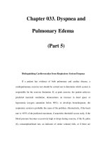
robot alignment experiments (Section 5.2.1). The trajectories of the robots can be seen in

Figure 1. The laser measurements have been used as ground truth in order to estimate the
accuracy of the results obtained.


Fig. 1. Trajectories performed by four Pioneer P3AT robots and a 2D view of the global map.

3. Map alignment

The main objective of this work is to study the alignment stage in a multi-robot visual SLAM
context. At the beginning, the robots start performing their navigation tasks independently,
and build local maps. Given two of these feature maps, computing the alignment means

computing the transformation, if existent, between those maps. In this way the landmarks
belonging to different maps are expressed into the same reference system. Initially, before
the alignment is performed, the local map of each robot is referred to its local reference
system which is located at the starting point of the robot.
In order to compute the transformation between local maps, some approaches try to
compute the relative poses of the robots. In this sense, the easiest case can be seen in (Thrun,
2001), where the relative pose of the robots is suppose to be known. A more challenging
approach is presented in (Konolige et al., 2003; Zhou & Roumeliotis, 2006). In these cases,
the robots, being in communication range, agree to meet at some point. If the meeting
succeed, then the robots share information and compute their relative poses. Other
approaches present feature-based techniques in order to align maps (Se et al., 2005; Thrun &
Liu, 2004). The basis of these techniques is to find matches between the landmarks of the
local maps and then to obtain the transformation between them. This paper focuses on the
last approach.
In our case, although the maps are 3D, the alignment is performed in 2D. This is due to the
fact that the robots’ movements are performed in a 2D plane. The result of the alignment is a
translation in x and y (t
x
and t
y
) and a rotation θ. This can be expressed as a transformation
matrix T:

Evaluationofaligningmethodsforlandmark-basedmapsinvisualSLAM 135

we focus on this approach. In this context, two main proposals can be found in the
literature. On the one hand, there are some solutions in which the estimate of the maps and
trajectories is performed jointly (Fenwick et al., 2002; Gil et al., 2007; Thrun & Liu, 2004). In
this case, there is a unique map, which is simultaneous built from the observations of the
robots. In this way, the robots have a global notion of the unexplored areas so that the

cooperative exploration can be improved. Moreover, in a feature-based SLAM, a landmark
can be updated by different robots in such a way that the robots do not need to revisit a
previously explored area in order to close the loop and reduce its uncertainty. However, the
maintenance of this global map can be computationally expensive and the initial position of
the robots should be known, which may not be possible in practice.
On the other hand, some approaches consider the case in which each robot builds a local
map independently (Stewart et al., 2003; Zhou & Roumeliotis, 2006). Then, at some point
the robots may decide to fuse their maps into a global one. In (Stewart et al., 2003), there is
some point where the robots arrange to meet in. At that point, the robots can compute their
relative positions and fuse their maps. One of the main advantages of using independent
local maps, as explained in (Williams, 2001), is that the data association problem is
improved. First, new observations should be only matched with a reduced number of
landmarks in the map. Moreover, when these landmarks are fused into a global map, a more
robust data association can be performed between the local maps. However, one of the
drawbacks of this approach is dealing with the uncertainty of the local maps built by
different robots when merging them.
The map fusion problem can be divided into two subproblems: the map alignment and the
fusion of the data. The first stage consists in computing the transformation between the local
maps, which have different reference systems. Next, after expressing all the landmarks in
the same reference system, the data can be fused into a global map. In this work, we focus
on the alignment problem in a multirobot visual SLAM context.

2. Map Building

The experiments have been carried out with Pioneer-P3AT robots, provided with a laser
sensor and STH-MDCS2 stereo head from Videre Design. The stereo cameras have been
previously calibrated and obtain 3D information from the environment. The maps thus
built, are made of visual landmarks. These visual landmarks consist of the 3D position of the
distinctive points extracted by the Harris Corner detector (Harris & Stephens, 1998). These
points have an associated covariance matrix representing the uncertainty in the estimate of

the landmarks. Furthermore these points are characterized by the U-SURF descriptor (Bay et
al., 2006). The selection of the Harris Corner detector combined with the U-SURF descriptor
is the result of a previous work, in which the aim was to find a suitable feature extractor for
visual SLAM (Ballesta et al., 2007; Martinez Mozos et al., 2007; Gil et al., 2009).
The robots start at different positions and perform different trajectories in a 2D plane,
sharing a common space in a typical office building. The maps are built with the FastSLAM
algorithm using exclusively visual information. Laser readings are used as ground truth.
The number of particles selected for the FastSLAM algorithm is M=200.
The alignment experiments have been initially carried out using two maps from two
different robots (Section 5.1 and 5.2). Then, four different maps were used for the multi-
robot alignment experiments (Section 5.2.1). The trajectories of the robots can be seen in

Figure 1. The laser measurements have been used as ground truth in order to estimate the
accuracy of the results obtained.


Fig. 1. Trajectories performed by four Pioneer P3AT robots and a 2D view of the global map.

3. Map alignment

The main objective of this work is to study the alignment stage in a multi-robot visual SLAM
context. At the beginning, the robots start performing their navigation tasks independently,
and build local maps. Given two of these feature maps, computing the alignment means
computing the transformation, if existent, between those maps. In this way the landmarks
belonging to different maps are expressed into the same reference system. Initially, before
the alignment is performed, the local map of each robot is referred to its local reference
system which is located at the starting point of the robot.
In order to compute the transformation between local maps, some approaches try to
compute the relative poses of the robots. In this sense, the easiest case can be seen in (Thrun,
2001), where the relative pose of the robots is suppose to be known. A more challenging

approach is presented in (Konolige et al., 2003; Zhou & Roumeliotis, 2006). In these cases,
the robots, being in communication range, agree to meet at some point. If the meeting
succeed, then the robots share information and compute their relative poses. Other
approaches present feature-based techniques in order to align maps (Se et al., 2005; Thrun &
Liu, 2004). The basis of these techniques is to find matches between the landmarks of the
local maps and then to obtain the transformation between them. This paper focuses on the
last approach.
In our case, although the maps are 3D, the alignment is performed in 2D. This is due to the
fact that the robots’ movements are performed in a 2D plane. The result of the alignment is a
translation in x and y (t
x
and t
y
) and a rotation θ. This can be expressed as a transformation
matrix T:

RobotLocalizationandMapBuilding136


















1000
0100
0cossin
0sincos
y
x
t
t
T





(1)
Given two maps m and m’, T transforms the reference system of m’ into the reference
system of m.
In order to select an adequate method to align this kind of maps, we have performed a
comparative evaluation of a set of aligning methods (Section 4). All these methods try to
establish correspondences between the local maps by means of the descriptor similarity.
Furthermore, we have divided this study into to stages: first with simulated data (Section
5.1) and then with real data captured by the robots (Section 5.2). These experiments are
performed between pairs of maps. However, we have additionally considered the multi-
robot case, in which the number of robots is higher than 2. In this case, the alignment should
be consistent, not only between pair of maps but also globally. This is explained in detail in
the next section (Section 3.1).

3.1 Multi-robot alignment
This section tackles the problem in which there are n robots (n>2) whose maps should be
aligned. In this case, the alignment should be consistent not only between pairs of maps but
also globally. In order to deal with this situation, some constraints should be established (Se
et al., 2005).
First, given n maps (n>2) and having each pair of them an overlapping part, the following
constraint should be satisfied in the ideal case:

T
1
·T
2
·…·T
n
= I

(2)

where I is a 3X3 identity matrix. Each T
i
is the transformation matrix between map
i
and
map
i+1
and corresponds to the matrix in Equation 1. The particular case of T
n
refers to the
transformation matrix between map

n
and map
1
. The equation 2 leads to three expressions
that should be minimized:
E1. sin(θ
1
+…+ θ
n
)
E2. t
x1
+ t
x2
cos(θ
1
) + t
y2
sin(θ
1
) + t
x3
cos(θ
1
+θ
2
) + t
y3
sin(θ
1

+θ
2
) + … + t
xn
cos(θ
1
+…+θ
n-1
) +
t
yn
sin(θ
1
+…+θ
n-1
)
E2. t
y1
+ t
x2
sin(θ
1
) + t
y2
cos(θ
1
) - t
x3
sin(θ
1

+θ
2
) + t
y3
cos(θ
1
+θ
2
) + … - t
xn
sin(θ
1
+…+θ
n-1
) +
t
yn
cos(θ
1
+…+θ
n-1
)
Additionally, given a set of corresponding landmarks between map
i
and map
i+1
, and having
been aligned the landmarks of map
i+1
(L

j
) into map
1
’s coordinate system with the
transformation matrix T
i
(see Equation 1), the following expression should be minimized:

L
Aj{m{k}}
-L
i{m(k)}
(3)

where m(k) is the total number of correspondences between the k-pair of maps (kЄ{1,n}).
The number of equations that emerge from Equation 3 is 2m(1)+2m(2)+…+2m(n). For
instance, if we have m(1) common landmarks between map
1
and map
2
and the

transformation matrix between them is T
1
, then for each common landmark we should
minimize the following set of expressions:
Eδ. x2cos(θ
1
)+y2sin(θ
1

)+tx1-x1 with δ Є {4,X+4}
Eλ. y2cos(θ
1
)-x2sin(θ
1
)+ty1-y1 with λ Є {X+5,3X+5}
where X=m(1)+m(2)+…+m(n)
So far, we have a non-linear system of S = 3 + 2m(1) +…+ 2m(n) constraints that we should
minimize. In order to obtain the aligning parameters that minimize the previous S
constraints, we used the fsolve MATLAB function. This iterative algorithm uses a subspace
trust-region method which is based on the interior-reflective Newton method described in
(Coleman, 1994; Coleman, 1996). The input for this algorithm is an initial estimate of the
aligning parameters. This is obtained by the RANSAC algorithm of Sec. 4.1 between each
pair of maps, i.e., map
1
-map
2
, map
2
-map
3
, map
3
-map
4
and map
4
-map
1
. This will be the

starting point of the results obtained with fsolve function to find a final solution.

4. Aligning methods

4.1 RANSAC (Random Sample Consensus)
This algorithm has been already aplied to the map alignment problem in (Se et al., 2005).
The algorithm is performed as follows.
(a) In the first step, a list of possible corresponedences is obtained. The matching between
landmarks of both maps in done based on the Euclidean distance between their associated
descriptors d
i
. This distance should be the minimum and below a threshold th
0
= 0.7. As a
result of this first step, we obtain a list of matches consisting of the landmarks of one of the
maps and their correspondences in the other map, i.e., m and m’.
(b) In a second step, two pair of correspondences ([(x
i
,y
i
,z
i
),(x
i
’,y
i
’,z
i
’)]) are selected at random
from the previous list. These pairs should satisfy the following geometric constraint (Se et

al., 2005):

|(A
2
+ B
2
)-(C
2
+D
2
)|<th
1

(4)

where A = (x
i
’-x
j
’), B = (yi’-yj’), C = (xi-xj) and D = (yi-yj) . We have set the threshold th
1
= 0.8
m. The two pairs of correspondences are used to compute the alignment parameters (t
x
, t
y
, θ)
with the following equations:

t

x
= x
i
– x
i
’cosθ – y
i
’ sinθ

(5)

t
y
= y
i
– y
i
’cosθ + x
i
’ sinθ

(6)

θ = arctan((BC-AD)/(AC+BD))

(7)

(c) The third step consist in looking for correspondences that support the solution obtained
(t
x

, t
y
, θ). Concretely, we transform the landmarks of the second map using the alignment
obtained, so that it is referred to the same references system as the first map. Then, for each
landmark of the transformed map, we find the closest landmark of the first map in terms of
the Euclidean distance between their positions. The pairing is done if this distance is the
Evaluationofaligningmethodsforlandmark-basedmapsinvisualSLAM 137

















1000
0100
0cossin
0sincos
y
x

t
t
T





(1)
Given two maps m and m’, T transforms the reference system of m’ into the reference
system of m.
In order to select an adequate method to align this kind of maps, we have performed a
comparative evaluation of a set of aligning methods (Section 4). All these methods try to
establish correspondences between the local maps by means of the descriptor similarity.
Furthermore, we have divided this study into to stages: first with simulated data (Section
5.1) and then with real data captured by the robots (Section 5.2). These experiments are
performed between pairs of maps. However, we have additionally considered the multi-
robot case, in which the number of robots is higher than 2. In this case, the alignment should
be consistent, not only between pair of maps but also globally. This is explained in detail in
the next section (Section 3.1).

3.1 Multi-robot alignment
This section tackles the problem in which there are n robots (n>2) whose maps should be
aligned. In this case, the alignment should be consistent not only between pairs of maps but
also globally. In order to deal with this situation, some constraints should be established (Se
et al., 2005).
First, given n maps (n>2) and having each pair of them an overlapping part, the following
constraint should be satisfied in the ideal case:

T

1
·T
2
·…·T
n
= I

(2)

where I is a 3X3 identity matrix. Each T
i
is the transformation matrix between map
i
and
map
i+1
and corresponds to the matrix in Equation 1. The particular case of T
n
refers to the
transformation matrix between map
n
and map
1
. The equation 2 leads to three expressions
that should be minimized:
E1. sin(θ
1
+…+ θ
n
)

E2. t
x1
+ t
x2
cos(θ
1
) + t
y2
sin(θ
1
) + t
x3
cos(θ
1
+θ
2
) + t
y3
sin(θ
1
+θ
2
) + … + t
xn
cos(θ
1
+…+θ
n-1
) +
t

yn
sin(θ
1
+…+θ
n-1
)
E2. t
y1
+ t
x2
sin(θ
1
) + t
y2
cos(θ
1
) - t
x3
sin(θ
1
+θ
2
) + t
y3
cos(θ
1
+θ
2
) + … - t
xn

sin(θ
1
+…+θ
n-1
) +
t
yn
cos(θ
1
+…+θ
n-1
)
Additionally, given a set of corresponding landmarks between map
i
and map
i+1
, and having
been aligned the landmarks of map
i+1
(L
j
) into map
1
’s coordinate system with the
transformation matrix T
i
(see Equation 1), the following expression should be minimized:

L
Aj{m{k}}

-L
i{m(k)}

(3)

where m(k) is the total number of correspondences between the k-pair of maps (kЄ{1,n}).
The number of equations that emerge from Equation 3 is 2m(1)+2m(2)+…+2m(n). For
instance, if we have m(1) common landmarks between map
1
and map
2
and the

transformation matrix between them is T
1
, then for each common landmark we should
minimize the following set of expressions:
Eδ. x2cos(θ
1
)+y2sin(θ
1
)+tx1-x1 with δ Є {4,X+4}
Eλ. y2cos(θ
1
)-x2sin(θ
1
)+ty1-y1 with λ Є {X+5,3X+5}
where X=m(1)+m(2)+…+m(n)
So far, we have a non-linear system of S = 3 + 2m(1) +…+ 2m(n) constraints that we should
minimize. In order to obtain the aligning parameters that minimize the previous S

constraints, we used the fsolve MATLAB function. This iterative algorithm uses a subspace
trust-region method which is based on the interior-reflective Newton method described in
(Coleman, 1994; Coleman, 1996). The input for this algorithm is an initial estimate of the
aligning parameters. This is obtained by the RANSAC algorithm of Sec. 4.1 between each
pair of maps, i.e., map
1
-map
2
, map
2
-map
3
, map
3
-map
4
and map
4
-map
1
. This will be the
starting point of the results obtained with fsolve function to find a final solution.

4. Aligning methods

4.1 RANSAC (Random Sample Consensus)
This algorithm has been already aplied to the map alignment problem in (Se et al., 2005).
The algorithm is performed as follows.
(a) In the first step, a list of possible corresponedences is obtained. The matching between
landmarks of both maps in done based on the Euclidean distance between their associated

descriptors d
i
. This distance should be the minimum and below a threshold th
0
= 0.7. As a
result of this first step, we obtain a list of matches consisting of the landmarks of one of the
maps and their correspondences in the other map, i.e., m and m’.
(b) In a second step, two pair of correspondences ([(x
i
,y
i
,z
i
),(x
i
’,y
i
’,z
i
’)]) are selected at random
from the previous list. These pairs should satisfy the following geometric constraint (Se et
al., 2005):

|(A
2
+ B
2
)-(C
2
+D

2
)|<th
1

(4)

where A = (x
i
’-x
j
’), B = (yi’-yj’), C = (xi-xj) and D = (yi-yj) . We have set the threshold th
1
= 0.8
m. The two pairs of correspondences are used to compute the alignment parameters (t
x
, t
y
, θ)
with the following equations:

t
x
= x
i
– x
i
’cosθ – y
i
’ sinθ

(5)

t
y
= y
i
– y
i
’cosθ + x
i
’ sinθ

(6)

θ = arctan((BC-AD)/(AC+BD))

(7)

(c) The third step consist in looking for correspondences that support the solution obtained
(t
x
, t
y
, θ). Concretely, we transform the landmarks of the second map using the alignment
obtained, so that it is referred to the same references system as the first map. Then, for each
landmark of the transformed map, we find the closest landmark of the first map in terms of
the Euclidean distance between their positions. The pairing is done if this distance is the
RobotLocalizationandMapBuilding138

minimum and is below the threshold th

2
=0.4m. As a result, we will have a set of matches
that support the solution of the alignment.
(d) Finally, steps (c) and (d) are repeated M=70 times. The final solution will be that one
with the highest number of supports.
In this algorithm, we have defined three different thresholds: th
0
=0.7 for the selection of the
initial correspondences, th
1
=0.8 for the geometric constraint of Equation 4 and th
2
=0.4m for
selecting supports. Furthermore, a parameter min =20 establishes the minimum number of
supports in order to validae a solution and M=70 is the number of times that steps (c) and
(d) are repeated. These are considered as internal parameters of the algorithm and their
values have been experimentally selected.

4.2 SVD (Singular Value Decomposition)
One of the applications of the Singular Value Decomposition (SVD) is the registration of 3D
point sets (Arun et al., 1987; Rieger, 1987). The registration consists in obtaining a common
reference frame by estimating the transformations between the datasets. In this work the
SVD has been applied for the computation of the alignment between two maps. We first
compute a list of correspondences. In order to construct this list (m, m’), we impose two
different constraints. The first one is tested by performing the first step of the RANSAC
algorithm (Section 4.1). In addition, the geometric constraint of Equation 4 is evaluated.
Given this list of possible correspondences, our aim is to minimize the following expression:

||Tm’-m||

(8)

where m are the landmarks of one of the maps and m’ their correspondences in the other
map. On the other hand, T is the transformation matrix between both coordinate systems
(Equation 1). T is computed as shown in Algorithm 1 of this section.

Algorithm 1.
Computation of T, given m and m’
1: [u,d,v] = svd(m’)
2: z=u
T
m
3: sv=diag(d)
4: z
1
=z(1:n) {n is the Lumber of eigenvalues (not equal to 0) in sv}
5: w=z
1
./sv
6: T=(v*w)
T

4.3 ICP (Iterated Closest Point)
The Iterative Closest Point (ICP) technique was introduced in (Besl & McKay, 1992; Zhang,
1992) and applied to the task of point registration. The ICP algorithm consists of two steps
that are iterated:
(a) Compute correspondences (m, m’). Given an initial estimate T
0
, a set of correspondences
(m,m’) is computed, so that it supports the initial parameters T

0
. T
0
is the transformation
matrix between both maps and is computed with Equations 5, 6 and 7.
(b) Update transformation T. The previous set of correspondences is used to update the
transformation T. The new T
x+1
will minimize the expression: ||T
x+1
·m’-m||, which is

analogous to the expression (5). For this reason, we have solved this step with the SVD
algorithm (Algorithm 1).
The algorithm stops when the set of correspondences does not change in the first step, and
therefore T
x+1
is equal to T in the second step.
This technique needs an accurate initial estimation of the transformation parameters so that
it converges properly. For that reason, in order to obtain an appropriate initial estimate we
perform the two first steps in RANSAC algorithm (Section 4.1). The same threshold values
are used.

4.4 ImpICP (Improved Iterated Closest Point)
The improved ICP (ImpICP) method is a modification of the ICP algorithm presented in
Section 4.3, which has been implemented ad hoc. This new version is motivated by the
importance of obtaining a precise initial estimation of the transformation parameter T
0
. The
accuracy of the results obtained is highly dependent on the goodness of this initial estimate.

For that reason, in this new version of the ICP algorithm, we have increased the probability
of obtaining a desirable result. Particularly, we obtain three different initial estimates instead
of only one. This is performed by selecting three different pairs of correspondences each
case in the second step of the RANSAC algorithm (Section 4.1), leading to three initial
estimates. For each initial estimate, the algorithm runs as in Section 4.3. Finally, the solution
selected is the transformation that is supported by a highest number of correspondences.

5. Experiments

The aim of this work is to find a suitable aligning method so that two or more maps can be
expressed in the same reference system. This method should be appropriate for the kind of
maps that our robots build, that is to say, landmark-based maps. With this idea, we have
selected a set of algorithms that satisfy this requirement (See Section 4).
In order to perform these experiments, we have organised the work in two stages: first, a
comparison of the aligning methods selected, using simulated data. In this case, we vary the
amount of noise of the input data and observe the results by aligning pairs of maps. Secondly,
we repeated the same experiments using real data captured by the robots. Furthermore, we
include an experiment showing the performance of the multi-alignment case explained in
Section 3.1, in which the number of maps we want to align is higher than 2.

5.1 Simulated Data
In order to perform the comparison between the aligning methods, we have built two 3D
feature maps as can be seen in Figure 2. The coordinates of the landmarks have been
simulated so that the alignment is evaluated with independence of the uncertainty in the
estimate of the landmarks. Then, these points are described by U-SURF, extracted from real
images which are typical scenarios of our laboratory. map
1
from Figure 2 has 250 points
(stars), whereas map2 (circles) has a common area with map
1

, whose size is variable, and a
non-overlapping part which has 88 points. During the experimental performance, we test
with different sizes of the overlapping area between these two maps (pentagons), so that we
can observe the performance of the aligning methods vs. different levels of coincidence
between the maps.
Evaluationofaligningmethodsforlandmark-basedmapsinvisualSLAM 139

minimum and is below the threshold th
2
=0.4m. As a result, we will have a set of matches
that support the solution of the alignment.
(d) Finally, steps (c) and (d) are repeated M=70 times. The final solution will be that one
with the highest number of supports.
In this algorithm, we have defined three different thresholds: th
0
=0.7 for the selection of the
initial correspondences, th
1
=0.8 for the geometric constraint of Equation 4 and th
2
=0.4m for
selecting supports. Furthermore, a parameter min =20 establishes the minimum number of
supports in order to validae a solution and M=70 is the number of times that steps (c) and
(d) are repeated. These are considered as internal parameters of the algorithm and their
values have been experimentally selected.

4.2 SVD (Singular Value Decomposition)
One of the applications of the Singular Value Decomposition (SVD) is the registration of 3D
point sets (Arun et al., 1987; Rieger, 1987). The registration consists in obtaining a common
reference frame by estimating the transformations between the datasets. In this work the

SVD has been applied for the computation of the alignment between two maps. We first
compute a list of correspondences. In order to construct this list (m, m’), we impose two
different constraints. The first one is tested by performing the first step of the RANSAC
algorithm (Section 4.1). In addition, the geometric constraint of Equation 4 is evaluated.
Given this list of possible correspondences, our aim is to minimize the following expression:

||Tm’-m||

(8)

where m are the landmarks of one of the maps and m’ their correspondences in the other
map. On the other hand, T is the transformation matrix between both coordinate systems
(Equation 1). T is computed as shown in Algorithm 1 of this section.

Algorithm 1. Computation of T, given m and m’
1: [u,d,v] = svd(m’)
2: z=u
T
m
3: sv=diag(d)
4: z
1
=z(1:n) {n is the Lumber of eigenvalues (not equal to 0) in sv}
5: w=z
1
./sv
6: T=(v*w)
T

4.3 ICP (Iterated Closest Point)

The Iterative Closest Point (ICP) technique was introduced in (Besl & McKay, 1992; Zhang,
1992) and applied to the task of point registration. The ICP algorithm consists of two steps
that are iterated:
(a) Compute correspondences (m, m’). Given an initial estimate T
0
, a set of correspondences
(m,m’) is computed, so that it supports the initial parameters T
0
. T
0
is the transformation
matrix between both maps and is computed with Equations 5, 6 and 7.
(b) Update transformation T. The previous set of correspondences is used to update the
transformation T. The new T
x+1
will minimize the expression: ||T
x+1
·m’-m||, which is

analogous to the expression (5). For this reason, we have solved this step with the SVD
algorithm (Algorithm 1).
The algorithm stops when the set of correspondences does not change in the first step, and
therefore T
x+1
is equal to T in the second step.
This technique needs an accurate initial estimation of the transformation parameters so that
it converges properly. For that reason, in order to obtain an appropriate initial estimate we
perform the two first steps in RANSAC algorithm (Section 4.1). The same threshold values
are used.

4.4 ImpICP (Improved Iterated Closest Point)
The improved ICP (ImpICP) method is a modification of the ICP algorithm presented in
Section 4.3, which has been implemented ad hoc. This new version is motivated by the
importance of obtaining a precise initial estimation of the transformation parameter T
0
. The
accuracy of the results obtained is highly dependent on the goodness of this initial estimate.
For that reason, in this new version of the ICP algorithm, we have increased the probability
of obtaining a desirable result. Particularly, we obtain three different initial estimates instead
of only one. This is performed by selecting three different pairs of correspondences each
case in the second step of the RANSAC algorithm (Section 4.1), leading to three initial
estimates. For each initial estimate, the algorithm runs as in Section 4.3. Finally, the solution
selected is the transformation that is supported by a highest number of correspondences.

5. Experiments

The aim of this work is to find a suitable aligning method so that two or more maps can be
expressed in the same reference system. This method should be appropriate for the kind of
maps that our robots build, that is to say, landmark-based maps. With this idea, we have
selected a set of algorithms that satisfy this requirement (See Section 4).
In order to perform these experiments, we have organised the work in two stages: first, a
comparison of the aligning methods selected, using simulated data. In this case, we vary the
amount of noise of the input data and observe the results by aligning pairs of maps. Secondly,
we repeated the same experiments using real data captured by the robots. Furthermore, we
include an experiment showing the performance of the multi-alignment case explained in
Section 3.1, in which the number of maps we want to align is higher than 2.

5.1 Simulated Data
In order to perform the comparison between the aligning methods, we have built two 3D
feature maps as can be seen in Figure 2. The coordinates of the landmarks have been

simulated so that the alignment is evaluated with independence of the uncertainty in the
estimate of the landmarks. Then, these points are described by U-SURF, extracted from real
images which are typical scenarios of our laboratory. map
1
from Figure 2 has 250 points
(stars), whereas map2 (circles) has a common area with map
1
, whose size is variable, and a
non-overlapping part which has 88 points. During the experimental performance, we test
with different sizes of the overlapping area between these two maps (pentagons), so that we
can observe the performance of the aligning methods vs. different levels of coincidence
between the maps.
RobotLocalizationandMapBuilding140

map
2
is 0.35 rads rotated and t
x
= 5m, t
y
= 10 m translated from map1. The size of the maps
is 30X30 metres. Coincident points between the maps have initially the same descriptors.
However, a Gaussian noise has been added to map2 so that the data are closer to reality. As
a consequence, map2 has noise with σL in the localization of the points (coordinates’
estimate) and noise with σD in the descriptors. The magnitude of σL and σD has been
chosen experimentally.


Fig. 2. 2D view of map1 and map2 (simulated data).

Figures 3, 4, 5 and 6 represent the results obtained with a noise of σL and σD equal to 0.20,
whereas in Figures 7, 8, 9 and 10 these values are 0.50. In the X-axis, the number of points
that both maps have in common is represented. This value varies from 0 to 160. The first
value shows the case in which the maps do not overlap at all. For each value, the experiment
is repeated 10 times. Then the Mean Quadratic Error is shown in the Y-axis (blue line). This
value is computed comparing the alignment obtained and a ground truth. The blue points
represent the individual values of the Error in each one of the 10 repetitions. In a similar
way, the number of supports is also included in the graphics (red points). The number of
supports is the number of correspondences that satisfy the transformation obtained. The
mean value of supports is represented with a red line. In Figures 3 and 7, the green line
represents the minimum value of supports required to validate the solution. Finally, all the
figures present with bars the number of failures obtained in the 10 repetitions. Each failure
represents the case in which the method does not converge to any solution or the solution
does not satisfy the requirements (RANSAC method). In these cases, we consider that no
alignment has been found.
Figures 3 and 7 show the results obtained with the RANSAC algorithm of Sec. 4.1. In figure
3, no solution is obtained until the number of overlapping points is higher than 60 points. In
all of those cases, the Mean Quadratic Error always below 2 m. Regarding the number of
supports (red line), we observe an ascendant tendency due to the increasing number of
overlapping points. In the case of 160 overlapping points, the number of supports is 80. If
the Gaussian noise is higher, these results get worse, as in Figure 7 where the number of
supports obtained is significantly lower. Furthermore, the first solution appears when the
number of overlapping points is 120.

Figures 4 and 8 present the results of the SVD algorithm of Section 4.2. In those cases, the
error value having 100 overlapping points is close to 30. At least, the error has a descendent
tendency as the number of overlapping points increases. However, in Fig 8 the error values
are much more unstable. Regarding the number of supports, the tendency is quite constant
in both graphics.
The behaviour of the ICP algorithm of Section 4.3 is presented in Figs. 5 and 9. In Figure 5

the error value obtained is quite acceptable. It is noticeable that the error curve decreases
sharply from the case of 20 to 60 overlapping points. Then, the curve continues descending
very slightly. This last part of the curve shows that the error values are around 2, which is a
quite good result. Nevertheless, the yellow bars show, in some cases, a small number of
failures. Fig. 9 shows worse results.
Finally, in Figures 6 and 10, the results of the improved version of ICP are shown. In this
case, the results obtained are similar to that of ICP in terms of mean support values.
However, it is noticeable that the stability of the algorithm is higher. If we pay attention to
the yellow bars in Figure 6, it is shown that the algorithm always obtains a solution when
the number of overlapping points is equal or higher than 100. In Figure 10, the number of
failures is lower than in Figure 9.
In general, the best results are obtained by the ImpICP and RANSAC algorithms. RANSAC
obtains lower error values, whereas ImpICP is more stable in terms of having less number of
failures.
In addition to the experiments performed to evaluate the accuracy and suitability of the
aligning methods, we have also measured the computational time of each algorithm (see
Figure 11). The curves show an ascendant tendency. This is due to the fact that the size of
map2 is higher as the number of overlapping points increases. It is remarkable that the
values of the computation time are very similar in all of the methods. For that reason, this
criterion can not be used to select one of the methods.


Fig. 3. RANSAC algorithm. The Gaussian noise is σ
D
= σ
L
= 0.20.
Evaluationofaligningmethodsforlandmark-basedmapsinvisualSLAM 141

map

2
is 0.35 rads rotated and t
x
= 5m, t
y
= 10 m translated from map1. The size of the maps
is 30X30 metres. Coincident points between the maps have initially the same descriptors.
However, a Gaussian noise has been added to map2 so that the data are closer to reality. As
a consequence, map2 has noise with σL in the localization of the points (coordinates’
estimate) and noise with σD in the descriptors. The magnitude of σL and σD has been
chosen experimentally.


Fig. 2. 2D view of map1 and map2 (simulated data).

Figures 3, 4, 5 and 6 represent the results obtained with a noise of σL and σD equal to 0.20,
whereas in Figures 7, 8, 9 and 10 these values are 0.50. In the X-axis, the number of points
that both maps have in common is represented. This value varies from 0 to 160. The first
value shows the case in which the maps do not overlap at all. For each value, the experiment
is repeated 10 times. Then the Mean Quadratic Error is shown in the Y-axis (blue line). This
value is computed comparing the alignment obtained and a ground truth. The blue points
represent the individual values of the Error in each one of the 10 repetitions. In a similar
way, the number of supports is also included in the graphics (red points). The number of
supports is the number of correspondences that satisfy the transformation obtained. The
mean value of supports is represented with a red line. In Figures 3 and 7, the green line
represents the minimum value of supports required to validate the solution. Finally, all the
figures present with bars the number of failures obtained in the 10 repetitions. Each failure
represents the case in which the method does not converge to any solution or the solution
does not satisfy the requirements (RANSAC method). In these cases, we consider that no
alignment has been found.

Figures 3 and 7 show the results obtained with the RANSAC algorithm of Sec. 4.1. In figure
3, no solution is obtained until the number of overlapping points is higher than 60 points. In
all of those cases, the Mean Quadratic Error always below 2 m. Regarding the number of
supports (red line), we observe an ascendant tendency due to the increasing number of
overlapping points. In the case of 160 overlapping points, the number of supports is 80. If
the Gaussian noise is higher, these results get worse, as in Figure 7 where the number of
supports obtained is significantly lower. Furthermore, the first solution appears when the
number of overlapping points is 120.

Figures 4 and 8 present the results of the SVD algorithm of Section 4.2. In those cases, the
error value having 100 overlapping points is close to 30. At least, the error has a descendent
tendency as the number of overlapping points increases. However, in Fig 8 the error values
are much more unstable. Regarding the number of supports, the tendency is quite constant
in both graphics.
The behaviour of the ICP algorithm of Section 4.3 is presented in Figs. 5 and 9. In Figure 5
the error value obtained is quite acceptable. It is noticeable that the error curve decreases
sharply from the case of 20 to 60 overlapping points. Then, the curve continues descending
very slightly. This last part of the curve shows that the error values are around 2, which is a
quite good result. Nevertheless, the yellow bars show, in some cases, a small number of
failures. Fig. 9 shows worse results.
Finally, in Figures 6 and 10, the results of the improved version of ICP are shown. In this
case, the results obtained are similar to that of ICP in terms of mean support values.
However, it is noticeable that the stability of the algorithm is higher. If we pay attention to
the yellow bars in Figure 6, it is shown that the algorithm always obtains a solution when
the number of overlapping points is equal or higher than 100. In Figure 10, the number of
failures is lower than in Figure 9.
In general, the best results are obtained by the ImpICP and RANSAC algorithms. RANSAC
obtains lower error values, whereas ImpICP is more stable in terms of having less number of
failures.
In addition to the experiments performed to evaluate the accuracy and suitability of the

aligning methods, we have also measured the computational time of each algorithm (see
Figure 11). The curves show an ascendant tendency. This is due to the fact that the size of
map2 is higher as the number of overlapping points increases. It is remarkable that the
values of the computation time are very similar in all of the methods. For that reason, this
criterion can not be used to select one of the methods.


Fig. 3. RANSAC algorithm. The Gaussian noise is σ
D
= σ
L
= 0.20.
RobotLocalizationandMapBuilding142


Fig. 4. ICP algorithm. The Gaussian noise is σ
D
= σ
L
= 0.20.


Fig. 5. SVD algorithm. The Gaussian noise is σ
D
= σ
L
= 0.20.

Fig. 6. ImpICP algorithm. The Gaussian noise is σ
D
= σ
L
= 0.20.


Fig. 7. RANSAC algorithm. The Gaussian noise is σ
D
= σ
L
= 0.50.

Evaluationofaligningmethodsforlandmark-basedmapsinvisualSLAM 143


Fig. 4. ICP algorithm. The Gaussian noise is σ
D
= σ
L
= 0.20.


Fig. 5. SVD algorithm. The Gaussian noise is σ
D
= σ
L
= 0.20.

Fig. 6. ImpICP algorithm. The Gaussian noise is σ
D
= σ
L
= 0.20.


Fig. 7. RANSAC algorithm. The Gaussian noise is σ
D
= σ
L
= 0.50.

RobotLocalizationandMapBuilding144


Fig. 8. ICP algorithm. The Gaussian noise is σ
D
= σ
L
= 0.50.


Fig. 9. SVD algorithm. The Gaussian noise is σ
D
= σ
L
= 0.50.

Fig. 10. ImpICP algorithm. The Gaussian noise is σ
D
= σ
L
= 0.50.


Fig. 11. Computational time vs. number of overlapping points.

5.2 Real Data
After performing the comparative analysis with the simulated data, the next step is to
evaluate the same aligning methods using real data captured by the robots, i.e., landmarks
consisting of Harris points detected from the environment and described by U-SURF.
Evaluationofaligningmethodsforlandmark-basedmapsinvisualSLAM 145


Fig. 8. ICP algorithm. The Gaussian noise is σ
D
= σ
L
= 0.50.


Fig. 9. SVD algorithm. The Gaussian noise is σ
D
= σ
L
= 0.50.

Fig. 10. ImpICP algorithm. The Gaussian noise is σ
D
= σ
L
= 0.50.


Fig. 11. Computational time vs. number of overlapping points.

5.2 Real Data
After performing the comparative analysis with the simulated data, the next step is to
evaluate the same aligning methods using real data captured by the robots, i.e., landmarks
consisting of Harris points detected from the environment and described by U-SURF.
RobotLocalizationandMapBuilding146

We evaluate the performance of the aligning methods at different steps of the mapping
process, i.e., at different iterations of the FastSLAM algorithm. At the beginning, the maps
built by each robot have a reduced number of landmarks and therefore there are fewer
possibilities of finding correspondences between these local maps. However, this situation
changes as long as the maps are bigger. In this situation the probability of finding
correspondences is higher and it is expected to obtain the alignment successfully.
In these experiments we have used the most probable map of each robot in order to
compute the transformation between their reference systems. We obtain the most probable
map of each robot at different iterations of the FastSLAM algorithm and try to align these
maps. The most probable map is the map of the most probable particle of the filter in each
particular moment.
The FastSLAM algorithm is performed in several iterations corresponding to the total

number of movements performed by the robot. In the experiments k is an index that denotes
the number of iterations. In this case, this number is k=1410 and the sizes of the maps at that
point are map
1
=263 landmarks and map
2
=346 landmarks. These maps have a dimension of
35X15 meters approximately.
In Figure 15(a), we can observe a 2D view of the local maps constructed by each robot and
referred to its local frame. In this figure, map
1
is represented by stars and has 181
landmarks. On the other hand, map
2
is represented by circles and it size is of 187 landmarks.
In Figure 15(b), we can see the two local maps already aligned. In this case, the most
probable maps of iteration k=810 have been used.
In order to compare the aligning methods with real data, we compute the alignment
parameters for each method at different iterations of the FastSLAM algorithm. The
evaluating measure is the Euclidean distance between the alignment parameters tx,ty and θ
the real relative position between the robots, denoted as ground truth. This measure was
obtained estimating the relative position of the robots being at their starting positions.
Figure 12, illustrates the comparison of the aligning methods we evaluate. For each method,
the error values (y axis) vs. the k-iteration of the algorithm (x axis) are represented.
Logically, as the number of iterations increases, the size of the maps constructed will be
higher and therefore it will be more probable to find a solution closer to the ground truth.
For this reason, it is expected to obtain small error values as the k-iteration increases. In
Figure 12 we can observe that the worst results are obtained with SVD. For instance, SVD
has an error of 4m with k-iteration =1409, i.e., at the end of the FasSLAM algorithm. Next,
ICP obtains similar results. However, it achieves better results in some cases. For example,

with k-iteration = 810 the error is lower than 1 m. Then, the ImpICP algorithm outperforms
these previous methods, since it achieves really small error values. Nevertheless, RANSAC
is the method that obtains better results. Despite the fact that it gives no solution with k-
iteration = 60 (probably because the maps are still too sparse in this iteration), the algorithm
obtains the smallest error values. In fact, from k-iteration =410 on the error is no higher than
0.5m. Finally, Figures 13 and 14 focus on the results obtained by the RANSAC algorithm.
Figure 13 shows the number of supports obtained in each case, which increases with the k-
iteration values. On the other hand, Figure 14 shows the decomposition of the error in its
three components (three alignment parameteres): error in tx, ty and θ.



Fig. 12. Evaluation of the aligning methods.


Fig. 13. Results obtained with the RANSAC algorithm. Number of supports.


Fig. 14. Results obtained with the RANSAC algorithm. Error values for each aligning
parameter.
Evaluationofaligningmethodsforlandmark-basedmapsinvisualSLAM 147

We evaluate the performance of the aligning methods at different steps of the mapping
process, i.e., at different iterations of the FastSLAM algorithm. At the beginning, the maps
built by each robot have a reduced number of landmarks and therefore there are fewer
possibilities of finding correspondences between these local maps. However, this situation
changes as long as the maps are bigger. In this situation the probability of finding
correspondences is higher and it is expected to obtain the alignment successfully.
In these experiments we have used the most probable map of each robot in order to
compute the transformation between their reference systems. We obtain the most probable

map of each robot at different iterations of the FastSLAM algorithm and try to align these
maps. The most probable map is the map of the most probable particle of the filter in each
particular moment.
The FastSLAM algorithm is performed in several iterations corresponding to the total
number of movements performed by the robot. In the experiments k is an index that denotes
the number of iterations. In this case, this number is k=1410 and the sizes of the maps at that
point are map
1
=263 landmarks and map
2
=346 landmarks. These maps have a dimension of
35X15 meters approximately.
In Figure 15(a), we can observe a 2D view of the local maps constructed by each robot and
referred to its local frame. In this figure, map
1
is represented by stars and has 181
landmarks. On the other hand, map
2
is represented by circles and it size is of 187 landmarks.
In Figure 15(b), we can see the two local maps already aligned. In this case, the most
probable maps of iteration k=810 have been used.
In order to compare the aligning methods with real data, we compute the alignment
parameters for each method at different iterations of the FastSLAM algorithm. The
evaluating measure is the Euclidean distance between the alignment parameters tx,ty and θ
the real relative position between the robots, denoted as ground truth. This measure was
obtained estimating the relative position of the robots being at their starting positions.
Figure 12, illustrates the comparison of the aligning methods we evaluate. For each method,
the error values (y axis) vs. the k-iteration of the algorithm (x axis) are represented.
Logically, as the number of iterations increases, the size of the maps constructed will be
higher and therefore it will be more probable to find a solution closer to the ground truth.

For this reason, it is expected to obtain small error values as the k-iteration increases. In
Figure 12 we can observe that the worst results are obtained with SVD. For instance, SVD
has an error of 4m with k-iteration =1409, i.e., at the end of the FasSLAM algorithm. Next,
ICP obtains similar results. However, it achieves better results in some cases. For example,
with k-iteration = 810 the error is lower than 1 m. Then, the ImpICP algorithm outperforms
these previous methods, since it achieves really small error values. Nevertheless, RANSAC
is the method that obtains better results. Despite the fact that it gives no solution with k-
iteration = 60 (probably because the maps are still too sparse in this iteration), the algorithm
obtains the smallest error values. In fact, from k-iteration =410 on the error is no higher than
0.5m. Finally, Figures 13 and 14 focus on the results obtained by the RANSAC algorithm.
Figure 13 shows the number of supports obtained in each case, which increases with the k-
iteration values. On the other hand, Figure 14 shows the decomposition of the error in its
three components (three alignment parameteres): error in tx, ty and θ.



Fig. 12. Evaluation of the aligning methods.


Fig. 13. Results obtained with the RANSAC algorithm. Number of supports.


Fig. 14. Results obtained with the RANSAC algorithm. Error values for each aligning
parameter.
RobotLocalizationandMapBuilding148


(a) (b)
Fig. 15. Map alignment with real data. (a) Local maps before de alignment. Example of
detected correspondences. (b) Map after the alignment.

5.2.1 Multi-alignment results.
Table 1 presents an example of the results obtained with the fsolve function (Section 3.1).
This table shows the aligning results obtained in the group of four robots, where T
i
j

represents the alignment between robot i and robot j. On the top part of the table, we can
observe the aligning results between each pair of robots. These alignment parameters (t
x
,t
y

and θ) have been computed by means of the RANSAC algorithm described in Section 4.1.
These solutions are valid between pairs of maps but may not be consistent globally. Then,
on the bottom of the table, the alignment parameters (t’
x
,t’
y
and θ’) have been obtained with
the fsolve function. In this case, the constraints imposed (see expressions E1 to Eλ of Section
3.1) optimize the solution so that it is globally consistent.

T
1
2
T
2
3
T

3
4
T
4
1

tx -0.0676 0.1174 -0.0386 0.0547
ty -0.0636 0.0423 0.8602 -0.8713
θ -0.0144 -0.0063 0.0286 -0.0248
tx' -0.0388 0.0677 -0.0408 0.0774
ty' 0.0363 -0.1209 0.9521 -0.9220
θ 0.0079 -0.0375 0.0534 -0.0436
Table 1. Alignment parameters.

7. Conclusion

This work has been focussed on the alignment problem of visual landmark-based maps built
by the robots. The scenario presented is that of a team of robots that start their navigation
tasks from different positions and independently, i.e., without knowledge of other robots’
positions or observations. These robots share a common area of a typical office building. The
maps built with the FastSLAM algorithm are initially referred to the reference system of
each robot, located at their starting positions. In this situation, we consider the possibility of
merging these maps into a global map. However, in order to do that, the landmarks of these

maps should be expressed in the same reference system. This is the motivation for the study
of the alignment problem. To do that we have perform a comparison of several algorithms
in order to select the most suitable for this kind of maps. The experiments have been carried
out using simulated data as well as real data captured by the robots. The maps built by the
robots are 3D maps. Nevertheless the alignment is performed in 2D, since the movement of
the robots is performed in a 2D plane.

The next step is the study the second stage: map merging, i.e., fusing all the data into a
global map. In this case, the uncertainty in the estimate of the landmarks should be
considered. The map fusion problem has to be conceived as integrated into the FastSLAM
problem, in which each robot pose is represented by a set of particles and each of them have
a different estimate of the map. With this idea, observations coming from other robots
should be treated different in terms of uncertainty. Furthermore, some questions are still
open such as: when do we fuse the maps, how do we use the global map after the fusion is
performed, etc. These ideas will be consider as future work.

8. Acknowledgment

This work has been supported by the Spanish Government under project ‘Sistemas de
Percepción Visual Móvil y Cooperativo como Soporte para la Realización de Tareas con
Redes de Robots’ CICYT DPI2007-61107 and the Generalitat Valenciana under grant
BFPI/2007/096.

9. References

Arun, K.S. ; Huang, T. S. & Blostein, S.D. (1987). Least square fitting of two 3d sets. IEEE
Transactions on Patterns Analysis and Machine Intelligence. Vol. PAMI-9, No. 5, pp. 698-
700, ISSN:0162-8828.
Ballesta, M. ; Gil, A. ; Martinez Mozos, O. & Reinoso, O. (2007). Local descriptors for visual
SLAM. Workshop on Robotics and Mathematics (ROBOMAT07), Portugal.
Bay, H. ; Tuytelaars, T. & Van Gool, L. (2006). SURF: Speeded-up robust features. Proceedings of
the 9th European Conference on Computer Vision, 2006, pp. 404-417.
Besl, P.J. & Mckay, N. (1992). A method for registration of 3-d shapes. IEEE Transactions on
Patterns Analysis and Machine Intelligence. Vol. PAMI-14, No. 2, pp. 239-256.
Coleman, T.F. (1994). On the convergence of reflective newton methods for largerscale nonlinear
minimization subject to bounds. Mathematical Programming. Vol. 67, No. 2, pp. 189-224.
Coleman, T.F. (1996). An interior, trust region approach for nonlinear minimization subject ot

bounds. SIAM Journal on Optimization.
Fenwick, J.W. ; Newman, P.N. & Leornard, J. (2002). Cooperative concurrent mapping and
localization. Proceedings of the IEEE International Conference on Intelligent Robotics and
Automation, pp. 1810-1817, ISBN: 0-7803-7272-7, Washington, DC, USA, May 2002.
Gil, A. ; Reinoso, O.; Payá, L. & Ballesta, M. (2007). Influencia de los parámetros de un filtro de
partículas en la solución al problema de SLAM. IEEE Latin America, Vol.6, No.1, pp.18-
27, ISSN: 1548-0992.
Gil, A. ; Martinez Mozos, O. ; Ballesta, M. & Reinoso, O. (2009). A comparative evaluation of
interest point detectors and local descriptors for visual slam. Ed. Springer Berlin /
Heidelberg, ISSN: 0932-8092, pp. 1432-1769.
Evaluationofaligningmethodsforlandmark-basedmapsinvisualSLAM 149


(a) (b)
Fig. 15. Map alignment with real data. (a) Local maps before de alignment. Example of
detected correspondences. (b) Map after the alignment.

5.2.1 Multi-alignment results.
Table 1 presents an example of the results obtained with the fsolve function (Section 3.1).
This table shows the aligning results obtained in the group of four robots, where T
i
j

represents the alignment between robot i and robot j. On the top part of the table, we can
observe the aligning results between each pair of robots. These alignment parameters (t
x
,t
y

and θ) have been computed by means of the RANSAC algorithm described in Section 4.1.

These solutions are valid between pairs of maps but may not be consistent globally. Then,
on the bottom of the table, the alignment parameters (t’
x
,t’
y
and θ’) have been obtained with
the fsolve function. In this case, the constraints imposed (see expressions E1 to Eλ of Section
3.1) optimize the solution so that it is globally consistent.

T
1
2
T
2
3
T
3
4
T
4
1

tx -0.0676 0.1174 -0.0386 0.0547
ty -0.0636 0.0423 0.8602 -0.8713
θ -0.0144 -0.0063 0.0286 -0.0248
tx' -0.0388 0.0677 -0.0408 0.0774
ty' 0.0363 -0.1209 0.9521 -0.9220
θ 0.0079 -0.0375 0.0534 -0.0436
Table 1. Alignment parameters.

7. Conclusion

This work has been focussed on the alignment problem of visual landmark-based maps built
by the robots. The scenario presented is that of a team of robots that start their navigation
tasks from different positions and independently, i.e., without knowledge of other robots’
positions or observations. These robots share a common area of a typical office building. The
maps built with the FastSLAM algorithm are initially referred to the reference system of
each robot, located at their starting positions. In this situation, we consider the possibility of
merging these maps into a global map. However, in order to do that, the landmarks of these

maps should be expressed in the same reference system. This is the motivation for the study
of the alignment problem. To do that we have perform a comparison of several algorithms
in order to select the most suitable for this kind of maps. The experiments have been carried
out using simulated data as well as real data captured by the robots. The maps built by the
robots are 3D maps. Nevertheless the alignment is performed in 2D, since the movement of
the robots is performed in a 2D plane.
The next step is the study the second stage: map merging, i.e., fusing all the data into a
global map. In this case, the uncertainty in the estimate of the landmarks should be
considered. The map fusion problem has to be conceived as integrated into the FastSLAM
problem, in which each robot pose is represented by a set of particles and each of them have
a different estimate of the map. With this idea, observations coming from other robots
should be treated different in terms of uncertainty. Furthermore, some questions are still
open such as: when do we fuse the maps, how do we use the global map after the fusion is
performed, etc. These ideas will be consider as future work.

8. Acknowledgment

This work has been supported by the Spanish Government under project ‘Sistemas de
Percepción Visual Móvil y Cooperativo como Soporte para la Realización de Tareas con
Redes de Robots’ CICYT DPI2007-61107 and the Generalitat Valenciana under grant

BFPI/2007/096.

9. References

Arun, K.S. ; Huang, T. S. & Blostein, S.D. (1987). Least square fitting of two 3d sets. IEEE
Transactions on Patterns Analysis and Machine Intelligence. Vol. PAMI-9, No. 5, pp. 698-
700, ISSN:0162-8828.
Ballesta, M. ; Gil, A. ; Martinez Mozos, O. & Reinoso, O. (2007). Local descriptors for visual
SLAM. Workshop on Robotics and Mathematics (ROBOMAT07), Portugal.
Bay, H. ; Tuytelaars, T. & Van Gool, L. (2006). SURF: Speeded-up robust features. Proceedings of
the 9th European Conference on Computer Vision, 2006, pp. 404-417.
Besl, P.J. & Mckay, N. (1992). A method for registration of 3-d shapes. IEEE Transactions on
Patterns Analysis and Machine Intelligence. Vol. PAMI-14, No. 2, pp. 239-256.
Coleman, T.F. (1994). On the convergence of reflective newton methods for largerscale nonlinear
minimization subject to bounds. Mathematical Programming. Vol. 67, No. 2, pp. 189-224.
Coleman, T.F. (1996). An interior, trust region approach for nonlinear minimization subject ot
bounds. SIAM Journal on Optimization.
Fenwick, J.W. ; Newman, P.N. & Leornard, J. (2002). Cooperative concurrent mapping and
localization. Proceedings of the IEEE International Conference on Intelligent Robotics and
Automation, pp. 1810-1817, ISBN: 0-7803-7272-7, Washington, DC, USA, May 2002.
Gil, A. ; Reinoso, O.; Payá, L. & Ballesta, M. (2007). Influencia de los parámetros de un filtro de
partículas en la solución al problema de SLAM. IEEE Latin America, Vol.6, No.1, pp.18-
27, ISSN: 1548-0992.
Gil, A. ; Martinez Mozos, O. ; Ballesta, M. & Reinoso, O. (2009). A comparative evaluation of
interest point detectors and local descriptors for visual slam. Ed. Springer Berlin /
Heidelberg, ISSN: 0932-8092, pp. 1432-1769.
RobotLocalizationandMapBuilding150

Howard, A. (2006). Multi-robot Simultanous Localization and Mapping using particle filters.
International Journal of Robotics Research, Vol. 5, No. 12, pp. 1243-1256.

Kwak, N. ; Kim, G-W. ; Ji, S-H. & Bee, B-H. (2008). A mobile robot exploration strategy with low
cost sonar and tungsten-halonen structural light. Journal of Intelligent and Robotic Systems,
5(1) : 89-111.
Konolige, K. ; Fox, D. ; Limketkai, B. ; Ko, J. & Stewart, B. (2003). Map merging for distributed
robot navigation. Proceedings of the IEEE/RSJ International Conference on Intelligent Robotics
and Systems.
Leonard, J.J. & Durrant-Whyte, H.F. (1991). Mobile robot localization by tracking geometric
beacons. IEEE Transactions on Robotics and Automation, Vol. 7, No. 3, pp. 376-382,
ISSN 1042-296X.
Martínez Mozos, O. ; Gil, A. ; Ballesta, M. & Reinoso, O. (2007). Interest point detectors for visual
SLAM. Proceedings of the XII Conference of the Spanish Association ofr Artificial Intelligence
(CAEPIA), Salamanca, Spain.
Montemerlo, M.; Thrun, S.; Koller, D. & Wegbreit, B. (2002). FastSLAM: A factored solution to
simultaneous localization and mapping. Proceedings of the National Conference on Artificial
Intelligence (AAAI). Edmonton, Canada, pp. 593-598.
Moutalier, P. & Chatila, R. (1989). An experimental system for incremental environment
modeling by an autonomous mobile robot. 1st International Symposium on Experimental
Robotics. Montreal, Vol. 139/1990, ISSN 0170-8643.
Rieger, J. (1987). On the classification of views of piecewise smooth objects. Image and Vision
Computing. Vol. 5, No. 2 (May 1987), pp. 91-97.
Se, S. ; Lowe, D. & Little, J.J. (2005). Vision-based global localization and mapping for mobile
robots. IEEE Transactions on robotics. Vol. 21, No. 3, pp. 364-375, ISSN 1552-3098 .
Stewart, B. ; Ko, J. ; Fox, D. & Konolige, K. (2003). A hierarchical bayesian approach to mobile
robot map structure estimation. Proceedings of the Conference on Uncertainty in AI (UAI).
Thrun, S. (2001). A probabilistic online mapping algorithm for teams of mobile robots.
International Journal of Robotics Research. 20(5), pp. 335-363.
Thrun, S. & Liu,Y. (2004). Simultaneous localization and Mapping with sparse extended
information filters. International Journal of Robotics Research. Vol. 23, No.7-8, pp. 693-716
(2004), ISSN 0278-3649.
Triebel, R. & Burgard, W. (2005). Improving simultaneous mapping and localization. Proceedings

of the National Conference on Artificial intelligence (AAAI).
Valls Miro, J. ; Zhou, W. & Dissanayake, G. (2006). Towards vision based navigation in large
indoor environments. IEEE/RSJ Int. Conference on Intelligent Robots & Systems.
Williams, S. (2001). Phd dissertation: Efficient solutions to autonomous mapping and navigation
problems. Australian Center for Field Robotics, University of Sidney, 2001.
Wijk, O. & Christensen, H.I. (2000). Localization and navigation of a mobile robot using natural
point landmark extracted from sonar data. Robotics and Autonomous Systems. 1(31), pp.
31-42.
Zhang, Z. (1992). On local matching of free-form curves. Proceedings of BMVC. Pp. 347-356.
Zhou, X .S. & Roumeliotis, S.I. (2006). Multi-robot slam with unknown initial correspondence:
The robot rendezvous case. Proceedings of the 2006 IEEE/RSJ International Conference on
Intelligent Robots and Systems, Beijing, China, pp. 1785-1792, 2006.
KeyElementsforMotionPlanningAlgorithms 151
KeyElementsforMotionPlanningAlgorithms
AntonioBenitez,IgnacioHuitzil,DanielVallejo,JorgedelaCallejaandMa.AuxilioMedina
X

Key Elements for Motion
Planning Algorithms

Antonio Benitez, Ignacio Huitzil, Daniel Vallejo,
Jorge de la Calleja and Ma. Auxilio Medina
Universidad Politécnica de Puebla,
Universidad de las Américas – Puebla, México

1. Introduction
Planning a collision-free path for a rigid or articulated robot to move from an initial to a
final configuration in a static environment is a central problem in robotics and has been
extensively addressed over the last. The complexity of the problem is NP-hard (Latombe,
1991). There exist several family sets of variations of the basic problem, that consider flexible

robots, and where robots can modify the environment. The problem is well known in other
domains, such as planning for graphics and simulation (Koga et al., 1994), planning for
virtual prototyping (Chang & Li, 1995), and planning for medical (Tombropoulos et al.,
1999) and pharmaceutical (Finn & Kavraki, 1999) applications.

1.1 Definitions and Terminology
A robot is defined into the motion planning problems as an object, which is capable to move
(rotating and translating) in an environment (the workspace) and it may take different
forms, it can be: a rigid object, an articulated arm, or a more complex form like a car or an
humanoid form.

Fig. 1. Robot types.

Given different robot types, it is fully and succinctly useful to represent the position of every
point of the robot in a given moment. As shown in Figure 1. (a), a robot can be represented
as a point. When the robot is a point, as it is the case in theoretical discussion, it can be
8
RobotLocalizationandMapBuilding152

completely described by its translational coordinates, (x, y, z). For a robot which is a rigid
body freely moving in a 3D space (See Figure 1. (b)), the position of every point is
represented by six parameters (x, y, z) for the position and (α, β, γ) for its rotation in every
point on the space. Each parameter, or coordinate, necessary to give the full description of
the robot, is called a degree of freedom (DOF). The seven DOF shown in Figure 1. (c) is a
spanning wrench. It has the same six DOF as the cube robot plus a seventh DOF, the width
of the tool jaw. The far right n DOF in Figure 1. (d) demonstrates that the number of DOF
can become extremely large as robots become more and more complex.
Not only the number, but the interpretation of each DOF is necessary to fully understand
the robot’s position and orientation. Figure 2 (a) Shows six DOF that are necessary to
describe a rigid object moving freely in 3D. Six parameters are also necessary to describe a

planar robot with a fixed base and six serial links Figure 2. (b). Although the same size, the
coordinate vectors of each robot are interpreted differently.

Fig. 2. Number of Degrees of freedom for robots.

1.2 Paths and Connectivity
Throughout the history of artificial intelligence research, the distinction between problem
solving and planning has been rather elusive (Steven, 2004). For example, (Russell & Norvig,
2003) devotes a through analysis of “Problem-solving” and “Planning”. The core of the
motion planning problem is to determine whether “a point of the space” is reachable from
an initial one by applying a sequence of actions (Russell & Norvig, 2003), p. 375.
Besides, it is difficult to apply results from computational geometry to robot motion
planning, since practical aspects relevant to robotics are often ignored in computational
geometry, e.g. only static environments are considered usually. Since testing for collisions
between the robot and the environment is essential to motion planning, the representation
of geometry is an important issue.
The motion planning problem can be defined (Steven, 2004) as a continuum of actions that
can lead to a path in a state space. The path is obtained through the integration of a vector
field computed by using the plan. Thus, the plane has an important role because it describes
a set of states.


1.3 Workspace and Configuration Space
The robot moves in a workspace, consisting of several objects, guided by natural lows. For
motion planning algorithms, the concept of workspace can be defined by considering two or
three dimensions; of course it can be defined by N-dimensions. In this context, the
workspace consists of rigid objects (obstacles) with six DOF. Initially, obstacles are placed in
static configurations, so they can not move within the environment. The workspace
representation is associated to a geometric model used to manipulate the objects. Both
features must be considered to address the motion planning problem. However, in many

instances, it may be possible to improve performance by carefully investigating the
constraints that arise for particular problems once again. It may be possible to optimize
performance of some of the sampling-based planners in particular contexts by carefully
considering what information is available directly from the workspace constraints.

1.3.1 Configuration Space
If the robot has n degrees of freedom, this leads to a manifold of dimension n called the
configuration space or C-space. It will be generally denoted by C. In the context of this
document, the configuration space may be considered as a special form of state space. To
solve a motion planning problem, algorithms must conduct a search in this space. The
configuration space notion provides a powerful abstraction that converts the complicated
models and transformations into the general problem of computing a path in a manifold
(Steven, 2004).

1.3.2 The motion planning problem
The basic motion planning problem is defined as follows: Given a robot, which can be any
moving object, a complete description of static workspace and star and goal configurations,
the objective is to find a valid (i.e., collision free) path for the robot to move through the
workspace from beginning to goal configurations. The robot must avoid collision with itself
as well as obstacles in the workspace environment.

1.3.3 Probabilistic roadmap methods
A class of motion planning methods, known as probabilistic roadmap methods (PRMs),
have been largely addressed (Ahuactzin, & Gupta, 1997), ( Amato et al., 1998), ( Boor et al.,
1999). Briefly, PRMs use randomization to construct a graph (a roadmap) in configuration-
space (C-space). PRMs provide heuristics for sampling C-space and C-obstacles without
explicitly calculating either.
When PRM maps are built, roadmap nodes correspond to collision-free configurations of the
robot, i.e. points in the free C-space (C-free). Two nodes are connected by an edge if a
collision-free path between the two corresponding configurations can be found by a “local

planning” method. Local planners take as input a pair of configurations and check the path
(edge) between them for collision. As output they declare the path valid (collision-free) or
invalid. Because of the large number of calls made to local planners, their design often
sacrifices sophistication for speed. When local planners (Amato et al., 1998) are
deterministic, the edges do not need to be saved, only the roadmap adjacency graph must
saved. PRM methods may include one or more ‘enhancement’ steps in which some areas are
KeyElementsforMotionPlanningAlgorithms 153

completely described by its translational coordinates, (x, y, z). For a robot which is a rigid
body freely moving in a 3D space (See Figure 1. (b)), the position of every point is
represented by six parameters (x, y, z) for the position and (α, β, γ) for its rotation in every
point on the space. Each parameter, or coordinate, necessary to give the full description of
the robot, is called a degree of freedom (DOF). The seven DOF shown in Figure 1. (c) is a
spanning wrench. It has the same six DOF as the cube robot plus a seventh DOF, the width
of the tool jaw. The far right n DOF in Figure 1. (d) demonstrates that the number of DOF
can become extremely large as robots become more and more complex.
Not only the number, but the interpretation of each DOF is necessary to fully understand
the robot’s position and orientation. Figure 2 (a) Shows six DOF that are necessary to
describe a rigid object moving freely in 3D. Six parameters are also necessary to describe a
planar robot with a fixed base and six serial links Figure 2. (b). Although the same size, the
coordinate vectors of each robot are interpreted differently.

Fig. 2. Number of Degrees of freedom for robots.

1.2 Paths and Connectivity
Throughout the history of artificial intelligence research, the distinction between problem
solving and planning has been rather elusive (Steven, 2004). For example, (Russell & Norvig,
2003) devotes a through analysis of “Problem-solving” and “Planning”. The core of the
motion planning problem is to determine whether “a point of the space” is reachable from
an initial one by applying a sequence of actions (Russell & Norvig, 2003), p. 375.

Besides, it is difficult to apply results from computational geometry to robot motion
planning, since practical aspects relevant to robotics are often ignored in computational
geometry, e.g. only static environments are considered usually. Since testing for collisions
between the robot and the environment is essential to motion planning, the representation
of geometry is an important issue.
The motion planning problem can be defined (Steven, 2004) as a continuum of actions that
can lead to a path in a state space. The path is obtained through the integration of a vector
field computed by using the plan. Thus, the plane has an important role because it describes
a set of states.


1.3 Workspace and Configuration Space
The robot moves in a workspace, consisting of several objects, guided by natural lows. For
motion planning algorithms, the concept of workspace can be defined by considering two or
three dimensions; of course it can be defined by N-dimensions. In this context, the
workspace consists of rigid objects (obstacles) with six DOF. Initially, obstacles are placed in
static configurations, so they can not move within the environment. The workspace
representation is associated to a geometric model used to manipulate the objects. Both
features must be considered to address the motion planning problem. However, in many
instances, it may be possible to improve performance by carefully investigating the
constraints that arise for particular problems once again. It may be possible to optimize
performance of some of the sampling-based planners in particular contexts by carefully
considering what information is available directly from the workspace constraints.

1.3.1 Configuration Space
If the robot has n degrees of freedom, this leads to a manifold of dimension n called the
configuration space or C-space. It will be generally denoted by C. In the context of this
document, the configuration space may be considered as a special form of state space. To
solve a motion planning problem, algorithms must conduct a search in this space. The
configuration space notion provides a powerful abstraction that converts the complicated

models and transformations into the general problem of computing a path in a manifold
(Steven, 2004).

1.3.2 The motion planning problem
The basic motion planning problem is defined as follows: Given a robot, which can be any
moving object, a complete description of static workspace and star and goal configurations,
the objective is to find a valid (i.e., collision free) path for the robot to move through the
workspace from beginning to goal configurations. The robot must avoid collision with itself
as well as obstacles in the workspace environment.

1.3.3 Probabilistic roadmap methods
A class of motion planning methods, known as probabilistic roadmap methods (PRMs),
have been largely addressed (Ahuactzin, & Gupta, 1997), ( Amato et al., 1998), ( Boor et al.,
1999). Briefly, PRMs use randomization to construct a graph (a roadmap) in configuration-
space (C-space). PRMs provide heuristics for sampling C-space and C-obstacles without
explicitly calculating either.
When PRM maps are built, roadmap nodes correspond to collision-free configurations of the
robot, i.e. points in the free C-space (C-free). Two nodes are connected by an edge if a
collision-free path between the two corresponding configurations can be found by a “local
planning” method. Local planners take as input a pair of configurations and check the path
(edge) between them for collision. As output they declare the path valid (collision-free) or
invalid. Because of the large number of calls made to local planners, their design often
sacrifices sophistication for speed. When local planners (Amato et al., 1998) are
deterministic, the edges do not need to be saved, only the roadmap adjacency graph must
saved. PRM methods may include one or more ‘enhancement’ steps in which some areas are
RobotLocalizationandMapBuilding154

sampled more intensively either before or after the connection phase. The process is
repeated as long as connections are found or a threshold is reached.
A particular characteristic of PRM is that queries are processed by connecting the initial and

goal configurations to the roadmap, and then searching for a path in the roadmap between
these two connection points.
The following pseudo-code summarizes the high-level algorithm steps for both roadmap
construction and usage (query processing). Lower-level resources include distance metrics
for evaluating the promise of various edges local planners for validating proposed edges,
and collision detectors for distinguishing between valid (collision free) and invalid (in
collision) robot configurations.

Pre-processing: Roadmap Construction
1. Node Generation (find collision-free configurations)
2. Connection (connect nodes to form roadmap)

(Repeat the node generation as desired)

On Line: Query Processing

1. Connect start/goal to roadmap
2. Find roadmap path between connection nodes

(repeat for all start/goal pairs of interest)

1.4 The narrow corridor problem
A narrow passage occurs when in order to connect two configurations a point from a very
small set must be generated. This problem occurs independently of the combinatorial
complexity of the problem instance. There have been several variants proposed to the basic
PRM method which do address the “narrow passage problem”. Workspaces are difficult to
handle when they are “cluttered”. In general, the clutter is made up of closely positioned
workspace obstacles. Identifying “difficult” regions is a topic of debate. Nevertheless when
such regions are identified the roadmap can be enhanced by applying additional sampling.
Naturally, many of the nodes generated in a difficult area will be in collision with whatever

obstacles are making that area difficult. Some researchers, not wishing to waste computation
invested in generating nodes discovered to be in-collision, are considering how to “salvage”
such nodes by transforming them in various ways until they become collision-free.

2. Probabilistic Roadmap Methods
This section presents fundamental concepts about PRM, including a complete description of
PRM, OBPRM, Visibility Roadmap, RRT and Elastic Band algorithms. These methods are
important because they are the underlying layer of this topic. The parametric concept of
configuration space and its importance to build the roadmap is also presented.




The world (Workspace or W) generally contains two kinds of entities:

1. Obstacles: Portions of the world that are “permanently” occupied, for example, as in the
walls of a building.

2. Robots: Geometric bodies that are controllable via a motion plan.

The dimension of the workspace determines the particular characteristic of W. Formulating
and solving motion planning problems requires defining and manipulating complicated
geometric models of a system of bodies in space. Because physical objects define spatial
distributions in 3D-space, geometric representations and computations play an important
role in robotics.

There are four major representation schemata for modelling solids in the physical space
(Christoph, 1997). They are the follows. In constructive solid geometry (CSG) the objects are
represented by unions, intersections, or differences of primitive solids. The boundary
representation (BRep) defines objects by quilts of vertices, edges, and faces. If the object is

decomposed into a set of nonintersecting primitives we speak of spatial subdivision. Finally,
the medial surface transformation is a closure of the locus of the centres of maximal
inscribed spheres, and a function giving the minimal distance to the solid boundary. We
describe the boundary representation because this is related to our work.

2.1 Geometric Modelling
There exists a wide variety of approaches and techniques for geometric modelling. Most
solid models use BRep and there are many methods for converting other schemata into
BRep (Christoph, 1997). Research has focused on algorithms for computing convex hulls,
intersecting convex polygons and polyhedron, intersecting half-spaces, decomposing
polygons, and the closest-point problem. And the particular choice usually depends on the
application and the difficulty of the problem. In most cases, such models can be classified as:
1) a boundary representation, and 2) a solid representation.

Fig. 3. Triangle strips and triangle fans can reduce the number of redundant points.

Suppose W =
3
 . One of the most convenient models to express the elements in W is a set
of triangles, each of which is specified by three points, (x
1
, y
1
, z
1
), (x
2
, y
2
, z

2
) and (x
3
, y
3
, z
3
). It
is assumed that the interior of the triangle is part of the model. Thus, two triangles are
considered as colliding if one pokes into the interior of another. This model is flexible
because there are no constraints on the way in which triangles must be expressed. However,
there exists redundancy to specify the points. Representations that remove this redundancy
KeyElementsforMotionPlanningAlgorithms 155

sampled more intensively either before or after the connection phase. The process is
repeated as long as connections are found or a threshold is reached.
A particular characteristic of PRM is that queries are processed by connecting the initial and
goal configurations to the roadmap, and then searching for a path in the roadmap between
these two connection points.
The following pseudo-code summarizes the high-level algorithm steps for both roadmap
construction and usage (query processing). Lower-level resources include distance metrics
for evaluating the promise of various edges local planners for validating proposed edges,
and collision detectors for distinguishing between valid (collision free) and invalid (in
collision) robot configurations.

Pre-processing: Roadmap Construction
1. Node Generation (find collision-free configurations)
2. Connection (connect nodes to form roadmap)

(Repeat the node generation as desired)

On Line: Query Processing

1. Connect start/goal to roadmap
2. Find roadmap path between connection nodes

(repeat for all start/goal pairs of interest)

1.4 The narrow corridor problem
A narrow passage occurs when in order to connect two configurations a point from a very
small set must be generated. This problem occurs independently of the combinatorial
complexity of the problem instance. There have been several variants proposed to the basic
PRM method which do address the “narrow passage problem”. Workspaces are difficult to
handle when they are “cluttered”. In general, the clutter is made up of closely positioned
workspace obstacles. Identifying “difficult” regions is a topic of debate. Nevertheless when
such regions are identified the roadmap can be enhanced by applying additional sampling.
Naturally, many of the nodes generated in a difficult area will be in collision with whatever
obstacles are making that area difficult. Some researchers, not wishing to waste computation
invested in generating nodes discovered to be in-collision, are considering how to “salvage”
such nodes by transforming them in various ways until they become collision-free.

2. Probabilistic Roadmap Methods
This section presents fundamental concepts about PRM, including a complete description of
PRM, OBPRM, Visibility Roadmap, RRT and Elastic Band algorithms. These methods are
important because they are the underlying layer of this topic. The parametric concept of
configuration space and its importance to build the roadmap is also presented.

The world (Workspace or W) generally contains two kinds of entities:

1. Obstacles: Portions of the world that are “permanently” occupied, for example, as in the
walls of a building.

2. Robots: Geometric bodies that are controllable via a motion plan.

The dimension of the workspace determines the particular characteristic of W. Formulating
and solving motion planning problems requires defining and manipulating complicated
geometric models of a system of bodies in space. Because physical objects define spatial
distributions in 3D-space, geometric representations and computations play an important
role in robotics.

There are four major representation schemata for modelling solids in the physical space
(Christoph, 1997). They are the follows. In constructive solid geometry (CSG) the objects are
represented by unions, intersections, or differences of primitive solids. The boundary
representation (BRep) defines objects by quilts of vertices, edges, and faces. If the object is
decomposed into a set of nonintersecting primitives we speak of spatial subdivision. Finally,
the medial surface transformation is a closure of the locus of the centres of maximal
inscribed spheres, and a function giving the minimal distance to the solid boundary. We
describe the boundary representation because this is related to our work.

2.1 Geometric Modelling
There exists a wide variety of approaches and techniques for geometric modelling. Most
solid models use BRep and there are many methods for converting other schemata into
BRep (Christoph, 1997). Research has focused on algorithms for computing convex hulls,
intersecting convex polygons and polyhedron, intersecting half-spaces, decomposing
polygons, and the closest-point problem. And the particular choice usually depends on the
application and the difficulty of the problem. In most cases, such models can be classified as:
1) a boundary representation, and 2) a solid representation.

Fig. 3. Triangle strips and triangle fans can reduce the number of redundant points.

Suppose W =
3
 . One of the most convenient models to express the elements in W is a set
of triangles, each of which is specified by three points, (x
1
, y
1
, z
1
), (x
2
, y
2
, z
2
) and (x
3
, y
3
, z
3
). It
is assumed that the interior of the triangle is part of the model. Thus, two triangles are
considered as colliding if one pokes into the interior of another. This model is flexible
because there are no constraints on the way in which triangles must be expressed. However,
there exists redundancy to specify the points. Representations that remove this redundancy
RobotLocalizationandMapBuilding156

are triangle strips. Triangle strips is a sequence of triangles such that each adjacent pair
shares. Triangle fan is triangle strip in which all triangles share a common vertex, as shown
in Figure 3.

2.2 Rigid body transformations
Once we have defined the geometric model used to represent the objects in the workspace, it
is necessary to know how these objects are going to be manipulated (the robot as a
particular case) through the workspace. Let O refer to the obstacle region, which is a subset
of W. Let A refer to the robot, which is a subset of
2

2
or
3


, matching the dimension of
W. Although O remains fixed in the world, W, motion planning problems will require
“moving” the robot, A.
Let A be a rigid body which we want to translate by some x
t
, y
t
, z
t
א  by mapping every (x,
y, z) א A to (x + x
t
, y + y

t
, z + z
t
). Primitives of the form H
i
=(x, y, z) א W | f
i
(x, y, z) ≤ 0, are
transformed to (x, y, z) א W | f
i
(x − x
t
, y − y
t
, z − z
t
) ≤ 0. The translated robot is denoted as
A(x
t
, y
t
, z
t
). Note that a 3D body can be independently rotated around three orthogonal axes,
as shown in Figure 4.

1. A yaw is a counter clockwise rotation of α about the Z-axis. The rotation is given by the
following matrix.

cos


-sin


0
R
Z
(

)= sin

cos


0



0 0 1


Note that the upper left entries of R
Z
(

) form a 2D rotation applied to the XY coordinates,
while the Z coordinate remains constant.

Fig. 4. Any rotation in 3D can be described as a sequence of yaw, pitch, and roll rotations.

2. A pitch is a counter clockwise rotation of β about the Y-axis. The rotation is given by the
following matrix.

cos β 0 sin β
(1)
(2)

R
Y
(β)= 0 1 0



-sin β 0 Cos β

3. A roll is a counter clockwise rotation of γ about the X-axis. The rotation is given by the
following matrix.

1 0 0
R
x

(γ)= 0 cos γ -sin γ



0 sin γ cos γ


As in the 2D case, a homogeneous transformation matrix can be defined. For the 3D case, a 4

X 4 matrix is obtained that performs the rotation given by R(
, β, γ), followed by a
translation given by x
t
, y
t
, z
t
. The result is defined as:


cos

cosβ cos

sin β cos γ - sin

cos γ cos

sin β cos γ + sin

sin γ
x
t

T= cosβ
sin

sinβsinγ + cos


cos γ

sin

sinβ cos γ - cos

sin γ
y
t



β cosβsin γ cosβcos γ z
t

0 0 0 1
The triangle meshes associated to the robot (using a triangle as primitive) can be
transformed, to yield A(xt, yt, zt,

, β, γ).

2.3 Configuration Space
Configuration-space (C-space) is an abstraction of the motion planning problem. Briefly, the
motion planning problem is expressed in a n-dimensional space, where n represents the
number of DOF of the robot, and a robot configuration (all the necessary DOF’s for fully
describing the robot’s position and pose) is a point. The C-space consist ALL possible points,
those of free collision configuration corresponding to the robot free space and collision
configuration corresponding to the robot in collision with or more obstacles or itself. In a 3D
workspace, the path between any starting and configuration is a swept volume. In a given
C-space, the same path is a one-dimensional curve traced by the C-space point representing

the robot moving from a start to configuration. Only when the robot is really a point robot
(as in theoretical discussion) the workspace and the robot’s C-space are the same.
If the robot has n degrees of freedom, this leads to a manifold of dimension the configuration
space or C-space. It will be generally denoted by C. Configurations space has different
properties, next paragraphs describes them.

2.3.1 Paths
Let X be a topological space, which is a manifold. A path, τ , in X is a continuous function, τ :
[0, 1] →X. Other intervals of
 may alternatively be used for the domain of τ . Note that a
path is a function, not a set of points. Each point along the path is given by τ (s) for some s א
(3)
(4)
KeyElementsforMotionPlanningAlgorithms 157

are triangle strips. Triangle strips is a sequence of triangles such that each adjacent pair
shares. Triangle fan is triangle strip in which all triangles share a common vertex, as shown
in Figure 3.

2.2 Rigid body transformations
Once we have defined the geometric model used to represent the objects in the workspace, it
is necessary to know how these objects are going to be manipulated (the robot as a
particular case) through the workspace. Let O refer to the obstacle region, which is a subset
of W. Let A refer to the robot, which is a subset of
2

2
or
3


, matching the dimension of
W. Although O remains fixed in the world, W, motion planning problems will require
“moving” the robot, A.
Let A be a rigid body which we want to translate by some x
t
, y
t
, z
t
א  by mapping every (x,
y, z) א A to (x + x
t
, y + y
t
, z + z
t
). Primitives of the form H
i
=(x, y, z) א W | f
i
(x, y, z) ≤ 0, are
transformed to (x, y, z) א W | f
i
(x − x
t
, y − y
t
, z − z
t

) ≤ 0. The translated robot is denoted as
A(x
t
, y
t
, z
t
). Note that a 3D body can be independently rotated around three orthogonal axes,
as shown in Figure 4.

1. A yaw is a counter clockwise rotation of α about the Z-axis. The rotation is given by the
following matrix.

cos

-sin


0
R
Z
(

)= sin

cos


0

0 0 1


Note that the upper left entries of R
Z
(

) form a 2D rotation applied to the XY coordinates,
while the Z coordinate remains constant.

Fig. 4. Any rotation in 3D can be described as a sequence of yaw, pitch, and roll rotations.

2. A pitch is a counter clockwise rotation of β about the Y-axis. The rotation is given by the
following matrix.

cos β 0 sin β
(1)
(2)

R
Y
(β)= 0 1 0



-sin β 0 Cos β

3. A roll is a counter clockwise rotation of γ about the X-axis. The rotation is given by the

following matrix.

1 0 0
R
x

(γ)= 0 cos γ -sin γ


0 sin γ cos γ


As in the 2D case, a homogeneous transformation matrix can be defined. For the 3D case, a 4
X 4 matrix is obtained that performs the rotation given by R(
, β, γ), followed by a
translation given by x
t
, y
t
, z
t
. The result is defined as:


cos

cosβ cos

sin β cos γ - sin


cos γ cos

sin β cos γ + sin

sin γ
x
t

T= cosβ
sin

sinβsinγ + cos

cos γ

sin

sinβ cos γ - cos

sin γ
y
t



β cosβsin γ cosβcos γ z
t

0 0 0 1
The triangle meshes associated to the robot (using a triangle as primitive) can be

transformed, to yield A(xt, yt, zt,

, β, γ).

2.3 Configuration Space
Configuration-space (C-space) is an abstraction of the motion planning problem. Briefly, the
motion planning problem is expressed in a n-dimensional space, where n represents the
number of DOF of the robot, and a robot configuration (all the necessary DOF’s for fully
describing the robot’s position and pose) is a point. The C-space consist ALL possible points,
those of free collision configuration corresponding to the robot free space and collision
configuration corresponding to the robot in collision with or more obstacles or itself. In a 3D
workspace, the path between any starting and configuration is a swept volume. In a given
C-space, the same path is a one-dimensional curve traced by the C-space point representing
the robot moving from a start to configuration. Only when the robot is really a point robot
(as in theoretical discussion) the workspace and the robot’s C-space are the same.
If the robot has n degrees of freedom, this leads to a manifold of dimension the configuration
space or C-space. It will be generally denoted by C. Configurations space has different
properties, next paragraphs describes them.

2.3.1 Paths
Let X be a topological space, which is a manifold. A path, τ , in X is a continuous function, τ :
[0, 1] →X. Other intervals of
 may alternatively be used for the domain of τ . Note that a
path is a function, not a set of points. Each point along the path is given by τ (s) for some s א
(3)
(4)