Robot Localization and Map Building Part 6 docx

KeyElementsforMotionPlanningAlgorithms 169

The interactions may involve objects in the simulation environment pushing, striking, or
smashing other objects. Detecting collisions and determining contact points is a crucial step
in portraying these interactions accurately. The most challenging problem in a simulation,
namely the collision phase, can be separated into three parts: collision detection, contact area
determination, and collision response.

4.1 Rapid version 2.01
RAPID is a robust and accurate polygon interference detection library for large environments
composed of unstructured models (


 It is applicable to polygon soups - models which contain no adjacency information,
and obey no topological constraints. The models may contain cracks, holes, self-
intersections, and nongeneric (e.g. coplanar and collinear) configurations.
 It is numericaly robust - the algorithm is not subject to conditioning problems, and
requires no special handling of nongeneric cases (such as parallel faces).
The RAPID library is free for non-commercial use. Please use this request form to download
the latest version. It has a very simple user interface: the user need noncommercial use. Be
familiar with only about five function calls. A C++ sample client program illustrates its use.
The fundamental data structure underlying RAPID is the OBBTree, which is a hierarchy of
oriented bounding boxes (a 3D analog to the "strip trees" of Ballard). (Gottschalk et al.,
1996).

5. GEMPA: Graphic Environment for Motion Planning Algorithms
Computer graphics has grown phenomenally in recent decades, progressing from simple 2-
D graphics to complex, high-quality, three-dimensional environments. In entertainment,
computer graphics is used extensively in movies and computer games. Animated movies
are increasingly being made entirely with computers. Even no animated movies depend

heavily on computer graphics to develop special effects. The capabilities of computer
graphics in personal computers and home game consoles have now improved to the extent
that low-cost systems are able to display millions of polygons per second.
The representation of different environments in such a system is used for a widely
researched area, where many different types of problems are addressed, related to
animation, interaction, and motion planning algorithms to name a few research topics.
Although there are a variety of systems available with many different features, we are still a
long way from a completely integrated system that is adaptable for many types of
applications. This motivates us to create and build a visualization tool for planners capable
of using physics-based models to generate realistic-looking motions. The main objective is to
have a solid platform to create and develop algorithms for motion planning methods that
can be launched into a digital environment. The developed of these tools allows to modify
or to adapt the visualization tool for different kind of problems (Benitez & Mugarte, 2009).


5.1 GEMPA Architecture
GEMPA architecture is supported by necessary elements to represent objects, geometric
transformation tools and visualization controls. These elements are integrated to reach
initial goals of visualization and animation applied to motion planning problems.

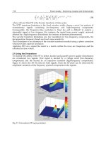
Fig. 11. Several modules are coupled to integrate the initial GEMPA architecture which offer
interesting functionalities; visualization 3-D environments as well as animation of motion
planning algorithms.

5.2 Recovering Objects Representation
People focus to solve problems using computer graphics, virtual reality and simulation of
motion planning techniques used to recover information related to objects inside the
environment through files which can storage information about triangle meshes. Hence,
several objects can be placed on different positions and orientations to simulate a three-
dimensional environment. There exist different formats to represent objects in three-
dimensional spaces (3-D), however, two conventions used for many tools to represent
triangle meshes are the most popular; objects based on off - files and objects based on txt -
files. In motion planning community there exist benchmarks represented through this kind
of files. GEMPA is able to load the triangle meshes used to represent objects from txt or off –
files. On the other hand, GEMPA allows the user to built news environments using
predefined figures as spheres, cones, cubes, etc. These figures are chosen from a option
menu and the user build environments using translation, rotation and scale transformations.
Each module on GEMPA architecture is presented in Figure 11 There, we can see that
initially, the main goal is the visualization of 3-D environments and the animation of motion
planning algorithms. In the case of visualization of 3-D environments, information is
recovered form files and the user can navigate through the environment using mouse and
keyboard controls. In the second case, the animation of motion planning algorithms,
GEMPA needs information about the problem. This problem is described by two elements;
the first one is called workspace, where obstacles (objects), robot representation and

configuration (position and orientation) is recovered from files; the second, a set of free
RobotLocalizationandMapBuilding170

collision configuration conform a path, this will be used to animate the robot movement
from initial to goal configuration. An example of 2D environment can be seen in Figure 12.













Fig. 12. Two different views of two-dimensional environment since the X-Y plane are
painted.

5.3 GUI and Navigation Tools
GEMPA has incorporated two modes to paint an object; wire mode and solid mode. Next,
Lambert illumination is implemented to produce more realism, and finally transparency
effects are used to visualize the objects. Along the GUI, camera movements are added to
facilitate the navigation inside the environment to display views from different locations. In
Figure 13. Two illumination techniques are presented when GEMPA recover information
since off-files to represent a human face.

Fig. 13. Light transparency. In the left side, an object is painted using Lambert illumination,
in the right side, transparency effect is applied on the object. Both features are used to give
more realism the environment.


5.4 Simulation of Motion Planning Algorithms
Initially, only PRM for free flying objects are considered as an initial application of GEMPA.
Taking into account this assumption, the workspace is conformed by a set of obstacles
(objects) distributed on the environment, these objects has movement restrictions that mean
that, the obstacles can not change their position inside the environment. In addition, an
object that can move through the workspace is added to the environment and is called
robot. The robot can move through the workspace using the free collision path to move from
the initial configuration to the goal configuration. For PRM for free flying objects, only a
robot can be defined and the workspace can include any obstacles as the problem need.
GEMPA also includes the capability to recover from an environment – file information about
the position and orientation for each object inside a workspace including the robot
configuration. Hence, GEMPA can draw each element to simulate the workspace associated.

Therefore, initially GEMPA can recover information about the workspace, an example of
this file can be see in Figure 14, where the environment file (left side), include initial and
goal configuration for the robot, beside includes x,y,z parameter for position and (α, β, γ)
parameters for orientation for every objects inside the workspace. Along with this
environment file, a configuration - file can also be loaded to generate the corresponding
animation of the free collision path. This configuration - file has the form presented in Figure
14 (right side). This file is conformed by n six-tuples (x, y, z,α, β, γ) to represent each
configuration included in the free collision path.

Fig. 14. On the left side, an example of environment - file (robot and obstacles representations)
is presented, and on the right side a configuration file (free collision path) is shown.

Once GEMPA has recovered information about workspace and collision free path, the tool
allows the user to display the animation on three different modes.

Mode 1: Animation painting all configurations.
Mode 2: Animation painting configurations using a step control.
Mode 3: Animation using automatic step.

From Figures 15 to Figure 18, we can see four different samples of motion planning
problems which are considered as important cases. For each one, different views are
KeyElementsforMotionPlanningAlgorithms 171

collision configuration conform a path, this will be used to animate the robot movement
from initial to goal configuration. An example of 2D environment can be seen in Figure 12.

Fig. 12. Two different views of two-dimensional environment since the X-Y plane are
painted.

5.3 GUI and Navigation Tools
GEMPA has incorporated two modes to paint an object; wire mode and solid mode. Next,
Lambert illumination is implemented to produce more realism, and finally transparency
effects are used to visualize the objects. Along the GUI, camera movements are added to
facilitate the navigation inside the environment to display views from different locations. In
Figure 13. Two illumination techniques are presented when GEMPA recover information
since off-files to represent a human face.

Fig. 13. Light transparency. In the left side, an object is painted using Lambert illumination,
in the right side, transparency effect is applied on the object. Both features are used to give
more realism the environment.


5.4 Simulation of Motion Planning Algorithms
Initially, only PRM for free flying objects are considered as an initial application of GEMPA.
Taking into account this assumption, the workspace is conformed by a set of obstacles
(objects) distributed on the environment, these objects has movement restrictions that mean
that, the obstacles can not change their position inside the environment. In addition, an
object that can move through the workspace is added to the environment and is called
robot. The robot can move through the workspace using the free collision path to move from
the initial configuration to the goal configuration. For PRM for free flying objects, only a
robot can be defined and the workspace can include any obstacles as the problem need.
GEMPA also includes the capability to recover from an environment – file information about
the position and orientation for each object inside a workspace including the robot
configuration. Hence, GEMPA can draw each element to simulate the workspace associated.
Therefore, initially GEMPA can recover information about the workspace, an example of
this file can be see in Figure 14, where the environment file (left side), include initial and
goal configuration for the robot, beside includes x,y,z parameter for position and (α, β, γ)
parameters for orientation for every objects inside the workspace. Along with this
environment file, a configuration - file can also be loaded to generate the corresponding
animation of the free collision path. This configuration - file has the form presented in Figure
14 (right side). This file is conformed by n six-tuples (x, y, z,α, β, γ) to represent each
configuration included in the free collision path.

Fig. 14. On the left side, an example of environment - file (robot and obstacles representations)

is presented, and on the right side a configuration file (free collision path) is shown.

Once GEMPA has recovered information about workspace and collision free path, the tool
allows the user to display the animation on three different modes.

Mode 1: Animation painting all configurations.
Mode 2: Animation painting configurations using a step control.
Mode 3: Animation using automatic step.

From Figures 15 to Figure 18, we can see four different samples of motion planning
problems which are considered as important cases. For each one, different views are
RobotLocalizationandMapBuilding172

presented to show GEMPA’s functionalities. Besides, we have presented motion planning
problems with different levels of complexity.
In Figure 15. (Sample 1) The collision free path is painted as complete option and as
animation option. In this sample a tetrahedron is considered as the robot.
Next, Figure 16: (Sample 2). A cube is presented as the robot for this motion planning
problem. Here, GEMPA presents the flat and wire modes to paint the objects.
In Figure 17: (Sample 3). Presents a robot which has a more complex for and the problem
becomes difficult to solve because the motion planning method needs to compute free
configuration in the narrow corridor.
Finally in Figure 18: (Sample 4). Animation painting all configurations (left side), and
animation using automatic step (right side) are displayed. Although the robot has not a
more complex form, there are various narrow corridors inside the environment.

Fig. 15. Sample 1. The robot is presented as a tetrahedron.

Fig. 16. Sample 2. The robot is presented as a cube.


Fig. 17. Sample 3. The robot’s form is more complex.











Fig. 18. Sample 4. More complex environment where various narrow corridors are presented.

6. References
Amato, N.; Bayazit, B. ; Dale, L.; Jones, C. &. Vallejo, D. (1998). Choosing good distance
metrics and local planer for probabilistic roadmap methods. In in Procc.IEEE Int.
Conf. Robot. Autom. (ICRA), pages 630–637.
Amato, N.; Bayazit, B. ; Dale, L.; Jones, C. &. Vallejo, D. (1998). Obprm: An obstaclebased
prm for 3d workspaces. In in Procc. Int. Workshop on Algorithmic Fundation of
Robotics (WAFR), pages 155–168.
Amato, N. M. & Wu, Y. (1996). A randomized roadmap method for path and manipulation
planning. In In IEEE Int. Conf. Robot. and Autom., pages 113–120.
Amato, N. Motion ning puzzels benchmarks.
Benitez, A. & Mugarte, A. (2009). GEMPA:Graphic Environment for Motion Planning
Algorithm. In Research in Computer Science, Advances in Computer Science and
Engineering. Volumen 42.
Benitez, A. & Vallejo, D. (2004). New Technique to Improve Probabilistic Roadmap Methods. In
proceedings of Mexican International Conference on Artificial Intelligence.
(IBERAMIA) Puebla City, November 22-26, pag. 514-526.
KeyElementsforMotionPlanningAlgorithms 173

presented to show GEMPA’s functionalities. Besides, we have presented motion planning
problems with different levels of complexity.
In Figure 15. (Sample 1) The collision free path is painted as complete option and as
animation option. In this sample a tetrahedron is considered as the robot.
Next, Figure 16: (Sample 2). A cube is presented as the robot for this motion planning
problem. Here, GEMPA presents the flat and wire modes to paint the objects.
In Figure 17: (Sample 3). Presents a robot which has a more complex for and the problem
becomes difficult to solve because the motion planning method needs to compute free
configuration in the narrow corridor.
Finally in Figure 18: (Sample 4). Animation painting all configurations (left side), and
animation using automatic step (right side) are displayed. Although the robot has not a
more complex form, there are various narrow corridors inside the environment.

Fig. 15. Sample 1. The robot is presented as a tetrahedron.

Fig. 16. Sample 2. The robot is presented as a cube.


Fig. 17. Sample 3. The robot’s form is more complex.

Fig. 18. Sample 4. More complex environment where various narrow corridors are presented.

6. References
Amato, N.; Bayazit, B. ; Dale, L.; Jones, C. &. Vallejo, D. (1998). Choosing good distance
metrics and local planer for probabilistic roadmap methods. In in Procc.IEEE Int.
Conf. Robot. Autom. (ICRA), pages 630–637.
Amato, N.; Bayazit, B. ; Dale, L.; Jones, C. &. Vallejo, D. (1998). Obprm: An obstaclebased
prm for 3d workspaces. In in Procc. Int. Workshop on Algorithmic Fundation of
Robotics (WAFR), pages 155–168.
Amato, N. M. & Wu, Y. (1996). A randomized roadmap method for path and manipulation
planning. In In IEEE Int. Conf. Robot. and Autom., pages 113–120.
Amato, N. Motion ning puzzels benchmarks.
Benitez, A. & Mugarte, A. (2009). GEMPA:Graphic Environment for Motion Planning
Algorithm. In Research in Computer Science, Advances in Computer Science and
Engineering. Volumen 42.
Benitez, A. & Vallejo, D. (2004). New Technique to Improve Probabilistic Roadmap Methods. In
proceedings of Mexican International Conference on Artificial Intelligence.
(IBERAMIA) Puebla City, November 22-26, pag. 514-526.
RobotLocalizationandMapBuilding174

Benitez, A.; Vallejo, D. & Medina, M.A. (2004). Prms based on obstacle’s geometry.In In
Proc. IEEE The 8th Conference on Intelligent Autonomous Systems, pages 592–599.
Boor, V.; Overmars, N. H. & van der Stappen, A. F. (1999). The gaussian sampling strategy
for probabilistic roadmap planners. In In IEEE Int. Conf. Robot. And Autom., pages
1018–1023.
Chang, H. & Li, T. Y. (1995). Assembly maintainability study with motion planning. In In
Proc. IEEE Int. Conf. on Rob. and Autom., pages 1012–1019.

Christoph, M. Hoffmann. Solid modeling. (1997). In Handbook of Discrete and
ComputationalGeometry, pages 863,880. In Jacob E. Goodman and Joseph
ORourke, editors Press, Boca Raton New York.
Goodman, J. & O’Rourke, J. (1997). Handbook of Discrete and Computational Geometry.
CRC Press.In Computer Graphics (SIGGRAPH’94)., pages 395–408.
Kavraki, L. & Latombe, J.C. (1994). Randomized preprocessing of configuration space for
path planning. In IEEE Int. Conf. Robot. and Autom, pages 2138–2145.
Kavraki, L. & Latombe, J.C. (1994). Randomized preprocessing of configuration space for
fast path planning. In IEEE International Conference on Robotics and Automation,
San Diego (USA), pp. 2138-2245.
Kavraki, L. E.; Svestka, P.; Latombe, J C. & Overmars, M. H. (1996). Probabilistic roadmaps
for path planning in high-dimensional configuration spaces. In IEEE Trans. Robot.
& Autom, pages 566–580 .
Kavraki, L.; Kolountzakis, L. & Latombe, JC. (1996). Analysis of probabilistic roadmaps for
path planning. In IEEE International Conference on Robotics and Automation,
Minneapolis (USA), pp. 3020-3025.
Kavraki, L.E, J.C. Latombe, R. Motwani, & P. Raghavan. (1995). Randomized preprocessing
of configuration space for path planning. In Proc. ACM Symp. on Theory of
Computing., pages 353–362.
Koga, Y.; Kondo, K.; Kuffner, J. & Latombe, J.C. (1994). Planning motions with intentions.
Latombe, J.C. (1991). Robot Motion Planning. Kluwer Academic Publishers, Boston, MA.
Laumond, J. P. & Siméon, T. (2000). Notes on visibility roadmaps and path planning. In In
Proc. Int. Workshop on Algorithmic Foundation of Robotics (WAFR), pages67–77.
M. LaValle and J. J. Kuffner. (1999). Randomized kinodynamic planning. In IEEE Int. Conf.
Robot. and Autom. (ICRA), pages 473–479.
M. LaValle, J.H. Jakey, and L.E. Kavraki. (1999). A probabilistic roadmap approach for
systems with closed kinematic chains. In IEEE Int. Conf. Robot. and Autom.
Overmars, M. & Svestka, P. (1995). A Probabilistic learning approach to motion Planning.
In Algorithmic Foundations of Robotics of (WAFR94), K. Goldberg et al (Eds), pp.
19-37, AK Peters.

Overmars, M. & Svestka, P. (1994). A probabilistic learning approach to motion planning. In
Proc. Workshop on Algorithmic Foundations of Robotics., pages 19–37.
Russell, S. & Norvig, P. (2003). Articial Intelligence: A Modern Approach. Pearson
Education, Inc., Upper Saddle River, NJ.
Steven, M. LaValle. (2004). Planning Algorithms.
Tombropoulos, R.Z.; Adler, J.R. & Latombe, J.C. Carabeamer. (1999). A treatment planner
for a robotic radiosurgical system with general kinematics. In Medical Image
Analysis, pages 237–264.

OptimumBipedTrajectoryPlanningforHumanoidRobotNavigationinUnseenEnvironment 175
OptimumBipedTrajectoryPlanningforHumanoidRobotNavigationin
UnseenEnvironment
HanaahYussofandMasahiroOhka
X

Optimum Biped Trajectory Planning for
Humanoid Robot Navigation in Unseen
Environment

Hanafiah Yussof
1,2
and Masahiro Ohka
1

1
Graduate School of Information Science, Nagoya University
Japan
2
Faculty of Mechanical Engineering, Universiti Teknologi MARA
Malaysia

1. Introduction

The study on biped locomotion in humanoid robots has gained great interest since the last
decades (Hirai et. al. 1998, Hirukawa et. al., 2004, Ishiguro, 2007). This interest are motivated
from the high level of mobility, and the high number of degrees of freedom allow this kind
of mobile robot adapt and move upon very unstructured sloped terrain. Eventually, it is
more desirable to have robots of human build instead of modifying environment for robots
(Khatib et. al, 1999). Therefore, a suitable navigation system is necessary to guide the robot’s
locomotion during real-time operation. In fundamental robot navigation studies, robot
system is normally provided with a map or a specific geometrical guidance to complete its
tasks (Okada et al., 2003, Liu et al., 2002). However during operation in uncertain
environment such as in emergency sites like an earthquake site, or even in a room that the
robots never been there before, which is eventually become the first experience for them,
robots needs some intelligence to recognize and estimate the position and structure of
objects around them. The most important is robot must localize its position within this
environment and decide suitable action based on the environment conditions. To archives
its target tasks, the robot required a highly reliable sensory devices for vision, scanning, and
touching to recognize surrounding. These problems have become the main concern in our
research that deals with humanoid robot for application in built-for-human environment.
Operation in unseen environment or areas where visual information is very limited is a new
challenge in robot navigation. So far there was no much achievement to solve robot
navigation in such environments. In previous research, we have proposed a contact
interaction-based navigation strategy in a biped humanoid robot to operate in unseen
environment (Hanafiah et al., 2008). In this chapter, we present analysis results of optimum
biped trajectory planning for humanoid robot navigation to minimize possibility of collision
during operation in unseen environment. In this analysis, we utilized 21-dof biped
humanoid robot Bonten-Maru II. Our aim is to develop reliable walking locomotion in order
9
RobotLocalizationandMapBuilding176

to support the main tasks in the humanoid robot navigation system. Fig. 1 shows diagram of
humanoid robot Bonten-Maru II and its configurations of dofs.


Fig. 1. Humanoid Robot Bonten-Maru II and its configuration of dofs.

It is inevitable that stable walking gait strategy is required to provide efficient and reliable
locomotion for biped robots. In the biped locomotion towards application in unseen
environment, we identified three basic motions: walk forward and backward directions,
side-step to left and right, and yawing movement to change robot’s orientation. In this
chapter, at first we analyzed the joint trajectory generation in humanoid robot legs to define
efficient gait pattern. We present kinematical solutions and optimum gait trajectory patterns
for humanoid robot legs. Next, we performed analysis to define efficient walking gait
locomotion by improvement of walking speed and travel distance without reducing
reduction-ratio at joint-motor system. This is because sufficient reduction-ratio is required
by the motor systems to supply high torque to the robot’s manipulator during performing
tasks such as object manipulation and obstacle avoidance. We also present optimum yawing
motion strategy for humanoid robot to change its orientation within confined space. The
analysis results were verified with simulation and real-time experiment with humanoid
robot Bonten-Maru II.
Eventually, to safely and effectively navigate robots in unseen environment, the navigation
system must feature reliable collision checking method to avoid collisions. In this chapter,
we present analyses of collision checking using the robot arms to perform searching,
touching and grasping motions in order to recognize its surrounding condition. The
collision checking is performed in searching motion of the robot’s arms that created a radius
of detection area within the arm’s reach. Based on the searching area coverage of the robot
arms, we geometrically analyze the robot biped motions using Rapid-2D CAD software to
identify the ideal collision free area. The collision free area is used to calculate maximum
biped step-length when no object is detected. Consequently the robot control system created

an absolute collision free area for the robot to generate optimum biped trajectories. In case of
object is detected during searching motion, the robot arm will touch and grasp the object
surface to define self-localization, and consequently optimum step-length is refined.
Z

Y
X
Yaw

R
oll
P
itch


Verification experiments were conducted using humanoid robot Bonten-Maru II to operate
in a room with walls and obstacles was conducted. In this experiment, the robot visual
sensors are not connected to the system. Therefore the robot locomotion can only rely on
contact interaction of the arms that are equipped with force sensors.

2. Short Survey on Humanoid Robot Navigation

Operation in unseen environment or areas where visual information is very limited is a new
challenge in robot navigation. So far there was no much achievement to solve robot
navigation in such environments. In normal conditions, it is obvious that a navigation
system that applies non-contact sensors such as vision sensors provides intensive
information about the environment (Sagues & Guerrero, 1999). However, robots cannot just
rely on this type of sensing information to effectively work and cooperate with humans. For
instance, in real applications the robots are likely to be required to operate in areas where
vision information is very limited, such as in a dark room or during a rescue mission at an

earthquake site (Diaz et. al., 2001). Moreover vision sensors have significant measurement
accuracy problems resulting from technical problems such as low camera resolution and the
dependence of stereo algorithms on specific image characteristics. Furthermore, the cameras
are normally located at considerable distance from objects in the environment where
operation takes place, resulting in approximate information of the environment.
In addition to the above, a laser range finder has also been applied in a robot navigation
system (Thompson et. al., 2006). This sensor is capable of producing precise distance
information and provides more accurate measurements compared with the vision sensor.
However, it is impractical to embed this type of sensor with its vision analysis system in a
walking robot system because of its size and weight (Okada et. al., 2003). A navigation
system that applies contact-based sensors is capable of solving the above problems,
particularly for a biped walking robot system (Hanafiah et. al., 2007). This type of sensor can
accurately gauge the structure of the environment, thus making it suitable to support
current navigation systems that utilize non-contact sensors. Furthermore, the system
architecture is simpler and can easily be mounted on the walking robot body.
Eventually, to safely and effectively navigate robots in unseen environment, the navigation
system must feature reliable collision checking method to avoid collisions. To date, in
collision checking and prediction research, several methods such as vision based local floor
map (Okada et al., 2003, Liu et al., 2002) and cylinder model (Guttmann et al., 2005) have
been proposed for efficient collision checking and obstacle recognition in biped walking
robot. In addition, Kuffner (Kuffner et al., 2002) have used fast distance determination
method for self-collision detection and prevention for humanoid robots. This method is for
convex polyhedra in order to conservatively guarantee that the given trajectory is free of
self-collision. However, to effectively detect objects based on contact-based sensors, such
methods are not suitable because they are mostly based on assumption of environment
conditions acquired by non-contact sensors such as vision and laser range sensors.
Several achievements have been reported related with navigation in humanoid robots.
Ogata have proposed human-robot collaboration based on quasi-symbolic expressions
applying humanoid on static platform named Robovie (Ogata et al., 2005). This work
combined non-contact and contact sensing approach in collaboration of human and robot

during navigation tasks. This is the closest work with the approach used in this research.
OptimumBipedTrajectoryPlanningforHumanoidRobotNavigationinUnseenEnvironment 177

to support the main tasks in the humanoid robot navigation system. Fig. 1 shows diagram of
humanoid robot Bonten-Maru II and its configurations of dofs.


Fig. 1. Humanoid Robot Bonten-Maru II and its configuration of dofs.

It is inevitable that stable walking gait strategy is required to provide efficient and reliable
locomotion for biped robots. In the biped locomotion towards application in unseen
environment, we identified three basic motions: walk forward and backward directions,
side-step to left and right, and yawing movement to change robot’s orientation. In this
chapter, at first we analyzed the joint trajectory generation in humanoid robot legs to define
efficient gait pattern. We present kinematical solutions and optimum gait trajectory patterns
for humanoid robot legs. Next, we performed analysis to define efficient walking gait
locomotion by improvement of walking speed and travel distance without reducing
reduction-ratio at joint-motor system. This is because sufficient reduction-ratio is required
by the motor systems to supply high torque to the robot’s manipulator during performing
tasks such as object manipulation and obstacle avoidance. We also present optimum yawing
motion strategy for humanoid robot to change its orientation within confined space. The
analysis results were verified with simulation and real-time experiment with humanoid
robot Bonten-Maru II.
Eventually, to safely and effectively navigate robots in unseen environment, the navigation
system must feature reliable collision checking method to avoid collisions. In this chapter,
we present analyses of collision checking using the robot arms to perform searching,
touching and grasping motions in order to recognize its surrounding condition. The
collision checking is performed in searching motion of the robot’s arms that created a radius
of detection area within the arm’s reach. Based on the searching area coverage of the robot
arms, we geometrically analyze the robot biped motions using Rapid-2D CAD software to

identify the ideal collision free area. The collision free area is used to calculate maximum
biped step-length when no object is detected. Consequently the robot control system created
an absolute collision free area for the robot to generate optimum biped trajectories. In case of
object is detected during searching motion, the robot arm will touch and grasp the object
surface to define self-localization, and consequently optimum step-length is refined.
Z

Y
X
Yaw

R
oll
P
itch


Verification experiments were conducted using humanoid robot Bonten-Maru II to operate
in a room with walls and obstacles was conducted. In this experiment, the robot visual
sensors are not connected to the system. Therefore the robot locomotion can only rely on
contact interaction of the arms that are equipped with force sensors.

2. Short Survey on Humanoid Robot Navigation

Operation in unseen environment or areas where visual information is very limited is a new
challenge in robot navigation. So far there was no much achievement to solve robot
navigation in such environments. In normal conditions, it is obvious that a navigation
system that applies non-contact sensors such as vision sensors provides intensive
information about the environment (Sagues & Guerrero, 1999). However, robots cannot just
rely on this type of sensing information to effectively work and cooperate with humans. For

instance, in real applications the robots are likely to be required to operate in areas where
vision information is very limited, such as in a dark room or during a rescue mission at an
earthquake site (Diaz et. al., 2001). Moreover vision sensors have significant measurement
accuracy problems resulting from technical problems such as low camera resolution and the
dependence of stereo algorithms on specific image characteristics. Furthermore, the cameras
are normally located at considerable distance from objects in the environment where
operation takes place, resulting in approximate information of the environment.
In addition to the above, a laser range finder has also been applied in a robot navigation
system (Thompson et. al., 2006). This sensor is capable of producing precise distance
information and provides more accurate measurements compared with the vision sensor.
However, it is impractical to embed this type of sensor with its vision analysis system in a
walking robot system because of its size and weight (Okada et. al., 2003). A navigation
system that applies contact-based sensors is capable of solving the above problems,
particularly for a biped walking robot system (Hanafiah et. al., 2007). This type of sensor can
accurately gauge the structure of the environment, thus making it suitable to support
current navigation systems that utilize non-contact sensors. Furthermore, the system
architecture is simpler and can easily be mounted on the walking robot body.
Eventually, to safely and effectively navigate robots in unseen environment, the navigation
system must feature reliable collision checking method to avoid collisions. To date, in
collision checking and prediction research, several methods such as vision based local floor
map (Okada et al., 2003, Liu et al., 2002) and cylinder model (Guttmann et al., 2005) have
been proposed for efficient collision checking and obstacle recognition in biped walking
robot. In addition, Kuffner (Kuffner et al., 2002) have used fast distance determination
method for self-collision detection and prevention for humanoid robots. This method is for
convex polyhedra in order to conservatively guarantee that the given trajectory is free of
self-collision. However, to effectively detect objects based on contact-based sensors, such
methods are not suitable because they are mostly based on assumption of environment
conditions acquired by non-contact sensors such as vision and laser range sensors.
Several achievements have been reported related with navigation in humanoid robots.
Ogata have proposed human-robot collaboration based on quasi-symbolic expressions

applying humanoid on static platform named Robovie (Ogata et al., 2005). This work
combined non-contact and contact sensing approach in collaboration of human and robot
during navigation tasks. This is the closest work with the approach used in this research.
RobotLocalizationandMapBuilding178

However Ogata use humanoid robot without leg. On the other hand, related with biped
humanoid robot navigation, the most interesting work was presented by Stasse where visual
3D Simultaneous Localization and Mapping (SLAM) was used to navigate HRP-2 humanoid
robot performing visual loop-closing motion (Stasse et al., 2006). In other achievements,
Gutmann (Gutmann et al., 2005) have proposed real-time path planning for humanoid robot
navigation. The work was evaluated using QRIO Sony’s small humanoid robot equipped
with stereo camera. Meanwhile, Seara have evaluated methodological aspects of a scheme
for visually guided humanoid robot navigation using simulation (Seara et al., 2004). Next,
Okada have proposed humanoid robot navigation system using vision based local floor
map (Okada et al., 2003). Related with sensory-based biped walking, Ogura (Ogura et al.,
2004) has proposed a sensory-based biped walking motion instruction strategy for
humanoid robot using visual and auditory sensors to generate walking patterns according
to human orders and to memorize various complete walking patterns. In previous research,
we have proposed a contact interaction-based navigation strategy in a biped humanoid
robot to operate in unseen environment (Hanafiah et. al., 2008). In this chapter, we present
analysis results of optimum biped trajectory planning for humanoid robot navigation to
minimize possibility of collision during operation in unseen environment.

3. Simplification of Kinematics Solutions

A reliable trajectory generation formulations will directly influence stabilization of robot
motion especially during operation in unseen environment where the possibility of unstable
biped walking due to ground condition and collision with unidentified objects are rather
high if compared to operation in normal condition. In this chapter, at first we analyzed the
joint trajectory generation in humanoid robot legs to define efficient gait pattern. We present

kinematical solutions and optimum gait trajectory patterns for humanoid robot legs.
Eventually, formulations to generate optimum trajectory in articulated joints and
manipulators are inevitable in any types of robots, especially for legged robot. Indeed, the
most sophisticated forms of legged motion are that of biped gait locomotion. However
calculation to solve kinematics problems to generate trajectory for robotic joints is a
complicated and time-consuming study, especially when it involves a complex joint
structure. Furthermore, computation of joint variables is also needed to compute the
required joint torques for the actuators. In current research, to generate optimum robot
trajectory, we simplified kinematics formulation to generate trajectory for each robot joint in
order to reduce calculation time and increase reliability of robot arms and legs motions. This
is necessary because during operation in unseen environment, robot will mainly rely on
contact interaction using its arms. Consequently, an accurate and fast respond of robot’s
both legs are very important to maintain stability of its locomotion.
We implemented a simplified approach to solving inverse kinematics problems by
classifying the robot’s joints into several groups of joint coordinate frames at the robot’s
manipulator. To describe translation and rotational relationship between adjacent joint
links, we employ a matrix method proposed by Denavit-Hartenberg (Denavit & Hartenberg,
1955), which systematically establishes a coordinate system for each link of an articulated
chain. Since this chapter focusing on biped trajectory, we present kinematical analysis of 6-
dofs leg in the humanoid robot Bonten-Maru II body.

3.1 Kinematical Solutions of 6-DOFs Leg
Each of the legs has six dofs: three dofs (yaw, roll and pitch) at the hip joint, one dof (pitch)
at the knee joint and two dofs (pitch and roll) at the ankle joint. In this research, we solve
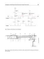
only inverse kinematics calculations for the robot leg. Figure 2 shows the structure and
configuration of joints and links in the robot’s leg. A reference coordinate is taken at the
intersection point of the 3-dofs hip joint.


o

x
1
, zz
o
1
x
2
z
3
z
3
x
4
x
4
z
5
z
5
x
6
z
6
x
h
x
h
z
h
y

o
y
o
x
1
, zz
o
1
x
2
z
3
z
3
x
4
x
4
z
5
z
5
x
6
z
6
x
h
x
h

z
h
y
o
y

Fig. 2. Leg structure of Bonten-Maru II and configurations of joint coordinates.

Link θ
ileg

d


l
0
θ
1leg
+90º
0 0 0
1
θ
2leg
-90 º
0 90 º 0
2
θ
3leg

0 90 º 0

3
θ
4leg

0 0 l
1

4
θ
5leg

0 0 l
2

5
θ
6leg

0 -90 º 0
6 0 0 0 l
3

Table 1. Link parameters of the 6-dofs humanoid robot leg.

In solving calculations of inverse kinematics for the leg, the joint coordinates are divided
into eight separate coordinate frames as listed bellow:

0
： Reference coordinate.


1
： Hip yaw coordinate.

2
： Hip roll coordinate.

3
： Hip pitch coordinate.

4
： Knee pitch coordinate.

5
： Ankle pitch coordinate.

6
： Ankle roll coordinate.

h
： Foot bottom-center coordinate.
OptimumBipedTrajectoryPlanningforHumanoidRobotNavigationinUnseenEnvironment 179

However Ogata use humanoid robot without leg. On the other hand, related with biped
humanoid robot navigation, the most interesting work was presented by Stasse where visual
3D Simultaneous Localization and Mapping (SLAM) was used to navigate HRP-2 humanoid
robot performing visual loop-closing motion (Stasse et al., 2006). In other achievements,
Gutmann (Gutmann et al., 2005) have proposed real-time path planning for humanoid robot
navigation. The work was evaluated using QRIO Sony’s small humanoid robot equipped
with stereo camera. Meanwhile, Seara have evaluated methodological aspects of a scheme
for visually guided humanoid robot navigation using simulation (Seara et al., 2004). Next,

Okada have proposed humanoid robot navigation system using vision based local floor
map (Okada et al., 2003). Related with sensory-based biped walking, Ogura (Ogura et al.,
2004) has proposed a sensory-based biped walking motion instruction strategy for
humanoid robot using visual and auditory sensors to generate walking patterns according
to human orders and to memorize various complete walking patterns. In previous research,
we have proposed a contact interaction-based navigation strategy in a biped humanoid
robot to operate in unseen environment (Hanafiah et. al., 2008). In this chapter, we present
analysis results of optimum biped trajectory planning for humanoid robot navigation to
minimize possibility of collision during operation in unseen environment.

3. Simplification of Kinematics Solutions

A reliable trajectory generation formulations will directly influence stabilization of robot
motion especially during operation in unseen environment where the possibility of unstable
biped walking due to ground condition and collision with unidentified objects are rather
high if compared to operation in normal condition. In this chapter, at first we analyzed the
joint trajectory generation in humanoid robot legs to define efficient gait pattern. We present
kinematical solutions and optimum gait trajectory patterns for humanoid robot legs.
Eventually, formulations to generate optimum trajectory in articulated joints and
manipulators are inevitable in any types of robots, especially for legged robot. Indeed, the
most sophisticated forms of legged motion are that of biped gait locomotion. However
calculation to solve kinematics problems to generate trajectory for robotic joints is a
complicated and time-consuming study, especially when it involves a complex joint
structure. Furthermore, computation of joint variables is also needed to compute the
required joint torques for the actuators. In current research, to generate optimum robot
trajectory, we simplified kinematics formulation to generate trajectory for each robot joint in
order to reduce calculation time and increase reliability of robot arms and legs motions. This
is necessary because during operation in unseen environment, robot will mainly rely on
contact interaction using its arms. Consequently, an accurate and fast respond of robot’s
both legs are very important to maintain stability of its locomotion.

We implemented a simplified approach to solving inverse kinematics problems by
classifying the robot’s joints into several groups of joint coordinate frames at the robot’s
manipulator. To describe translation and rotational relationship between adjacent joint
links, we employ a matrix method proposed by Denavit-Hartenberg (Denavit & Hartenberg,
1955), which systematically establishes a coordinate system for each link of an articulated
chain. Since this chapter focusing on biped trajectory, we present kinematical analysis of 6-
dofs leg in the humanoid robot Bonten-Maru II body.

3.1 Kinematical Solutions of 6-DOFs Leg
Each of the legs has six dofs: three dofs (yaw, roll and pitch) at the hip joint, one dof (pitch)
at the knee joint and two dofs (pitch and roll) at the ankle joint. In this research, we solve
only inverse kinematics calculations for the robot leg. Figure 2 shows the structure and
configuration of joints and links in the robot’s leg. A reference coordinate is taken at the
intersection point of the 3-dofs hip joint.


o
x
1
, zz
o
1
x
2
z
3
z
3
x
4

x
4
z
5
z
5
x
6
z
6
x
h
x
h
z
h
y
o
y
o
x
1
, zz
o
1
x
2
z
3
z

3
x
4
x
4
z
5
z
5
x
6
z
6
x
h
x
h
z
h
y
o
y

Fig. 2. Leg structure of Bonten-Maru II and configurations of joint coordinates.

Link θ
ileg

d


l
0
θ
1leg
+90º
0 0 0
1
θ
2leg
-90 º
0 90 º 0
2
θ
3leg

0 90 º 0
3
θ
4leg

0 0 l
1

4
θ
5leg

0 0 l
2

5
θ
6leg

0 -90 º 0
6 0 0 0 l
3

Table 1. Link parameters of the 6-dofs humanoid robot leg.

In solving calculations of inverse kinematics for the leg, the joint coordinates are divided
into eight separate coordinate frames as listed bellow:

0
： Reference coordinate.

1
： Hip yaw coordinate.

2
： Hip roll coordinate.

3
： Hip pitch coordinate.

4
： Knee pitch coordinate.

5

： Ankle pitch coordinate.

6
： Ankle roll coordinate.

h
： Foot bottom-center coordinate.
RobotLocalizationandMapBuilding180

Figure 2 also shows a model of the robot leg that indicates the configurations and
orientation of each set of joint coordinates. Here, link length for the thigh is l
1
, while for the
shin it is l
2
. Link parameters for the leg are defined in Table 1. From the Denavit-Hartenberg
convention mentioned above, definitions of the homogeneous transform matrix of the link
parameters can be described as follows:
0
h
T= Rot(z
i
,θ
i
)Trans(0,0,d
i
)Trans(l
i
,0,0)Rot(x
i

,

i
). (1)
Here, variable factor θ
i
is the joint angle between the x
i-1
and the x
i
-axes measured about the
z
i
axis; d
i
is the distance from the x
i-1
axis to the x
i
axis measured along the z
i
axis;

i
is the
angle between the z
i
axis to the z
i-1
axis measured about the x

i-1
axis, and l
i
is the distance
from the z
i
axis to the z
i-1
axis measured along the x
i-1
axis. Referring to Fig. 2, the
transformation matrix at the bottom of the foot (
6
h
T) is an independent link parameter
because the coordinate direction is changeable. Here, to simplify the calculations, the ankle
joint is positioned so that the bottom of the foot settles on the floor surface. The leg’s
orientation is fixed from the reference coordinate so that the third row of the rotation matrix
at the leg’s end becomes like equation (2).
 
T
zleg
P 100 (2)
Furthermore, the leg’s links are classified into three groups to short-cut the calculations,
where each group of links is calculated separately as follows:
i) From link 0 to link 1 (Reference coordinate to coordinate joint number 1).
ii) From link 1 to link 4 (Coordinate joint no. 2 to coordinate joint no. 4).
iii) From link 4 to link 6 (Coordinate joint no. 5 to coordinate at the bottom of the foot).
Basically, i) is to control leg rotation at the z-axis, ii) is to define the leg position, while iii) is
to decide the leg’s end-point orientation. A coordinate transformation matrix can be

arranged as following.
0
h
T=
0
1
T
1
4
T
4
h
T= (
0
h
T)(
1
2
T
2
3
T
3
4
T)(
4
5
T
5
6

T
6
h
T) (3)
Here, the coordinate transformation matrices for
1
4
T and
4
h
T can be defined as (4) and (5),
respectively.
1
4
T=
1
2
T
2
3
T
3
4
T



















1000
0
3212342342
313434
3212342342
cclssccc
slcs
cslcsscs
(4)
4
h
T=
4
5
T
5
6
T

6
h
T


















1000
0
6366
65356565
653256565
slcs
cslcsscs
ccllssccc
(5)

The coordinate transformation matrix for
0
h
T, which describes the leg’s end-point position
and orientation, can be shown with the following equation.

0
h
T















1000
333231
232221
131211
z
y

x
prrr
prrr
prrr
(6)
From equation (2), the following conditions were satisfied.
10
3332312313





rrrrr ,
(7)
Hence, joint rotation angles θ
1leg
~θ
6leg
can be defined by applying the above conditions. First,
considering i), in order to provide rotation at the z-axis, only the hip joint needs to rotate in
the yaw direction, specifically by defining θ
1leg
. As mentioned earlier, the bottom of the foot
settles on the floor surface; therefore, the rotation matrix for the leg’s end-point measured
from the reference coordinate can be defined by the following equation.
0
h
R
),(Rot

leg
1

z
























100
0

0
100
0
0
2221
1211
11
11
rr
rr
cs
sc
legleg
legleg


(8)
Here, θ
1leg
can be defined as below.
 
22211
rr ,atan2
leg


(9)
Next, considering ii), from the obtained result of θ
1leg
,

0
h
T is defined in (9).
0
h
T

















1000
100
0
0
11
11
leg

leg
leg
z
y
x
P
Psc
Pcs
(10)
Here, from constrain orientation of the leg’s end point, the position vector of joint 5 is
defined as follows in (11), and its relative connection with the matrix is defined in (12). Next,
equation (13) is defined relatively.
0
P
5
=
0
4
T
4
P
5
T
zyx
lPPP








3
leg
leg
leg
, (11)
5
010
1
5
41
4
PTPT
ˆˆ


(12)

































































11000
0100
00
00
1
0
0
1000
0

3
11
112
3212342342
313434
3212342342
lp
p
p
sc
csl
cclssccc
slcs
cslcsscs
z
y
x
(13)
Therefore,
 
 
 





























342312
34231
342312
clclc
slcl
clcls
P
P
P
z

y
x
leg
leg
leg
ˆ
ˆ
ˆ
. (14)
OptimumBipedTrajectoryPlanningforHumanoidRobotNavigationinUnseenEnvironment 181

Figure 2 also shows a model of the robot leg that indicates the configurations and
orientation of each set of joint coordinates. Here, link length for the thigh is l
1
, while for the
shin it is l
2
. Link parameters for the leg are defined in Table 1. From the Denavit-Hartenberg
convention mentioned above, definitions of the homogeneous transform matrix of the link
parameters can be described as follows:
0
h
T= Rot(z
i
,θ
i
)Trans(0,0,d
i
)Trans(l
i

,0,0)Rot(x
i
,

i
). (1)
Here, variable factor θ
i
is the joint angle between the x
i-1
and the x
i
-axes measured about the
z
i
axis; d
i
is the distance from the x
i-1
axis to the x
i
axis measured along the z
i
axis;

i
is the
angle between the z
i
axis to the z

i-1
axis measured about the x
i-1
axis, and l
i
is the distance
from the z
i
axis to the z
i-1
axis measured along the x
i-1
axis. Referring to Fig. 2, the
transformation matrix at the bottom of the foot (
6
h
T) is an independent link parameter
because the coordinate direction is changeable. Here, to simplify the calculations, the ankle
joint is positioned so that the bottom of the foot settles on the floor surface. The leg’s
orientation is fixed from the reference coordinate so that the third row of the rotation matrix
at the leg’s end becomes like equation (2).


T
zleg
P 100 (2)
Furthermore, the leg’s links are classified into three groups to short-cut the calculations,
where each group of links is calculated separately as follows:
i) From link 0 to link 1 (Reference coordinate to coordinate joint number 1).
ii) From link 1 to link 4 (Coordinate joint no. 2 to coordinate joint no. 4).

iii) From link 4 to link 6 (Coordinate joint no. 5 to coordinate at the bottom of the foot).
Basically, i) is to control leg rotation at the z-axis, ii) is to define the leg position, while iii) is
to decide the leg’s end-point orientation. A coordinate transformation matrix can be
arranged as following.
0
h
T=
0
1
T
1
4
T
4
h
T= (
0
h
T)(
1
2
T
2
3
T
3
4
T)(
4
5

T
5
6
T
6
h
T) (3)
Here, the coordinate transformation matrices for
1
4
T and
4
h
T can be defined as (4) and (5),
respectively.
1
4
T=
1
2
T
2
3
T
3
4
T



















1000
0
3212342342
313434
3212342342
cclssccc
slcs
cslcsscs
(4)
4
h
T=
4
5
T

5
6
T
6
h
T


















1000
0
6366
65356565
653256565
slcs

cslcsscs
ccllssccc
(5)
The coordinate transformation matrix for
0
h
T, which describes the leg’s end-point position
and orientation, can be shown with the following equation.

0
h
T















1000
333231
232221

131211
z
y
x
prrr
prrr
prrr
(6)
From equation (2), the following conditions were satisfied.
10
3332312313
 rrrrr ,
(7)
Hence, joint rotation angles θ
1leg
~θ
6leg
can be defined by applying the above conditions. First,
considering i), in order to provide rotation at the z-axis, only the hip joint needs to rotate in
the yaw direction, specifically by defining θ
1leg
. As mentioned earlier, the bottom of the foot
settles on the floor surface; therefore, the rotation matrix for the leg’s end-point measured
from the reference coordinate can be defined by the following equation.
0
h
R
),(Rot
leg
1


z
























100
0
0
100

0
0
2221
1211
11
11
rr
rr
cs
sc
legleg
legleg


(8)
Here, θ
1leg
can be defined as below.
 
22211
rr ,atan2
leg


(9)
Next, considering ii), from the obtained result of θ
1leg
,
0
h

T is defined in (9).
0
h
T

















1000
100
0
0
11
11
leg
leg
leg

z
y
x
P
Psc
Pcs
(10)
Here, from constrain orientation of the leg’s end point, the position vector of joint 5 is
defined as follows in (11), and its relative connection with the matrix is defined in (12). Next,
equation (13) is defined relatively.
0
P
5
=
0
4
T
4
P
5
T
zyx
lPPP








3
leg
leg
leg
, (11)
5
010
1
5
41
4
PTPT
ˆˆ


(12)

































































11000
0100
00
00
1
0
0
1000
0
3
11

112
3212342342
313434
3212
342342
lp
p
p
sc
csl
cclssccc
slcs
cslcsscs
z
y
x
(13)
Therefore,
 
 
 





























342312
34231
342312
clclc
slcl
clcls
P
P
P
z
y

x
leg
leg
leg
ˆ
ˆ
ˆ
. (14)
RobotLocalizationandMapBuilding182

To define joint angles
θ
2leg
, θ
3leg
, θ
4leg
, equation (14) is used. Therefore, the rotation angles are
defined as the following equations:






 CC ,atan2
leg
2
4
1


(15)

 
213
kkpp
yxz
,atan2
ˆ
,
ˆ
atan2
leg
legleg









(16)



legleg
leg
ˆ

,
ˆ
atan2
zx
pp
2

. (17)

Eventually,
21xz
kkpC ,,
ˆ
,
leg
are defined as follows:
21
2
2
2
1
222
2 ll
llppp
C
zyx
)(
ˆˆˆ
leg
leg

leg


(18)

22
leglegleg
ˆˆˆ
zxxz
ppp 
(19)

4224211
slkcllk  ,
(20)
Finally, considering iii), joint angles θ
5leg
and

θ
6 leg
are defined geometrically by the following
equations:
leglegleg
435



 (21)
leg

leg
26


 . (22)

3.2 Interpolation and Gait Trajectory Pattern
A common way of making a robot’s manipulator to move from start point to end point in a
smooth, controlled fashion is to have each joint to move as specified by a smooth function of
time
t. Each joint starts and ends its motion at the same time, thus the robot’s motion
appears to be coordinated. In this research, we employ degree-5 polynomial equations to
solve interpolation from start point
P
0
to end point P
f
. Degree-5 polynomial equations
provides smoother gait trajectory compared to degree-3 polynomial equations which
commonly used in robotic control. Velocity and acceleration at
P
0
and P
f
are defined as zero;
only the position factor is considered as a coefficient for performing interpolation.
5
5
4
4

3
3
2
210
tatatatataatP )( (23)
Time factor at
P
0
and P
f
are describe as t
0
= 0 and t
f
, respectively. Here, boundary condition
for each position, velocity and acceleration at P
0
and P
f
are shown at following equations.





















fffff
ffffff
fffffff
o
o
o
PtatataatP
PtatatataatP
PtatatatataatP
PaP
PaP
PaP




3
5
2
432

4
5
3
4
2
321
5
5
4
4
3
3
2
210
2
1
0
201262
5432
20
0
0
)(
)(
)(
)(
)(
)(
(24)
Here, coefficient

a
i
(i = 0,1,2,3,4,5) are defined by solving deviations of above equations.
Results of the deviations are shown at below equations.























})()()({
})()()({
})()()({

2
5
5
2
4
4
2
0
3
3
2
1
0
612
2
1
32161430
2
1
312820
2
1
2
1
foffofof
f
foffofof
f
foffoff
f

o
o
o
tyytyyyy
t
a
tyytyyyy
t
a
tyytyyyy
t
a
ya
ya
ya





(25)
As mentioned before, velocity and acceleration at
P
0
and P
f
were considered as zero, as
shown in (26).

 

 


000 

ff
tPtPPP )(
. (26)
Generation of motion trajectories from points P
0
to P
f
only considered the position factor.
Therefore, by given only positions data at
P
0
and P
f
, respectively described as y
0
and y
f
,
coefficients a
i
(i = 0,1,2,3,4,5) were solved as below.
























)(
)(
)(
of
f
of
f
of
f
o
yy

t
a
yy
t
a
yy
t
a
a
a
ya
5
5
4
4
3
3
2
1
0
6
15
10
0
0
(27)
Finally, degree-5 polynomial function is defined as following equation.
543
61510 uyyuyyuyyyty
ofofofo

)()()()(  (28)
OptimumBipedTrajectoryPlanningforHumanoidRobotNavigationinUnseenEnvironment 183

To define joint angles
θ
2leg
, θ
3leg
, θ
4leg
, equation (14) is used. Therefore, the rotation angles are
defined as the following equations:






 CC ,atan2
leg
2
4
1

(15)

 
213
kkpp
yxz

,atan2
ˆ
,
ˆ
atan2
leg
legleg









(16)



legleg
leg
ˆ
,
ˆ
atan2
zx
pp
2


. (17)

Eventually,
21xz
kkpC ,,
ˆ
,
leg
are defined as follows:
21
2
2
2
1
222
2 ll
llppp
C
zyx
)(
ˆˆˆ
leg
leg
leg


(18)

22
leglegleg

ˆˆˆ
zxxz
ppp 
(19)

4224211
slkcllk




,
(20)
Finally, considering iii), joint angles θ
5leg
and

θ
6 leg
are defined geometrically by the following
equations:
leglegleg
435






(21)

leg
leg
26




. (22)

3.2 Interpolation and Gait Trajectory Pattern
A common way of making a robot’s manipulator to move from start point to end point in a
smooth, controlled fashion is to have each joint to move as specified by a smooth function of
time
t. Each joint starts and ends its motion at the same time, thus the robot’s motion
appears to be coordinated. In this research, we employ degree-5 polynomial equations to
solve interpolation from start point
P
0
to end point P
f
. Degree-5 polynomial equations
provides smoother gait trajectory compared to degree-3 polynomial equations which
commonly used in robotic control. Velocity and acceleration at
P
0
and P
f
are defined as zero;
only the position factor is considered as a coefficient for performing interpolation.
5

5
4
4
3
3
2
210
tatatatataatP )( (23)
Time factor at
P
0
and P
f
are describe as t
0
= 0 and t
f
, respectively. Here, boundary condition
for each position, velocity and acceleration at P
0
and P
f
are shown at following equations.





















fffff
ffffff
fffffff
o
o
o
PtatataatP
PtatatataatP
PtatatatataatP
PaP
PaP
PaP




3

5
2
432
4
5
3
4
2
321
5
5
4
4
3
3
2
210
2
1
0
201262
5432
20
0
0
)(
)(
)(
)(
)(

)(
(24)
Here, coefficient
a
i
(i = 0,1,2,3,4,5) are defined by solving deviations of above equations.
Results of the deviations are shown at below equations.
























})()()({
})()()({
})()()({
2
5
5
2
4
4
2
0
3
3
2
1
0
612
2
1
32161430
2
1
312820
2
1
2
1
foffofof
f
foffofof

f
foffoff
f
o
o
o
tyytyyyy
t
a
tyytyyyy
t
a
tyytyyyy
t
a
ya
ya
ya





(25)
As mentioned before, velocity and acceleration at
P
0
and P
f
were considered as zero, as

shown in (26).

 
 


000 

ff
tPtPPP )(
. (26)
Generation of motion trajectories from points P
0
to P
f
only considered the position factor.
Therefore, by given only positions data at
P
0
and P
f
, respectively described as y
0
and y
f
,
coefficients a
i
(i = 0,1,2,3,4,5) were solved as below.
























)(
)(
)(
of
f
of
f
of

f
o
yy
t
a
yy
t
a
yy
t
a
a
a
ya
5
5
4
4
3
3
2
1
0
6
15
10
0
0
(27)
Finally, degree-5 polynomial function is defined as following equation.

543
61510 uyyuyyuyyyty
ofofofo
)()()()(  (28)
RobotLocalizationandMapBuilding184

Where,
timemotion
timecurrent
t
t
u
f
 . (29)
These formulations provide smooth and controlled motion trajectory to the robot’s
manipulators during performing tasks in the proposed navigation system. Consequently, to
perform a smooth and reliable gait, it is necessary to define step-length and foot-height
during transferring one leg in one step walk. The step-length is a parameter value that can
be adjusted and fixed in the control system. On the other hand, the foot-height is defined by
applying ellipse formulation, like shown in gait trajectory pattern at Fig. 3. In case of
walking forward and backward, the foot height at
z-axis is defined in (30). Meanwhile
during side steps, the foot height is defined in (31).
h
a
x
bz 










2
1
2
2
1 (30)
h
a
y
bz 









2
1
2
2
1
(31)

Fig. 3. Gait trajectory pattern of robot leg.

Here,
h is hip-joint height from the ground. In real-time operation, biped locomotion is
performed by giving the leg’s end point position to the robot control system so that joint
angle at each joint can be calculated by inverse kinematics formulations. Consequently the
joint rotation speed and biped trajectory pattern are controlled by formulations of
interpolation. By applying these formulations, each gait motion is performed in smooth and
controlled trajectory.

4. Analysis of Biped Trajectory Locomotion

It is inevitable that stable walking gait strategy is required to provide efficient and reliable
locomotion for biped robots. In the biped locomotion towards application in unseen
environment, we identified three basic motions: walk forward and backward directions,
side-step to left and right, and yawing movement to change robot’s orientation. In this
section, we performed analysis to define efficient walking gait locomotion by improvement
of walking speed and travel distance without reducing reduction-ratio at joint-motor system.
Z
X
Y

This is because sufficient reduction-ratio is required by the motor systems to supply high
torque to the robot’s manipulator during performing tasks such as object exploration and
obstacle avoidance. We also present optimum yawing motion strategy for humanoid robot
to change its orientation within confined space.

4.1 Human Inspired Biped Walking Characteristics

Human locomotion stands out among other forms of biped locomotion chiefly in terms of
the dynamic systems point of view. This is due to the fact that during a significant part of
the human walking motion, the moving body is not in static equilibrium. The ability for
humans to perform biped locomotion is greatly influenced by their learning ability
(Dillmann, 2004, Salter et al., 2006). Apparently humans cannot walk when they are born but
they can walk without thinking that they are walking as years pass by. However, robots are
not good at learning. They are what they are programmed to do. In order to perform biped
locomotion in robots, we must at first understand human’s walking pattern and then
develop theoretical strategy to perform the correct joint trajectories synthesis on the
articulated chained manipulators at the robot’s legs.
Figure 4 shows divisions of the gait cycle in human which focusing on right leg. Each gait
cycle is divided into two periods, stance and swing. These often are called gait phase. Stance
is the term used to designate the entire period during which the foot is on the ground. Both
start and end of stance involve a period of bilateral foot contact with the floor (double
stance), while the middle portion of stance has one foot contact. Stance begins with initial
contact of heel strike, also known as initial double stance which begins the gait circle. It is
the time both feet are on the floor after initial contact. The word swing applies to the time
the foot is in the air for limb advancement. Swing begins as the foot is lifted from the floor. It
was reported that the gross normal distribution of the floor contact periods is 60% for stance
and 40% for swing (Perry, 1992). However, the precise duration of these gait cycle intervals
varies with the person’s walking velocity. The duration of both gait periods (stance and
swing) shows an inverse relationship to walking speed. That is, both total stance and swing
times are shortened as gait velocity increases. The change in stance and swing times
becomes progressively greater as speed slows.


Fig. 4. Walking gait cycle in human.
Stance
Swing
OptimumBipedTrajectoryPlanningforHumanoidRobotNavigationinUnseenEnvironment 185

Where,
timemotion
timecurrent
t
t
u
f
 . (29)
These formulations provide smooth and controlled motion trajectory to the robot’s
manipulators during performing tasks in the proposed navigation system. Consequently, to
perform a smooth and reliable gait, it is necessary to define step-length and foot-height
during transferring one leg in one step walk. The step-length is a parameter value that can
be adjusted and fixed in the control system. On the other hand, the foot-height is defined by
applying ellipse formulation, like shown in gait trajectory pattern at Fig. 3. In case of
walking forward and backward, the foot height at
z-axis is defined in (30). Meanwhile
during side steps, the foot height is defined in (31).
h
a
x
bz 










2
1
2
2
1 (30)
h
a
y
bz 









2
1
2
2
1
(31)


Fig. 3. Gait trajectory pattern of robot leg.

Here,

h is hip-joint height from the ground. In real-time operation, biped locomotion is
performed by giving the leg’s end point position to the robot control system so that joint
angle at each joint can be calculated by inverse kinematics formulations. Consequently the
joint rotation speed and biped trajectory pattern are controlled by formulations of
interpolation. By applying these formulations, each gait motion is performed in smooth and
controlled trajectory.

4. Analysis of Biped Trajectory Locomotion

It is inevitable that stable walking gait strategy is required to provide efficient and reliable
locomotion for biped robots. In the biped locomotion towards application in unseen
environment, we identified three basic motions: walk forward and backward directions,
side-step to left and right, and yawing movement to change robot’s orientation. In this
section, we performed analysis to define efficient walking gait locomotion by improvement
of walking speed and travel distance without reducing reduction-ratio at joint-motor system.
Z
X
Y

This is because sufficient reduction-ratio is required by the motor systems to supply high
torque to the robot’s manipulator during performing tasks such as object exploration and
obstacle avoidance. We also present optimum yawing motion strategy for humanoid robot
to change its orientation within confined space.

4.1 Human Inspired Biped Walking Characteristics
Human locomotion stands out among other forms of biped locomotion chiefly in terms of
the dynamic systems point of view. This is due to the fact that during a significant part of
the human walking motion, the moving body is not in static equilibrium. The ability for
humans to perform biped locomotion is greatly influenced by their learning ability
(Dillmann, 2004, Salter et al., 2006). Apparently humans cannot walk when they are born but

they can walk without thinking that they are walking as years pass by. However, robots are
not good at learning. They are what they are programmed to do. In order to perform biped
locomotion in robots, we must at first understand human’s walking pattern and then
develop theoretical strategy to perform the correct joint trajectories synthesis on the
articulated chained manipulators at the robot’s legs.
Figure 4 shows divisions of the gait cycle in human which focusing on right leg. Each gait
cycle is divided into two periods, stance and swing. These often are called gait phase. Stance
is the term used to designate the entire period during which the foot is on the ground. Both
start and end of stance involve a period of bilateral foot contact with the floor (double
stance), while the middle portion of stance has one foot contact. Stance begins with initial
contact of heel strike, also known as initial double stance which begins the gait circle. It is
the time both feet are on the floor after initial contact. The word swing applies to the time
the foot is in the air for limb advancement. Swing begins as the foot is lifted from the floor. It
was reported that the gross normal distribution of the floor contact periods is 60% for stance
and 40% for swing (Perry, 1992). However, the precise duration of these gait cycle intervals
varies with the person’s walking velocity. The duration of both gait periods (stance and
swing) shows an inverse relationship to walking speed. That is, both total stance and swing
times are shortened as gait velocity increases. The change in stance and swing times
becomes progressively greater as speed slows.


Fig. 4. Walking gait cycle in human.
Stance
Swing
RobotLocalizationandMapBuilding186


Fig. 5. Static walking model for biped robot in one cycle.

In contrast, for a biped robot two different situations arise in sequence during the walking

motion: the statically stable double-support phase in which the whole structure of the robot
is supported on both feet simultaneously, and the statically unstable single-support phase
when only one foot is in contact with the ground, while the other foot is being transferred
from back to front. Biped walking robot can be classified by its gait. There are two major
research areas in biped walking robot: the static gait and dynamic gait. To describe gait
motion in walking robots, it is easier to at first look at the static walking pattern point of
view. In static walking pattern, two terms are normally used: Center of Mass (CoM) and
Ground Projection of Center of Mass (GCoM). It is understood that to realize a stable gait
motion, Center of Mass (CoM) and Ground Projection of Center of Mass (GCoM) must be in
a straight line where the GCoM must always be within the foot sole area, as shown in Fig. 5.
If GCoM is outside of the foot sole area, the robot will lose balance and fall down.
Notice that when swinging one leg, the waist moves to be on top of another leg in order to
shift CoM position so that the CoM is centered with the GCoM. These movements bring
together the whole robot trunk to left and right simultaneously. Therefore, to safely navigate
the biped locomotion in a humanoid robot, it is necessary to consider the trunk movement
of the robot body. In this study, the trunk movement is considered as a parameter value
r, as
shown in Fig. 5, which is taken as the distance from waist-joint to hip-joint. Eventually, this
kind of walking pattern delays the walking speed. Moreover, joint structure design in robots
does not permit flexible movement like that of human being. Indeed, one motor only can
rotate in one direction. Even by reducing reduction-ratio can increase the motor rotation, it
will eventually reduce the torque output which is not desirable for real-time operation.
Therefore, instead of stabilization issue that have been presented in many research, analysis
to increase walking speed is necessary in biped locomotion so that the robots can move
faster without reducing the reduction-ratio at the motor system, which will jeopardize their
ability to perform tasks. Furthermore, not many works have been reported regarding
analysis of biped walking speed.

4.2 Analysis of Biped Walking Speed
We have identified that five main tasks need to be solved in the contact-based navigation

system for biped robots: searching, self-localization, correction, obstacle avoidance, and
object handling. On top of these tasks, walking locomotion is the basic motion that supports
:

CoM

Side
View
F
ront

View
: GCoM
r


the tasks. It is therefore an efficient biped locomotion strategy in walking motion is required
in the navigation system. For the sake of navigating a biped humanoid robot, the objective is
to generate efficient gait during performing tasks and maintain in stable condition until the
tasks are completed.
The efficiency in biped robots is normally related with how fast and how easy the tasks can
be completed. In fact, a method to control sufficient walking speed in conjunction with the
biped gait trajectory is inevitably important. This is because in real-time application, the
robots are likely to be required to walk faster or slower according to situation that occurred
during the operation. It is therefore we need to identify parameters to control walking speed
in biped locomotion. Previously, several studies have been reported related with walking
speed of biped robot. For example Chevallereau & Aoustin (Chevallereau & Aoustin, 2001)
have studied optimal reference trajectory for walking and running of a biped robot.
Furthermore, Yamaguchi (Yamaguchi et al., 1993) have been using the ZMP as a criterion to
distinguish the stability of walking for a biped walking robot which has a trunk. The

authors introduce a control method of dynamic biped walking for a biped walking robot to
compensate for the three-axis (pitch, roll and yaw-axis) moment on an arbitrary planned
ZMP by trunk motion. The authors developed a biped walking robot and performed a
walking experiment with the robot using the control method. The result was a fast dynamic
biped walking at the walking speed of 0.54 s/step with a 0.3 m step on a flat floor. This
walking speed is about 50% faster than that with the robot which compensates for only the
two-axis (pitch and roll-axis) moment by trunk motion. Meanwhile, control system that
stabilizes running biped robot HRP-2LR has been proposed by Kajita (Kajita et al., 2005).
The robot uses prescribed running pattern calculated by resolved momentum control, and a
running controller stabilizes the system against disturbance.
In this research, we focus in developing efficient walking locomotion by improving the
walking gait velocity and travel distance. This analysis employs the humanoid robot
Bonten-Maru II as an analysis platform. Eventually, it is easy to control the walking speed
by reducing or increasing the reduction-ratio at the robot joint-motor system. However, in
real-time operation it is desirable to have a stable and high reduction-ratio value in order to
provide high torque output to the robot’s manipulator during performing tasks, such as
during object manipulation, avoiding obstacle, etc. Therefore the reduction-ratio is required
to remain always at fixed and high value.

4.2.1 Selection of Parameters
The main consideration in navigating a biped humanoid robot is to generate the robot’s
efficient gait during performing tasks and maintain it in a stable condition until the tasks are
completed. The efficiency in biped robots is normally related with how fast and how easy
the tasks can be completed. In this research, to increase walking speed without changing the
reduction-ratio, we considered three parameters to control the walking speed in biped robot
locomotion:
1) Step length;
s
2) hip-joint height from the ground; h
3) Duty-ratio; d

Figure 6 shows initial orientation of Bonten-Maru II during motion mode which also
indicate the step length and hip-joint height of the robot. The step-length is the distance
between ankle-joints of a support leg and a swing leg when both of them are settled on the
OptimumBipedTrajectoryPlanningforHumanoidRobotNavigationinUnseenEnvironment 187


Fig. 5. Static walking model for biped robot in one cycle.

In contrast, for a biped robot two different situations arise in sequence during the walking
motion: the statically stable double-support phase in which the whole structure of the robot
is supported on both feet simultaneously, and the statically unstable single-support phase
when only one foot is in contact with the ground, while the other foot is being transferred
from back to front. Biped walking robot can be classified by its gait. There are two major
research areas in biped walking robot: the static gait and dynamic gait. To describe gait
motion in walking robots, it is easier to at first look at the static walking pattern point of
view. In static walking pattern, two terms are normally used: Center of Mass (CoM) and
Ground Projection of Center of Mass (GCoM). It is understood that to realize a stable gait
motion, Center of Mass (CoM) and Ground Projection of Center of Mass (GCoM) must be in
a straight line where the GCoM must always be within the foot sole area, as shown in Fig. 5.
If GCoM is outside of the foot sole area, the robot will lose balance and fall down.
Notice that when swinging one leg, the waist moves to be on top of another leg in order to
shift CoM position so that the CoM is centered with the GCoM. These movements bring
together the whole robot trunk to left and right simultaneously. Therefore, to safely navigate
the biped locomotion in a humanoid robot, it is necessary to consider the trunk movement
of the robot body. In this study, the trunk movement is considered as a parameter value
r, as
shown in Fig. 5, which is taken as the distance from waist-joint to hip-joint. Eventually, this
kind of walking pattern delays the walking speed. Moreover, joint structure design in robots
does not permit flexible movement like that of human being. Indeed, one motor only can
rotate in one direction. Even by reducing reduction-ratio can increase the motor rotation, it

will eventually reduce the torque output which is not desirable for real-time operation.
Therefore, instead of stabilization issue that have been presented in many research, analysis
to increase walking speed is necessary in biped locomotion so that the robots can move
faster without reducing the reduction-ratio at the motor system, which will jeopardize their
ability to perform tasks. Furthermore, not many works have been reported regarding
analysis of biped walking speed.

4.2 Analysis of Biped Walking Speed
We have identified that five main tasks need to be solved in the contact-based navigation
system for biped robots: searching, self-localization, correction, obstacle avoidance, and
object handling. On top of these tasks, walking locomotion is the basic motion that supports
:

CoM

Side
View
F
ront

View
: GCoM

r


the tasks. It is therefore an efficient biped locomotion strategy in walking motion is required
in the navigation system. For the sake of navigating a biped humanoid robot, the objective is
to generate efficient gait during performing tasks and maintain in stable condition until the
tasks are completed.

The efficiency in biped robots is normally related with how fast and how easy the tasks can
be completed. In fact, a method to control sufficient walking speed in conjunction with the
biped gait trajectory is inevitably important. This is because in real-time application, the
robots are likely to be required to walk faster or slower according to situation that occurred
during the operation. It is therefore we need to identify parameters to control walking speed
in biped locomotion. Previously, several studies have been reported related with walking
speed of biped robot. For example Chevallereau & Aoustin (Chevallereau & Aoustin, 2001)
have studied optimal reference trajectory for walking and running of a biped robot.
Furthermore, Yamaguchi (Yamaguchi et al., 1993) have been using the ZMP as a criterion to
distinguish the stability of walking for a biped walking robot which has a trunk. The
authors introduce a control method of dynamic biped walking for a biped walking robot to
compensate for the three-axis (pitch, roll and yaw-axis) moment on an arbitrary planned
ZMP by trunk motion. The authors developed a biped walking robot and performed a
walking experiment with the robot using the control method. The result was a fast dynamic
biped walking at the walking speed of 0.54 s/step with a 0.3 m step on a flat floor. This
walking speed is about 50% faster than that with the robot which compensates for only the
two-axis (pitch and roll-axis) moment by trunk motion. Meanwhile, control system that
stabilizes running biped robot HRP-2LR has been proposed by Kajita (Kajita et al., 2005).
The robot uses prescribed running pattern calculated by resolved momentum control, and a
running controller stabilizes the system against disturbance.
In this research, we focus in developing efficient walking locomotion by improving the
walking gait velocity and travel distance. This analysis employs the humanoid robot
Bonten-Maru II as an analysis platform. Eventually, it is easy to control the walking speed
by reducing or increasing the reduction-ratio at the robot joint-motor system. However, in
real-time operation it is desirable to have a stable and high reduction-ratio value in order to
provide high torque output to the robot’s manipulator during performing tasks, such as
during object manipulation, avoiding obstacle, etc. Therefore the reduction-ratio is required
to remain always at fixed and high value.

4.2.1 Selection of Parameters

The main consideration in navigating a biped humanoid robot is to generate the robot’s
efficient gait during performing tasks and maintain it in a stable condition until the tasks are
completed. The efficiency in biped robots is normally related with how fast and how easy
the tasks can be completed. In this research, to increase walking speed without changing the
reduction-ratio, we considered three parameters to control the walking speed in biped robot
locomotion:
1) Step length;
s
2) hip-joint height from the ground; h
3) Duty-ratio; d
Figure 6 shows initial orientation of Bonten-Maru II during motion mode which also
indicate the step length and hip-joint height of the robot. The step-length is the distance
between ankle-joints of a support leg and a swing leg when both of them are settled on the
RobotLocalizationandMapBuilding188

ground during walking motion. The hip-joint height is the distance between intersection
point of hip-joint roll and pitch to the ground in walking position. Meanwhile, duty-ratio for
biped robot mechanism is described as time ratio of one foot touches the ground when
another foot swing to transfer the leg in one cycle of walking motion.
In biped gait motion, two steps are equal to one cycle (refer Fig. 5). Figure 6 also shows link
dimension of the Bonten-Maru II body and structure of the leg. The link parameters at the
legs are used in calculations to define hip-joint height and maximum step length by
geometrical analysis. Link parameters of the legs were calculated geometrically to define
relation between step-length and hip-joint height. From the geometrical analysis, relation
between the step-length and the hip-joint height is defined in Table 2.
At joint-motor system of Bonten-Maru II, maximum no-load rotation for the DC servomotor
at each joint is 7220 [rpm]. This rotation is reduced by pulley and harmonic drive-reduction
system to 1/333, in order to produce high torque output during performing tasks. We
considered that the robot required high torque to perform tasks; therefore we do not change
the reduction-ratio, which is 333:1. Eventually, these specifications produced maximum joint

angular velocity at 130 [deg/s]. However, for safety reason, the joint angular velocity at the
motor was reduced to 117 [deg/s].
The step time can be adjusted in the robot control system easily. However, if the step time is
too small in order to increase walking speed, the robot motion becomes unstable. Moreover,
the maximum step length performed becomes limited. In current condition, the step time for

Bonten-Maru II to complete one cycle of walking is fixed between 7~10 second at maximum
step length 75 [mm]. The duty-ratio d is increased gradually from 0.7 to 0.85.


Fig. 6. Orientation of Bonten-Maru II to perform motion, parameters of hip-height h and step
length
s, and diagram of link dimensions.

Hip-joint height [mm]
Max. step length in 1
step[mm]
Max. step length in 1
cycle [mm]
h
1
=468 350 700
h
2
=518 300 600
h
3
=568 200 400
Table 2. Relationship of step length against hip-joint height at Bonten-Maru II.

h
s


Fig. 7. Simulation by animation presents robot’s trajectory in biped walking motion.

4.2.2 Simulation Analysis
A simulation analysis of the robot walking velocity using animation that applies GnuPlot
was performed based on parameters condition explained at previous section. The time for
one circle of walking gait is initially fixed at 10 second. Figure 7 displays the animation
screen of the robot’s trajectory, which features a robot animation performing walking
motion. Each joint’s rotation angles are saved and analyzed in a graph structure. Based on
the joint angle, angular velocity of each joint was calculated.
For example, Fig. 8 shows joint angle data for right leg joints when performing 10 steps walk
at condition:
h=518 [mm], s=100 [mm] and d=0.7. From the angle data, angular velocity for
each joint was calculated and presented in Fig. 9. The first and last gait shows acceleration
and deceleration of the gait velocity. The three steps in the middle show maximum angular
velocity of the legs joint. Basically, in biped robot the maximum walking gait velocity is
calculated from maximum joint angular velocity data by defining minimum step time for
one gait. Eventually, by applying the same parameter, even if time for one step is initially
different; the final joint angle obtained by the robot is same. Hence, in this analysis we can
obtain the minimum step time in one step from the maximum joint angular velocity data
that the initial step time was 10 seconds. Basically, the minimum gait time in one step is
satisfying following equation:

max
max
min



V
v
t
10

. (32)
Here,
V
θmax
is the maximum joint angular velocity at the motor, t
min
is minimum time for one
step, and v
θmax
is maximum joint angular velocity in each gait. Finally, the maximum
walking gait velocity w
max
is defined by dividing length s with minimum step time t
min
in
each gait, as shown in following equation.
min
min
t
s
w 
(33)
OptimumBipedTrajectoryPlanningforHumanoidRobotNavigationinUnseenEnvironment 189

ground during walking motion. The hip-joint height is the distance between intersection
point of hip-joint roll and pitch to the ground in walking position. Meanwhile, duty-ratio for
biped robot mechanism is described as time ratio of one foot touches the ground when
another foot swing to transfer the leg in one cycle of walking motion.
In biped gait motion, two steps are equal to one cycle (refer Fig. 5). Figure 6 also shows link
dimension of the Bonten-Maru II body and structure of the leg. The link parameters at the
legs are used in calculations to define hip-joint height and maximum step length by
geometrical analysis. Link parameters of the legs were calculated geometrically to define
relation between step-length and hip-joint height. From the geometrical analysis, relation
between the step-length and the hip-joint height is defined in Table 2.
At joint-motor system of Bonten-Maru II, maximum no-load rotation for the DC servomotor
at each joint is 7220 [rpm]. This rotation is reduced by pulley and harmonic drive-reduction
system to 1/333, in order to produce high torque output during performing tasks. We
considered that the robot required high torque to perform tasks; therefore we do not change
the reduction-ratio, which is 333:1. Eventually, these specifications produced maximum joint
angular velocity at 130 [deg/s]. However, for safety reason, the joint angular velocity at the
motor was reduced to 117 [deg/s].
The step time can be adjusted in the robot control system easily. However, if the step time is
too small in order to increase walking speed, the robot motion becomes unstable. Moreover,
the maximum step length performed becomes limited. In current condition, the step time for

Bonten-Maru II to complete one cycle of walking is fixed between 7~10 second at maximum
step length 75 [mm]. The duty-ratio d is increased gradually from 0.7 to 0.85.


Fig. 6. Orientation of Bonten-Maru II to perform motion, parameters of hip-height
h and step
length
s, and diagram of link dimensions.

Hip-joint height [mm]
Max. step length in 1
step[mm]
Max. step length in 1
cycle [mm]
h
1
=468 350 700
h
2
=518 300 600
h
3
=568 200 400
Table 2. Relationship of step length against hip-joint height at Bonten-Maru II.

h
s


Fig. 7. Simulation by animation presents robot’s trajectory in biped walking motion.

4.2.2 Simulation Analysis
A simulation analysis of the robot walking velocity using animation that applies GnuPlot
was performed based on parameters condition explained at previous section. The time for
one circle of walking gait is initially fixed at 10 second. Figure 7 displays the animation
screen of the robot’s trajectory, which features a robot animation performing walking
motion. Each joint’s rotation angles are saved and analyzed in a graph structure. Based on
the joint angle, angular velocity of each joint was calculated.
For example, Fig. 8 shows joint angle data for right leg joints when performing 10 steps walk

at condition:
h=518 [mm], s=100 [mm] and d=0.7. From the angle data, angular velocity for
each joint was calculated and presented in Fig. 9. The first and last gait shows acceleration
and deceleration of the gait velocity. The three steps in the middle show maximum angular
velocity of the legs joint. Basically, in biped robot the maximum walking gait velocity is
calculated from maximum joint angular velocity data by defining minimum step time for
one gait. Eventually, by applying the same parameter, even if time for one step is initially
different; the final joint angle obtained by the robot is same. Hence, in this analysis we can
obtain the minimum step time in one step from the maximum joint angular velocity data
that the initial step time was 10 seconds. Basically, the minimum gait time in one step is
satisfying following equation:

max
max
min


V
v
t
10

. (32)
Here,
V
θmax
is the maximum joint angular velocity at the motor, t
min
is minimum time for one
step, and v

θmax
is maximum joint angular velocity in each gait. Finally, the maximum
walking gait velocity w
max
is defined by dividing length s with minimum step time t
min
in
each gait, as shown in following equation.
min
min
t
s
w 
(33)
RobotLocalizationandMapBuilding190


Fig. 8. Graph of joint rotation angle at right leg.


Fig. 9. Graph of angular velocity of joint rotation at right leg.


Fig. 10. Analysis results of maximum walking velocity at each gait.

4.2.3 Simulation Results
Simulation results of walking gait velocity at each parameters value are compiled in graphs
as shown in Fig. 10(a), (b) and (c). According to these graphs, from the relation of walking
velocity and step length, the walking velocity was maintain nearly at constant value when it
reached certain step length. Moreover, in relation of step length and hip-joint height, the

higher hip-joint position is providing wider step length to perform better walking distance.
OptimumBipedTrajectoryPlanningforHumanoidRobotNavigationinUnseenEnvironment 191


Fig. 8. Graph of joint rotation angle at right leg.


Fig. 9. Graph of angular velocity of joint rotation at right leg.


Fig. 10. Analysis results of maximum walking velocity at each gait.

4.2.3 Simulation Results
Simulation results of walking gait velocity at each parameters value are compiled in graphs
as shown in Fig. 10(a), (b) and (c). According to these graphs, from the relation of walking
velocity and step length, the walking velocity was maintain nearly at constant value when it
reached certain step length. Moreover, in relation of step length and hip-joint height, the
higher hip-joint position is providing wider step length to perform better walking distance.
RobotLocalizationandMapBuilding192

At this point, lower duty-ratio shows the best results in relation of the hip-joint height and
the step length for higher walking gait velocity, as shown in Fig. 10(b), where the low duty-
ratio shows high walking velocity in relationship between the hip-joint-height and the step-
length. It means by shorten the time for the support leg touching the ground will urge swing
leg to increase its speed to complete one walking cycle, thus increase the walking velocity.
At the same time, by choosing suitable step-length and hip-joint-height parameters, travel
distance in each step can be improved. This analysis results revealed that it is possible to
control biped walking speed without reducing the reduction-ratio at the joint-motor system.
From the simulation results, we can conclude that lower duty-ratio in suitable hip-joint
height comparatively provided higher walking gait velocity. For Bonten-Maru II, the

maximum walking gait velocity was improved from 30 [mm/s] to 66 [mm/s], which is
about two times better than current walking velocity. At this time the hip-joint height is 518
[mm] and the time for one step is 4.5 seconds.

4.2.4 Experiment with Bonten-Maru II
We conduct experiments with the biped humanoid robot Bonten-Maru II. The parameter
values that revealed the best result in simulation were applied, in comparison with current
walking condition. Figures 11 and 12 respectively show photograph of the actual robot’s
walking motion in each experiment, which also indicate the parameter values applied.
Travel distance was measured during the experiments. The experimental results show that
by applying the best parameters value obtained in the simulation results, the walking speed
was improved. At the same time, the travel distance is longer about three times compared
with current condition.
This result reveals that the travel distance was improved in conjunction with the
improvement of walking speed in the biped humanoid robot. The robot performed biped
walking in smooth and stable condition. The experiments utilizing real biped humanoid
robot based on simulation results shows that the robot’s travel distance during walking was
improved about three times better than current walking condition. This analysis proved that
it is possible to improve walking speed in stable biped locomotion without reducing the
reduction-ratio. This analysis results contributes to reliable biped locomotion during
performing tasks in the humanoid robot navigation system.


Fig. 11. Humanoid robot performs biped walking applying the best parameters value from
simulation results: h=518 [mm], s=200 [mm] and d=0.7, time per step 4.5 sec.

Ste
p
1
Ste

p
2

Ste
p
3

Step 4
Ste
p
5


Fig. 12. Humanoid robot performs biped walking applying current parameters value:
h=568
[mm],
s=75 [mm] and d=0.8, time per step 2.5 sec.


Fig. 13. Humanoid robot operates in confined space.

4.3 Analysis of Yawing Motion
To effectively operate in unseen environment, it is necessary for humanoid robot to have
skills to operate in limited space, such as in a small room or a tunnel as shown in Fig. 13. In
navigation within confined space, it is critical for biped robots to change their orientation
within a very limited space in order to change locomotion direction. Motivated by this
situation, we analyzed humanoid robot with its rigid body structure to define biped
locomotion strategy to perform yawing movement towards operation in confined spaces.
In this study, we identified two types of yawing movement to change the robot orientation
at this situation. The first movement, so called

pattern 1, is when the robot changed its
orientation to the front-left or front-right area. The second movement called pattern 2 is
when the robot turn to the back-left or back-right area. Geometrical analyses of these two
yawing patterns for left side movements are illustrated in Fig. 14. Here,
m, n, δ and

are
dimensional results from calculations to define each leg’s position which taking hip-joint-
height, length of the leg’s links and maximum step length as parameter values. The
xy-axes
gives reference coordinates before rotation, while the x’y’-axes gives coordinates after
rotation is completed. In order to change the robot’s orientation, rotation of hip-joint yaw is
the key-point, as shown in Fig. 15.
By solving inverse kinematics calculation to define joint rotation angle
θ
1leg
as presented in
previous section, yawing rotation of the leg was performed. The robot rotation angle was
decided from
0 degree to 90 degree for both patterns. Meanwhile target position of leg’s
end-point at
X-Y axes plane defined by interpolation formulations distinguishing leg’s
movements of the pattern 1 and pattern 2. Motion planning for pattern 1 and pattern 2 are
shown in Fig. 16. For example, in the case of rotating to left side, at first the left leg’s hip-
joint yaw will rotate counterclockwise direction to
θ
1
(see Fig. 15). At the same time, the left
leg follow along an ellipse trajectory in regard to z-axis direction to move the leg one step.
Step 1

Step 2

Step 3

Step 4

Step 5