Nonlinear Finite Elements for Continua and Structures Part 1 pps
Bạn đang xem bản rút gọn của tài liệu. Xem và tải ngay bản đầy đủ của tài liệu tại đây (548.18 KB, 40 trang )
T. Belytschko, Introduction, December 16, 1998
1-1
CHAPTER 1
INTRODUCTION
by Ted Belytschko
Northwestern University
Copyright 1996
1.1 NONLINEAR FINITE ELEMENTS IN DESIGN
Nonlinear finite element analysis is an essential component of computer-
aided design. Testing of prototypes is increasingly being replaced by simulation
with nonlinear finite element methods because this provides a more rapid and less
expensive way to evaluate design concepts and design details. For example, in
the field of automotive design, simulation of crashes is replacing full scale tests,
both for the evaluation of early design concepts and details of the final design,
such as accelerometer placement for airbag deployment, padding of the interior,
and selection of materials and component cross-sections for meeting
crashworthiness criteria. In many fields of manufacturing, simulation is speeding
the design process by allowing simulation of processes such as sheet-metal
forming, extrusion of parts, and casting. In the electronics industries, simulation
is replacing drop-tests for the evaluation of product durability.
For both users and developers of nonlinear finite element programs, an
understanding of the fundamental concepts of nonlinear finite element analysis is
essential. Without an understanding of the fundamentals, a user must treat the
finite element program as a black box that provides simulations. However, even
more so than linear finite element analysis, nonlinear finite element analysis
confronts the user with many choices and pitfalls. Without an understanding of
the implication and meaning of these choices and difficulties, a user is at a severe
disadvantage.
The purpose of this book is to describe the methods of nonlinear finite
element analysis for solid mechanics. Our intent is to provide an integrated
treatment so that the reader can gain an understanding of the fundamental
methods, a feeling for the comparative usefulness of different approaches and an
appreciation of the difficulties which lurk in the nonlinear world. At the same
time, enough detail about the implementation of various techniques is given so
that they can be programmed.
Nonlinear analysis consists of the following steps:
1. development of a model;
2. formulation of the governing equations;
3. discretization of the equations;
4. solution of the equations;
T. Belytschko, Introduction, December 16, 1998
1-2
5. interpretation of the results.
Modeling is a term that tends to be used for two distinct tasks in
engineering. The older definition emphasizes the extraction of the essential
elements of mechanical behavior. The objective in this approach is to identify the
simplest model which can replicate the behavior of interest. In this approach,
model development is the process of identifying the ingredients of the model
which can provide the qualitative and quantitative predictions.
A second approach to modeling, which is becoming more common in
industry, is to develop a detailed, single model of a design and to use it to
examine all of the engineering criteria which are of interest. The impetus for this
approach to modeling is that it costs far more to make a model or mesh for an
engineering product than can be saved through reduction of the model by
specializing it for each application. For example, the same finite element model
of a laptop computer can be used for a drop-test simulation, a linear static analysis
and a thermal analysis. By using the same model for all of these analyses, a
significant amount of engineering time can be saved. While this approach is not
recommended in all situations, it is becoming commonplace in industry. In the
near future the finite element model may serve as a prototype that can be used for
checking many aspects of a design’s performance. The decreasing cost of
computer time and the increasing speed of computers make this approach highly
cost-effective. However the user of finite element software must still able to
evaluate the suitability of a model for a particular analysis and understand its
limitations.
The formulation of the governing equations and their discretization is
largely in the hands of the software developers today. However, a user who does
not understand the fundamentals of the software faces many perils, for some
approaches and software may be unsuitable. Furthermore, to convert
experimental data to input, the user must be aware of the stress and strain
measures used in the program and by the experimentalist who provided material
data. The user must understand the sensitivity of response to the data and how to
asses it. An effective user must be aware of the likely sources of error, how to
check for these errors and estimate their magnitudes, and the limitations and
strengths of various algorithms.
The solution of the discrete equations also presents a user with many
choices. An inappropriate choice will result in very long run-times which can
prevent him from obtaining the results within the time schedule. An
understanding of the advantages and disadvantages and the approximate computer
time required for various solution procedures are invaluable in the selection of a
good strategy for developing a reasonable model and selecting the solution
procedure.
The user’s role is most crucial in the interpretation of results. In addition
to the approximations inherent even in linear finite element models, nonlinear
analyses are often sensitive to many factors that can make a single simulation
quite misleading. Nonlinear solids can undergo instabilities, their response can be
sensitive to imperfections, and the results can depend dramatically on material
parameters. Unless the user is aware of these phenomena, the possibility of a
misinterpretation of simulation results is quite possible.
T. Belytschko, Introduction, December 16, 1998
1-3
In spite of these many pitfalls, our views on the usefulness and potential
of nonlinear finite element analyses are very sanguine. In many industries,
nonlinear finite element analysis have shortened design cycles and dramatically
reduced the need for prototype tests. Simulations, because of the wide variety of
output they produce and the ease of doing what-ifs, can lead to tremendous
improvements of the engineer's understanding of the basic physics of a product's
behavior under various environments. While tests give the gross but important
result of whether the product withstands a certain environment, they usually
provide little of the detail of the behavior of the product on which a redesign can
be based if the product does not meet a test. Computer simulations, on the other
hand, give detailed histories of stress and strain and other state variables, which in
the hands of a good engineer give valuable insight into how to redesign the
product .
Like many finite element books, this book presents a large variety of
methods and recipes for the solution of engineering and scientific problems by the
finite element method. However, in order to preserve a pedagogic character, we
have interwoven several themes into the book which we feel are of central
importance in nonlinear analysis. These include the following:
1. the selection of appropriate methods for the problem at hand;
2. the selection of a suitable mesh description and kinematic and kinetic
descriptions for a given problem;
3. the examination of stability of the solution and the solution procedure;
4. an awareness of the smoothness of the response of the model and its
implication on the quality and cost of the solution;
5. the role of major assumptions and the likely sources of error.
The selection of an appropriate mesh description, i.e. whether a
Lagrangian, Eulerian or arbitrary Lagrangian Eulerian mesh is used, is very
important for many of the large deformation problems encountered in process
simulation and failure analysis. The effects of mesh distortion need to be
understood, and the advantages of different types of mesh descriptions should be
borne in mind in the selection. There are many situations where a continuous
remeshing or arbitrary Lagrangian Eulerian description is most suitable.
The issue of the stability of solution is central in the simulation of
nonlinear processes. In numerical simulation, it is possible to obtain solutions
which are not physically stable and therefore quite meaningless. Many solutions
are sensitive to imperfections or material and load parameters; in some cases,
there is even sensitivity to the mesh employed in the solution. A knowledgeable
user of nonlinear finite element software must be aware of these characteristics
and the associated pitfalls. Otherwise the results obtained by elaborate computer
simulations can be quite misleading and lead to incorrect design decisions.
The issue of smoothness is also ubiquitous in nonlinear finite element
analysis. Lack of smoothness degrades the robustness of most algorithms and can
introduce undesirable noise into the solution. Techniques have been developed
which improve the smoothness of the response; these are generally called
regularization procedures. However, regularization procedures are often not
T. Belytschko, Introduction, December 16, 1998
1-4
based on physical phenomena and in many cases the constants associated with the
regularization are difficult to determine. Therefore, an analyst is often confronted
with the dilemma of whether to choose a method which leads to smoother
solutions or to deal with a discontinuous response. An understanding of the
effects of regularization parameters, the presence of hidden regularizations, such
as penalty methods in contact-impact, and an appreciation of the benefits of these
methods is highly desirable.
The accuracy and stability of solutions is a difficult consideration in
nonlinear analysis. These issues manifest themselves in many ways. For
example, in the selection of an element, the analyst must be aware of stability and
locking characteristics of various elements. A judicious selection of an element
for a problem involves factors such as the stability of the element for the problem
at hand, the expected smoothness of the solution and the magnitude of
deformations expected. In addition, the analyst must be aware of the complexity
of nonlinear solutions: the appearance of bifurcation points and limit points, the
stability and instability of equilibrium branches. The possibility of both physical
and numerical instabilities must be kept in mind and checked in a solution.
Thus the informed use of nonlinear software in both industry and research
requires considerable understanding of nonlinear finite element methods. It is the
objective of this book to provide this understanding and to make the reader aware
of the many interesting challenges and opportunities in nonlinear finite element
analysis.
1.2. RELATED BOOKS AND HISTORY OF NONLINEAR
FINITE ELEMENTS
Several excellent texts and monographs devoted either entirely or partially
to nonlinear finite element analysis have already been published. Books dealing
only with nonlinear finite element analysis include Oden(1972), Crisfield(1991),
Kleiber(1989), and Zhong(1993). Oden’s work is particularly noteworthy since it
pioneered the field of nonlinear finite element analysis of solids and structures.
Some of the books which are partially devoted to nonlinear analysis are
Belytschko and Hughes(1983), Zienkiewicz and Taylor(1991), Bathe(1995) and
Cook, Plesha and Malkus(1989). These books provide useful introductions to
nonlinear finite element analysis. As a companion book, a treatment of linear
finite element analysis is also useful. The most comprehensive are Hughes (1987)
and Zienkiewicz and Taylor(1991).
Nonlinear finite element methods have many roots. Not long after the
linear finite element method appeared through the work of the Boeing group and
the famous paper of Cough, Topp, and Martin (??), engineers in several venues
began extensions of the method to nonlinear, small displacement static problems,
Incidentally, it is hard to convey the excitement of the finite element community
and the disdain of classical researchers for the method. For example, for many
years the Journal of Applied Mechanics banned papers, either tacitly, because it
was considered of no scientific substance [sentence does not finish]. The
excitement in the method was fueled by Ed Wilson's liberal distribution of his first
programs. In many laboratories throughout the world, engineers developed new
applications by modifying and extending these early codes.
T. Belytschko, Introduction, December 16, 1998
1-5
This account form those in many other books in that the focus is not on the
published works, buut on the software. In nonlinear finite element analysis, as in
many endeavors in this information-computer age, te software represents a more
meaningful indication of the state-of-the-art than the literature since it represents
what can be applied in practice.
Among the first papers on nonlinear finite element methods were Marcal
and King (??) and Gallagher (??). Pedro Marcal taught at Brown in those early
years of nonlinear FEM, but he soon set up a firm to market the first nonlinear
finite element program in 196?; the program was called MARC and is still a
major player in the commercial software scene.
At about the same time, John Swanson (??) was developing a nonlinear
finite element program at Westinghouse for nuclear applications. He left
Westinghouse in 19?? to market the program ANSYS, which for the period 1980-
90 dominated the commercial nonlinear finite element scene.
Two other major players in the early commercial nonlinear finite element
scene were David Hibbitt and Klaus-Jürgen Bathe. David worked with Pedro
Marcal until 1972, and then co-founded HKS, which markets ABAQUS. Jürgen
launched his program, ADINA, shortly after obtaining his Ph.D. at Berkeley
under the tutelage of Ed Wilson while teaching at MIT.
All of these programs through the early 1990's focused on static solutions
and dynamic solutions by implicit methods. There were terrific advances in these
methods in the 1970's, generated mainly by the Berkeley researchers and those
with Berkeley roots: Thomas J.R. Hughes, Michael Ortiz, Juan Simo, and Robert
Taylor (in order of age), were the most fertile contributors, but there are many
other who are referenced throughout this book.
Explicit finite element methods probably have many different origins,
depending on your viewpoint. Most of us were strongly influenced by the work in
the DOE laboratories, such as the work of Wilkins (??) at Lawrence Livermore
and Harlow (??) at Los Alamos.
In ???, Costantino (??) developed what was probably the first explicit
finite element program. It was limit to linear materials and small deformations,
and computed the internal nodal forces by multiplying a banded form of K by the
nodal displacements. It was used primarily on IBM 7040 series computers, which
cost millions of dollars and had a speed of far less than 1 megaflop and 32,000
words of RAM. The stiffness matrix was stored on a tape and the progress of a
calculation could be gauged by watching the tape drive; after every step, the tape
drive would reverse to permit a read of the stiffness matrix.
In 1969, in order to sell a proposal to the Air Force, we conceived what
has come to be known as the element-by-element technique: the computation of
the nodal forces without use of a stiffness matrix. The resulting program,
SAMSON, was a two-dimensional finite element program which was used for a
decade by weapons laboratories in the U.S. In 1972, the program was extended to
fully nonlinear three-dimensional transient analysis of structures and was called
WRECKER. This funding program was provided by the U.S. Department of
Transportation by a visionary program manager, Lee Ovenshire, who dreamt in
the early 1970's that crash testing of automobiles could be replaced by simulation.
However, it was not to be, for at that time a simulation of a 300-element nodal
T. Belytschko, Introduction, December 16, 1998
1-6
over ?? msec of simulation time took 30 hours of computer time, which cost the
equivalent of three years of salary of an Assistant Professor ($35,000). The
program funded several other pioneering efforts, Hughes' work on contact-impact
(??) and Ted Shugar and Carly Ward's work on the modeling of the head at Port
Hueneme. But the DOT decided around 1975 that simulation was too expensive
(such is the vision of some bureaucrats) and shifted all funds to testing, bringing
this far flung research effort to a screeching halt. WRECKER remained barely
alive for the next decade at Ford.
Parallel work proceeded at the DOE national laboratories. In 1975, Sam
Key completed PRONTO, which also featured the element-by-element explicit
method. However, his program suffered from the restrictive dissemination
policies of Sandia.
The key work in the promulgation of explicit finite element codes was
John Hallquist's work at Lawrence Livermore Laboratories. John drew on the
work which preceded his with discernment, he interacted closely with many
Berkeley researchers such as Bob Taylor, Tom Hughes, and Juan Simo. Some of
the key elements of his success were the development of contact-impact interfaces
with Dave Benson, his awesome programming productivity and the wide
dissemination of the resulting codes, DYNA-2D and DYNA-3D. In contrast to
Sandia, LLN seemed to place no impediments on the distribution of the program
and it was soon to be found in many government and academic laboratories and in
industry throughout the world.
Key factors in the success of the DYNA codes was the use of one-point
quadrature elements and the degree of vectorization which was achieved by john
Hallquist. The latter issue has become somewhat irrelevant with the new
generation of computers, but this combination enabled the simulation with models
of suffiecient sizeto make full-scale simulation of problems such as car crash
meaningful. The one-point quadrature elements with consistent hourglass control
discussed in Chapter 8 increased the speed of three-dimensional analysis by
almost an order of magnitude over fully integrated three-dimensional elements.
1.3 NOTATION
Nonlinear finite element analysis represents a nexus of three fields: (1)
linear finite element methods, which evolved out of matrix methods of structural
analysis; (2) nonlinear continuum mechanics; and (3) mathematics, including
numerical analysis, linear algebra and functional analysis, Hughes(1996). In each
of these fields a standard notation has evolved. Unfortunately, the notations are
quite different, and at times contradictory or overlapping. We have tried to keep
the variety of notation to a minimum and both consistent within the book and with
the relevant literature. To make a reasonable presentation possible, both the
notation of the finite element literature and continuum mechanics are used.
Three types of notation are used: 1. indicial notation, 2. tensor notation
and 3. matrix notation. Equations in continuum mechanics are written in tensor
and indicial notation. The equations pertaining to the finite element
implementation are given in indicial or matrix notation.
Indicial Notation. In indicial notation, the components of tensors or matrices are
explicitly specified. Thus a vector, which is a first order tensor, is denoted in
T. Belytschko, Introduction, December 16, 1998
1-7
indicial notation by x
i
, where the range of the index is the number of dimensions
n
S
. Indices repeated twice in a term are summed, in conformance with the rules
of Einstein notation. For example in three dimensions, if x
i
is the position vector
with magnitude r
rxxxxxxxxxyz
ii
2
11 22 33
222
==+ + =++ (1.3.1)
where the second equation indicates that
x
1
= x, x
2
= y, x
3
= z; we will always
write out the coordinates as x, y and z rather than using subscripts to avoid
confusion with nodal values. For a vector such as the velocity v
i
in three
dimensions,
v
1
= v
x
,v
2
= v
y
,v
3
= v
z
; numerical subscripts are avoided in writing
out expressions to avoid confusing components with node numbers. Indices
which refer to components of tensors are always lower case.
Nodal indices are always indicated by upper case Latin letters, e.g. v
iI
is
the velocity at node I. Upper case indices repeated twice are summed over their
range, which depends on the context. When dealing with an element, the range is
over the nodes of the element, whereas when dealing with a mesh, the range is
over the nodes of the mesh. Thus the velocity at a node I is written as v
iI
, where
v
iI
is the i-component at node I.
A second order tensor is indicated by two subscripts. For example, for the
second order tensor E
ij
, the components are
EEEE
xx yx11 21
==, , etc We will
usually use indicial notation for Cartesian components but in a few of the more
advanced sections we also use curvilinear components.
Indicial notation at times leads to spaghetti-like equations, and the
resulting equations are often only applicable to Cartesian coordinates. For those
who dislike indicial notation, it should be pointed out that it is almost unavoidable
in the implementation of finite element methods, for in programming the finite
element equations the indices must be specified.
Tensor Notation. Tensor notation is frequently used in continuum mechanics
because tensor expression are independent of the coordinate systems. Thus while
Cartesian indicial equations only apply to Cartesian coordinates, expressions in
tensor notation can be converted to other coordinates such as cylindrical
coordinates, curvilinear coordinates, etc. Furthermore, equations in tensor
notation are much easier to memorize. A large part of the continuum mechanics
and finite element literature employs tensor notation, so a serious student should
become familiar with it.
In tensor notation, we indicate tensors of order one or greater in boldface.
Lower case bold-face letters are almost always used for first order tensors, while
upper case, bold-face letters are used for higher order tensors. For example, a
velocity vector is indicated by v in tensor notation, while the second order tensor,
such as E, is written in upper case. The major exception to this are the physical
stress tensor
ss, which is a second order tensor, but is denoted by a lower case
symbol. Equation(1.3.1) is written in tensor notation as
T. Belytschko, Introduction, December 16, 1998
1-8
r
2
=⋅xx (1.3.2)
where a dot denotes a contraction of the inner indices; in this case, the tensors on
the RHS have only one index so the contraction applies to those indices.
Tensor expressions are distinguished from matrix expressions by using dots and
colons between terms, as in ab⋅ , and AB⋅ . The symbol ":" denotes the
contraction of a pair of repeated indices which appear in the same order, so
A:B≡AB
ij ij
(1.3.3)
The symbol " ⋅⋅" denotes the contraction of the outer repeated indices and the
inner repeated indices, as in
AB A:B⋅⋅ = =AB
ij ji
T
(1.3.4)
If one of the tensors is symmetric, the expressions in Eqs. (1.3.3) and (1.3.4) are
equivalent. This notation can also be used for contraction of higher order
matrices. For example, the usual expression for a constitutive equation given
below on the left is written in tensor notation as shown on the right
σε
ij ijkl kl
C= σσεε=C: (1.3.5)
The functional dependence of a variable will be indicated at the beginning
of a development in the standard manner by listing the independent variables. For
example,
vx(,)t indicates that the velocity v is a function of the space
coordinates x and the time t. In subsequent appearances of v, the identity of the
independent variables in implied. We will not hang symbols all around the
variable. This notation, which has evolved in a some of the finite element
literature, violates esthetics, and is reminiscent of laundry hanging from the
balconies of tenements. We will attach short words to some of the symbols. This
is intended to help a reader who delves into the middle of the book. It is not
intended that such complex symbols be used working through equations.
Mathematical symbols and equations should be kept as simple as possible.
Matrix Notation. In implementation of finite element methods, we will often use
matrix notation. We will use the same notations for matrices as for tensors and but
will not use connective symbols. Thus Eq. (2) in matrix notation is written as
r
T2
= xx (1.3.6)
All first order matrices will be denoted by lower case boldface letters, such as v,
and will be considered column matrices. Examples of column matrices are
x =
x
y
z
v =
v
1
v
2
v
3
(1.3.7)
T. Belytschko, Introduction, December 16, 1998
1-9
Usually rectangular matrices, of which second tensors are a special case, will be
denoted by upper case boldface, such as A. The transpose of a matrix is denoted
by a superscript “T” , and the first index always refers to a row number, the
second to a column number. Thus a 2x2 matrix A and a 2x3 matrix B are written
out as (the order of a matrix is also written with number of rows by number of
columns, with rows always first):
A =
A
11
A
12
A
21
A
22
B =
B
11
B
12
B
21
B
22
B
13
B
23
(1.3.8)
In summary, we show the quadratic form associated with A in three
notations
xAx xAx
T
=⋅⋅=xAx
iijj
(1.3.9)
The above are all equivalent: the first is matrix notation, the second in tensor
notation, the third in indicial notation.
Second-order tensors are often converted to Voigt. Voigt notation is
described in the Glossary.
1.4. MESH DESCRIPTIONS
One of the themes of this book is partially the different descriptions that
are used in the formulation of the governing equations and the discretization of
the continuum mechanics. We will classify the finite element model in three
parts, Belytschko (1977):
1. the mesh description;
2. the kinetic description, which is determined by the choice of the stress
tensor and the form of the momentum equation;
3. the kinematic description, which is determined by the choice of the
strain measure.
In this Section, we will introduce the types of mesh descriptions. For this
purpose, it is useful to introduce some definitions and concepts which will be used
throughout this book. The first are the definitions of material coordinates and
spatial coordinates. Spatial coordinates are denoted by x; spatial coordinates are
also called Eulerian coordinates. A spatial (or Eulerian coordinate) specifies the
location of a point in space. The material coordinates, also called Lagrangian
coordinates, are denoted by X. The material coordinate labels a material point:
each material point has a unique material coordinate, which is usually taken to be
its spatial coordinate in the initial configuration of the body, so at t=0, X=x.
Since in a deforming body, the positions of the material points change with time,
the spatial coordinates of material points will be functions of time.
The motion or deformation of a body can be described by a function
φφ X,t
()
, with the material coordinates X and the time t as the independent
T. Belytschko, Introduction, December 16, 1998
1-10
variables. This function gives the spatial positions of the material points as a
function of time through:
xX=
()
φφ,t (1.4.1)
This is also called a map between the initial and current configurations. The
displacement of a material point is the difference between its current position and
its original position, so it is given by
uX(,) ,Xt Xt=
()
−φφ (1.4.2)
To illustrate these definitions, consider the following motion in one
dimension:
xXt XtXtX==−++φφ(,)( )1
1
2
2
(1.4.3)
This motion is shown in Fig. 1.1; the motion of several points are plotted in space
time to exhibit their trajectories; we obviously cannot plot the motion of all
material points since there are an infinite number. The velocity of a material point
is the time derivative of the motion with the material coordinate fixed, i.e. the
velocity is given by
vXt
Xt
t
Xt(,)
(,)
==+−
()
∂φ
∂
11 (1.4.4)
The mesh description is based on the choice of independent variables. For
purposes of illustration, let us consider the velocity field. We can describe the
velocity field as a function of the Lagrangian (material) coordinates, as in Eq.
(1.4.4) or we can describe the velocity as a function of the Eulerian (spatial)
coordinates
vx v x(,) ,,ttt=
()
()
−
φφ
1
(1.4.5)
In the above we have placed a bar over the velocity symbol to indicate that the
velocity field when expressed in terms of the spatial coordinate x and the time t
will not be the same function as that given in Eq. (1.4.4), although in the
remainder of the book we will usually not distinguish different functions which
are used to represent the same field. We have also used the concept of an inverse
map which to express the material coordinates in terms of the spatial coordinates
Xxt=
()
−
ϕ
1
, (1.4.6)
Such inverse mappings can generally not be expressed in closed form for arbitrary
motions, but for the simple motion given in Eq. (1.4.3) it is given by
X
xt
tt
=
−
−+
1
2
2
1
(1.4.7)
Substituting the above into (3) gives
T. Belytschko, Introduction, December 16, 1998
1-11
vxt
xtt
tt
xxt t
tt
(,)=+
−
()
−
()
−+
=
−+ −
−+
1
1
1
1
1
1
2
2
1
2
2
1
2
2
(1.4.8)
Equations (1.4.4) and (1.4.8) give the same physical velocity fields, but express
them in terms of different independent variables, so that they are different
functions. Equation (1.4.4) is called a Lagrangian (material) description for it
expresses the dependent variable in terms of the Lagrangian (material) coordinate.
Equation (1.4.8) is called an Eulerian (spatial) description, for it expresses the
dependent variable as a function of the Eulerian (spatial) coordinates. Henceforth
in this book, we will not use different symbols for these different functions, but
keep in mind that if the same field variable is expressed in terms of different
independent variables, then the functions must be different. In other words, a
symbol for a dependent field variable is associated with the field, not the function.
T. Belytschko, Introduction, December 16, 1998
1-12
Material Point
Node
t1
0
B(t = 0)
Lagranian Description
x, X
t
B(t1)
B(t1)
ALE Description
0
t1
x, X
B(t = 0)
t
B(t1)
Eulerian Description
0
t1
x, X
B(t = 0)
t
Nodal
Trajectory
Material Point
Trajectory
Fig. 1.1 Space time depiction of a one dimensional Lagrangian, Eulerian, and ALE (arbitrary
Lagrangian Eulerian) elements.
T. Belytschko, Introduction, December 16, 1998
1-13
The differences between Lagrangian and Eulerian meshes are most clearly
seen in terms of the behavior of the nodes. If the mesh is Eulerian, the Eulerian
coordinates of nodes are fixed, i.e. the nodes are coincident with spatial points. If
the mesh is Lagrangian, the Lagrangian (material) coordinates of nodes are time
invariant, i.e. the nodes are coincident with material points. This is illustrated in
Fig. 1.1 for the mapping given by Eq. (1.4.3). In the Eulerian mesh, the nodal
trajectories are vertical lines and material points pass across element interfaces.
In the Lagrangian mesh, nodal trajectories are coincident with material point
trajectories, and no material passes between elements. Furthermore, element
quadrature points remain coincident with material points in Lagrangian meshes,
whereas in Eulerian meshes the material point at a given quadrature point changes
with time. We will see later that this complicates the treatment of materials in
which the stress is history-dependent.
The comparative advantages of Eulerian and Lagrangian meshes can be
seen even in this simple one-dimensional example. Since the nodes are coincident
with material points in the Lagrangian mesh, boundary nodes remain on the
boundary throughout the evolution of the problem. This simplifies the imposition
of boundary conditions in Lagrangian meshes. In Eulerian meshes, on the other
hand, boundary nodes do not remain coincident with the boundary. Therefore,
boundary conditions must be imposed at points which are not nodes, and as we
shall see later, this engenders significant complications in multi-dimensional
problems. Similarly, if a node is placed on an interface between two materials, it
remains on the interface in a Lagrangian mesh, but not in an Eulerian mesh.
In Lagrangian meshes, since the material points remain coincident with
mesh points, the elements deform with the material. Therefore, elements in a
Lagrangian mesh can become severely distorted. This effect is apparent in a one-
dimensional problem only in the element lengths: in Eulerian meshes, the element
length are constant in time, whereas in Lagrangian meshes, element lengths
change with time. In multi-dimensional problems, these effects are far more
severe, and elements can get very distorted. Since element accuracy degrades
with distortion, the magnitude of deformation that can be simulated with a
Lagrangian mesh is limited. Eulerian elements, on the other hand, are unchanged
by the deformation of the material, so no degradation in accuracy occurs because
of material deformation.
To illustrate the differences between Eulerian and Lagrangian mesh
descriptions in two dimensions, a two dimensional example will be considered.
In two dimensions, the spatial coordinates are denoted by
x =
[]
xy
T
, and the
material coordinates by
X = [X,Y]
T
. The deformation mapping is given by
xX=
()
φφ,t (1.4.9)
where
φφ X,t
()
is a vector function, i.e. it gives a vector for every pair of the
independent variables. For every pair of material coordinates and time, this
function gives the pair of spatial coordinates corresponding to the current position
of the material particles. Writing out the above expression gives
xXYt
yXYt
=
()
=
()
φ
φ
1
2
,,
,,
(1.4.10)
T. Belytschko, Introduction, December 16, 1998
1-14
As an example of a motion, consider pure shear in which the map is given by
x = X +tY
y = Y
(1.4.11)
original configuration deformed configuration
L
E
Fig. 1.2 Two dimensional shearing of a block showing Lagrangian (L) and Eulerian (E) elements.
In a Lagrangian mesh, the nodes are coincident with material (Lagrangian)
points, so the nodes remain coincident with material points, so
for Lagrangian nodes, X
I
=constant in time
For an Eulerian mesh, the nodes are coincident with spatial (Eulerian) points, so
we can write
for Eulerian nodes, x
I
=constant in time
Points on the edges of elements behave similarly to the nodes: in Lagrangian
meshes, element edges remain coincident with material lines, whereas in Eulerian
meshes, the element edges remain fixed in space.
To illustrate this statement we show Lagrangian and Eulerian meshes for
the shear deformation given by Eq. (11) in Fig. 1.2. As can be seen from the
figure, a Lagrangian mesh is like an etching on the material: as the material is
deformed, the etching deforms with it. An Eulerian mesh is like an etching on a
sheet of glass held in front of the material: as the material deforms, the etching is
unchanged and the material passes across it.
The advantages and disadvantages of the two types of meshes are similar
to those in one dimension. In a Lagrangian mesh, element edges and nodes which
are initially on the boundary remain on the boundary, whereas in Eulerian meshes
edges and nodes which are initially on the boundary do not remain on the
boundary. Thus, in Lagrangian meshes, element edges (lines in two dimensions,
surfaces in three dimensions) remain coincident with boundaries and material
interfaces. In Eulerian meshes, element sides do not remain coincident with
boundaries or material interfaces. Hence tracking methods or approximate
T. Belytschko, Introduction, December 16, 1998
1-15
methods, such as volume of fluid approaches, have to be used for treating moving
boundaries treated by Eulerian meshes; such as volume of fluid methods
described in Section 5.?. Furthermore, an Eulerian mesh must be large enough to
enclose the material in its deformed state. On the other hand, since Lagrangian
meshes deform with the material, and they become distorted in the simulations of
severe deformations. In Eulerian meshes, elements remain fixed in space, so their
shapes never change.
A third type of mesh is an arbitrary Lagrangian Eulerian mesh, in which
the nodes are programmed to move so that the advantages of both Lagrangian and
Eulerian meshes can be exploited. In this type of mesh, the nodes can be
programmed to move arbitrarily, as shown in Fig. 1.1. Usually the nodes on the
boundaries are moved to remain on the boundaries, while the interior nodes are
moved to minimize mesh distortion. This type of mesh is described and discussed
further in Chapter 7.
REFERENCES
T. Belytschko (1976), Methods and Programs for Analysis of Fluid-Structure
Systems," Nuclear Engineering and Design, 42 , 41-52.
T. Belytschko and T.J.R. Hughes (1983), Computational Methods for Transient
Analysis, North-Holland, Amsterdam.
K J. Bathe (1996), Finite Element Procedures, Prentice Hall, Englewood Cliffs,
New Jersey.
R.D. Cook, D.S. Malkus, and M.E. Plesha (1989), Concepts and Applications of
Finite Element Analysis, 3rd ed., John Wiley.
M.A. Crisfield (1991), Non-linear Finite Element Analysis of Solids and
Structure, Vol. 1, Wiley, New York.
T.J.R. Hughes (1987), The Finite Element Method, Linear Static and Dynamic
Finite Element Analysis, Prentice-Hall, New York.
T.J.R. Hughes (1996), personal communication
M. Kleiber (1989), Incremental Finite element Modeling in Non-linear Solid
Mechanics, Ellis Horwood Limited, John Wiley.
J.T. Oden (1972), Finite elements of Nonlinear Continua, McGraw-Hill, New
York.
O.C. Zienkiewicz and R.L. Taylor (1991), The Finite Element Method, McGraw-
Hill, New York.
Z H. Zhong (1993), Finite Element Procedures for Contact-Impact Problems,
Oxford University Press, New York.
T. Belytschko, Introduction, December 16, 1998
1-16
GLOSSARY. NOTATION
Voigt Notation. In finite element implementations, Voigt notation is often
useful; in fact almost all linear finite element texts use Voigt notation. In Voigt
notation, second order tensors such as the stress, are written as column matrices,
and fourth order tensors, such as the elastic coefficient matrix, are written as
square matrices. Voigt notation is quite awkward for the formulation of the
equations of continuum mechanics. Therefore only those equations which are
related to finite element implementations will be given in Voigt notation.
Voigt notation usually refers to the procedure for writing a symmetric
tensor in column matrix form. However, we will use the term for all conversions
of higher order tensor expressions to lower order matrices.
The Voigt conversion for symmetric tensors depends on whether a tensor
is a kinetic quantity, such as stress, or a kinematic quantity, such as strain. We
first consider Voigt notation for stresses. In Voigt notation for kinetic tensors, the
second order, symmetric tensor σσ is written as a column matrix:
tensor → Voigt
in two dimensions:
σσσσ≡
→
=
≡
{}
σσ
σσ
σ
σ
σ
σ
σ
σ
11 12
21 22
11
22
12
1
2
3
(A.1.1)
in three dimensions:
σσσσ≡
→
=
≡
{}
σσσ
σσσ
σσσ
σ
σ
σ
σ
σ
σ
σ
σ
σ
σ
σ
σ
11 12 13
21 22 23
31 32 33
11
22
33
23
13
12
1
2
3
4
5
6
(A.1.2)
We will call the correspondence between the square matrix form of the tensor and
the column matrix form the Voigt rule. For stresses the Voigt rule resides in the
relationship between the indices of the second order tensor and the column matrix.
The order of the terms in the column matrix in the Voigt rule is given by the line
which first passes down the main diagonal of the tensor, then up the last column,
and back across the row (if there are any elements left). As indicated in the
bottom row, the square matrix form of the tensor is indicated by boldface,
whereas brackets are used to distinguish the Voigt form. The correspondence is
also given in Table 1.
TABLE 1
Two-Dimensional Voigt Rule
T. Belytschko, Introduction, December 16, 1998
1-17
σ
i
j
¨
σ
a
i
j
a
11 1
22 2
33 3
Three-Dimensional Voigt Rule
σ
i
j
σ
a
i
j
a
111
222
333
234
135
126
When the tensors are written in indicial notation, the difference between
the Voigt and tensor form of second order tensors is indicated by the number of
subscripts and the letter used. We use subscripts beginning with letters i to q for
tensors, and subscripts a to g for Voigt matrix indices. Thus
σ
ij
is replaced by
σ
a
in going from tensor to Voigt notation. The correspondence between the
subscripts (i,j) and the Voigt subscript a is given in Table 1 for two and three
dimensions.
For a second order, symmetric kinematic tensor such as the strain
ε
ij
, the
rule is almost identical: the correspondence between the tensor indices and the
row numbers are identical, but the shear strains, i.e. those with indices that are not
equal, are multiplied by 2. Thus the Voigt rule for the strains is
tensor → Voigt
two dimensions
εεεε≡
→
=
≡
{}
εε
εε
ε
ε
ε
ε
ε
ε
11 12
21 22
11
22
12
1
2
3
2
(A.1.3)
in three dimensions
T. Belytschko, Introduction, December 16, 1998
1-18
εεεε≡
→
≡
{}
εεε
εε
ε
ε
ε
ε
ε
ε
ε
11 12 13
22 23
33
11
22
33
23
13
12
2
2
2
sym
(A.1.4)
The Voigt rule requires a factor of two in the shear strains, which can be
remembered by observing that the strains in Voigt notation are the engineering
shear strains.
The inclusion of the factor of 2 in the Voigt rule for strains and strain-like tensors
is motivated by the requirement that the expressions for the energy be equivalent
in matrix and indicial notation. It is easy to verify that an increment in energy is
given by
ρεσ
dw d d d
ij ij
T
int
===
{}
{}
εεσσεεσσ: (A.1.5)
For these expressions to be equivalent, a factor of 2 is needed on the shear terms
in the Voigt form; the factor of 2 can be added to either the stresses or the strains
(or a coefficient of
2 on both the stresses and strains), but the preferred
convention is to use this factor on the strains because the shear strains are then
equivalent to the engineering strains.
The Voigt rule is particularly useful for converting fourth order tensors, which are
awkward to implement in a computer program, to second order matrices. Thus
the general linear elastic law in indicial notation involves the fourth order tensor
C
ijkl
:
σε
ij ijkl kl
C= or in tensor notation σσεε=C (A.1.6)
The Voigt or matrix form of this law is
σσεε
{}
=
[]
{}
C (A.1.7)
or writing the matrix expression in indicial form:
σε
aabb
C= (A.1.8)
and as indicated on the right, when writing the Voigt expression in matrix indicial
form, indices at the beginning of the alphabet are used. The Voigt matrix form of
the elastic constitutive matrix is
C
[]
=
=
CCC
CCC
CCC
CCC
CCC
CCC
11 12 13
21 22 23
31 32 33
1111 1122 1112
2211 2222 2212
1211 1222 1212
(A.1.9)
T. Belytschko, Introduction, December 16, 1998
1-19
The first matrix refers to the elastic coefficients in in tensor notation, the second
to Voigt notation; note that the number of subscripts specifies whether the matrix
is expressed in Voigt or tensor notation. The above translation is completely
consistent. For example, the expression for
σ
12
from (A.1.6) is
σεεεε
12 1211 11 1212 12 1221 21 1222 22
=+++CCCC (A.1.10)
The above translates to the following expression in terms of the Voigt notation
σεεε
3311333322
=++CCC (A.1.11)
which can be shown to be equivalent to (A.1.10) if we use
εε ε ε
31221 12
2=+=
and the minor symmetry of C:CC
1212 1221
= .
It is convenient to reduce the order of the matrices in the indicial expressions
when applying them in finite element methods. We will denote nodal vectors by
double subscripts, such as u
iI
, where i is the component index and I is the node
number index. The component index is always lower case, the node number
index is always upper case; sometimes their order is interchanged. The following
rule is used for converting matrices involving node numbers and components to
column matrices:
matrix u
iI
is transformed to a column matrix d
{}
by (A.1.12a)
elements of d
{}
are u
a
where aI n i
SD
=−
()
+1 (A.1.12b)
(The symbol for the column matrix associated with displacements is changed
because u is used for the components, i.e. u = uuu
xyz
, , .) This rule is combined
with the Voigt rule whenever a pair of indices on a term pertain to a second order
symmetric tensor. For example in the higher order matrix B
ijKk
is often used to
related strains to nodal displacements by
ε
ij ijKk kK
Bu= (A.1.13)
where
uNu
iIiI
xx
()
=
()
, (A.1.14)
ε
∂
∂
∂
∂
∂
∂
δ
∂
∂
δ
ij
i
j
j
i
I
j
ik
I
i
jk kI ijIk kI
u
x
u
x
N
x
N
x
uBu=+
=+
≡
1
2
1
2
(A.1.15)
To translate this to a matrix expression in terms of column matrices for
ε
ij
and a
rectangular matrix for B
ija
, the kinematic Voigt rule is used for
ε
ij
and the first
two indices of B
ijKk
and the nodal component rule is used for the second pair of
indices of B
ijKk
and the indices of u
kK
. Thus
T. Belytschko, Introduction, December 16, 1998
1-20
elements of B
[]
are B
ab
where
ij a
,
()
→ by the Voigt rule, (A.1.16a)
bK n k
SD
=−
()
+1 (A.1.16b)
The expression corresponding to (??) can then be written as
ε
aabb
Bu= or εε
{}
=
[]
Bd (A.1.17)
The correspondence of the indices depends on the dimensionally of the problem.
In two dimensional problems, the matrix counterpart of B
ijKk
is then written as
B
K
xK yK
xK yK
xK xK
BB
BB
BB
=
11 11
22 22
12 12
22
(A.1.18)
The full matrix for a 3-node triangle is
B
[]
=
BBBBBB
BBBBBB
BBBBBB
xx x xx y xx x xx y xx x xx y
yy x yy y yy x yy y yy x yy y
xy x xy y xy x xy y xy x xy y
112 233
112 233
112 233
222222
(A.1.19)
where the the first two indices have been replaced by the corresponding letters.
The Voigt rule is particularly useful in the implementation of stiffness matrices.
In indicial notation, the stiffness matrix is written as
KBCBd
IJrs ijIr ijkl klJs
=
∫
Ω
Ω (A.1.20)
The above stiffness is a fourth order matrix and maultiplying it with a matrix of
nodal displacements is awkward. The indices in the above matrices can be
converted by the Voigt rule, which gives
KBCBd d
ab ae ef fg
T
=→
[]
=
[]
[]
[]
∫∫
ΩΩ
ΩΩKBCB (A.1.21)
where the indices "Ir" and "Js" have been converted to "a" and "b" , respectively,
by the column matrix rule and the indices "ij" and "kl" have been converted to "e"
and "f" respectively by the Voigt rule. Another useful form of the stiffness matrix
is obtained by transforming only the indices "ij" and "kl", which gives
KBCB
[]
=
[]
[]
[]
∫
IJ I
T
J
d
Ω
Ω (A.1.22)
where B
[]
I
is given in Eq. (A.1.18).