Nonlinear Finite Elements for Continua and Structures Part 12 docx

W.K.Liu, Chapter 7 66
Time Step (
∆t
)
∆t / Cr
a
Number of time steps
0.040 ×10
−2
0.5 400
0.056 ×10
−2
0.7 286
0.072 ×10
−2
0.9 222
a
Cr
= ∆x / E / ρ +|c|
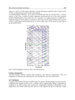
7.15.2 Breaking of a dam
This example is an attempt to model the breaking of a dam or more generally a flow
with large free surface motion by the ALE formulations described in the previous sections.
This problem, which has an approximate solution for an inviscid fluid flowing over a
perfect frictionless bed, presents a formidable challenge when this solution is applied to
mine tailings embankments. A detailed description of this problem can be found in Huerta
& Liu(1988).
The problem is solved without the restraints imposed by shallow water theory and
only the case of flow over a still fluid (FSF) is considered. Study on another case of flow
over a dry bed (FDB) can be found in the paper of Huerta & Liu(1988). The accuracy of
the ALE finite element approach is checked by solving the inviscid case, which has an
analytical solution in shallow water theory; then, other viscous cases are studied and

discussed.
Figure 7.8 shows a schematic representation of the flow over a still fluid The
dimensionless problem is defined by employing the following characteristic dimensions:
the length scale is the height of the dam, H, over the surface of the downstream still fluid;
the characteristic velocity, gH ,is chosen to scale velocities; and
ρgH
is the pressure
scale. The characteristic time is arbitrarily taken as the length scale over the velocity scale,
i.e. H / g . Consequently, if the fluid is Newtonian, the only dimensionless parameter
associated with the field equations is the Reynolds number, R
e
= H gH / ν
, where
ν
is
the kinematics viscosity. A complete parametric analysis may be found in Huerta (1987).
Since the problem is studied in its dimensionless form, H is always set equal to one.
Along the upstream and downstream boundaries a frictionless condition is
assumed, whereas on the bed perfect sliding is only imposed in the inviscid case (for
viscous flows the velocities are set equal to zero). In the horizontal direction 41 elements
of unit length are usually employed, while in the vertical direction one, three, five, or seven
layers are taken. depending on the particular case (see Figure 7.9). For the inviscid
analysis,
∆H = H =1
, as in Lohner et al (1984). In this problem both the Lagrange-Euler
matrix method and the mixed formulation are equivalent because an Eulerian description is
taken in the horizontal direction; in the vertical direction a Lagrangian description is used
along the free surface while an Eulerian description is employed everywhere else.
Figure 7.10 compares the shallow water solution with the numerical results
obtained by the one and three layers of elements meshes. Notice how the full integration of

the Navier-Stokes equations smoothes the surface wave and slows down the initial motion
of the flooding wave (recall that the Saint Venant equations predict a constant wave celerity,
gH , from t = 0). No important differences exists between the two discretizations (i.e.
one or three elements in depth); both present a smooth downstream surface and a clearly
separate peak at the tip of the wave. It is believed that this peak is produced in large part by
the sudden change in the vertical component of the particle velocity between still conditions
and the arrival of the wave, instead of numerical oscillations only. Figure 7.11 shows the
W.K.Liu, Chapter 7 67
difference between a Galerkin formulation of the rezoning equation, where numerical node
to node oscillations are clear, and a Petrov-Galerkin integration of the free surface equation
(i.e. the previous 4lx3 element solution). The temporal criterion (Hughes and Tezduyar,
1984) is selected for the perturbation of the weighting functions, and, as expected (Hughes
and Tezduyar, 1984; Hughes and Mallet, 1986), better results are obtained if the Courant
number is equal to one. In the inviscid dam-break problem over a still fluid, the second-
order accurate Newmark scheme (Hughes and Liu, 1978) is used (i.e.
γ
= 0.5 and β =
0.25), while in all of the following cases numerical damping is necessary (i.e.
γ
> 0.5)
because of the small values of
∆H
; this numerical instability is discussed later
The computed free surfaces for different times and the previous Generalized
Newtonian fluids are shown in Figures 7.14 and 7.15. It is important to point out that the
results obtained with the Carreau-A model and n = 0.2 are very similar to those of the
Newtonian case with R
e
= 300
, whereas for the Bingham material with µ

p
= 1×10
2
P
a
• s
the free surface shapes resemble more closely those associated with R
e
= 3000; this is
expected because the range of shear rate for this problem is from 0 up to 20-30
s
−1
It
should also be noticed that both Bingham cases present larger oscillations at the free surface
and that even for the µ
p
= 1×10
3
P
a
• s
case the flooding wave moves faster than that for
the Carreau models. Two main reasons can explain such behavior; first, unless
uneconomical time-steps are chosen, oscillations appear in the areas where the fluid is at
rest because of the extremely high initial viscosity (1000 µ
p
); second, the larger shear
rates occur at the tip of the wave, and it is in this area that the viscosity suddenly drops at
least two orders of magnitude, creating numerical oscillations.
Exercise 7.1

Observe that if the Jacobian described in Eq. (7.4.3a) is:
J = det
∂x
∂X




=ε
ijk
∂x
i
∂X
1
∂x
j
∂X
2
∂x
k
∂X
3
(7.4.11a)
where ε
ijk
is the permutation symbol, then
˙
J
becomes:
˙

J =
∂(v
1
, x
2
,x
3
)
∂(X
1
, X
2
, X
3
)
+
∂(x
1
,v
2
, x
3
)
∂(X
1
, X
2
, X
3
)

+
∂(x
1
, x
2
,v
3
)
∂(X
1
, X
2
, X
3
)
(7.4.11b)
where
W.K.Liu, Chapter 7 68
∂(a,b,c)
∂( X
1
, X
2
, X
3
)
=
∂a
∂X
1

∂a
∂X
2
∂a
∂X
3
∂b
∂X
1
∂b
∂X
2
∂b
∂X
3
∂c
∂X
1
∂c
∂X
2
∂c
∂X
3
(7.4.11c)
for arbitrary scalars a, b, and c, and v
i
=
˙
x

i
.
Using the chain rule on
∂v
1
∂X
j
, show that:
∂(v
1
, v
2
,v
3
)
∂( X
1
, X
2
, X
3
)
=
m =1
3
∑
∂v
1
∂x
m

∂(x
m
, x
2
,v
3
)
∂( X
1
, X
2
, X
3
)
=
∂v
1
∂x
1
J
(7.4.12a)
Similarly, show that:
˙
J = J v
k,k
(7.4.12b)
Exercise 7.2 Updated ALE Conservation of Angular Momentum
The principle of conservation of angular momentum states that the time rate of change
of the angular momentum of a given mass with respect to a given point, say the origin of
the reference frame, is equal to the applied torque referred to the same point. That is:

D
Dt
Ω
∫
x × ρ(x,t)v(x,t)dΩ =
Ω
∫
x × b(x,t)dΩ +
Γ
∫
x × t(x,t)dΓ
(7.4.13a)
It should be noticed that the left hand side of Eq. (7.4.13a) is simply
˙
H
.
(2a) Show that:
˙
H =
Ω
0
∫
D
Dt
(x) × (ρv)JdΩ
0
+
Ω
0
∫

x ×
D
Dt
(ρ vJ)dΩ
0
(7.4.13b)
=
Ω
∫
x ×
D
Dt
(ρv) + (ρv)div(v)




dΩ
Hint, in deriving the above equation, the following pieces of information have been used of
(1) x
,t[X]
= v
; (2) v × (ρ v) = 0 and (3) Eq. (7.3.6b).
Now, show that substituting Eqs. (7.4.13b) into Eq. (7.4.13a) yields:
W.K.Liu, Chapter 7 69

Ω
∫
x ×
D

Dt
(ρ v) + (ρ v)div(v)




dΩ
(7.4.14)
=
Ω
∫
x × b(x,t)dΩ +
Γ
∫
x ×(n⋅ σ)dΓ
(2b) Show that by employing the divergence theorem and the momentum equations given
in Eq. (7.4.6), the component form of Eq. (7.4.14) is:
Ω
∫
ε
ijk
σ
jk
dΩ = 0
(7.4.15)
(2c) If the Cauchy stress tensor,
σ
, is smooth within
Ω
, then the conservation of angular

momentum leads to the symmetry condition of the Cauchy (true) stress via Eq. (7.4.15)
and is given as:
σ
ij
= σ
ji
(7.4.16)
Exercise 7.3 Updated ALE Conservation of Energy
Energy conservation is expressed as (see chapter 3):
D
Dt
Ω
∫
ρEdΩ =
Γ
∫
σ
ji
n
j
v
i
dΓ +
Ω
∫
ρb
i
v
i
dΩ −

Γ
∫
q
i
n
i
dΓ +
Ω
∫
ρsdΩ
(7.4.17)
where q
i
is the heat flux leaving the boundary ∂Ω
x
. Recall that E is the specific total
energy density and is related to the specific internal energy e, by:
E = e +
V
2
2
(7.4.18a)
where e = e(θ,ρ) with θ being the thermodynamic temperature and
ρs
is the specific heat
source, i.e. the heat source per unit spatial volume and V
2
= v
i
v

i
. The Fourier law of heat
conduction is:
q
i
= −k
ij
θ
, j
(7.4.18b)
(3a) Show that the energy equation is (hint, use integration by parts and the divergence
theorem):
(ρE)
,t[χ]
+ (ρEc
j
)
,j
+ ρE
ˆ
v
j, j
= (σ
ij
v
i
)
, j
+ b
j

v
j
+ (k
ij
θ
,j
)
,i
+ ρs (7.4.19a)
(3b) If there is sufficient smoothness, time differentiate Eq. (7.4.19a) via the chain rule
and make use of the continuity equation to show that Eq. (7.4.19a) reduces to:
W.K.Liu, Chapter 7 70
ρ E
,t[χ]
+ E
, j
c
j
{ }
= (σ
ij
v
i
)
,j
+ b
j
v
j
+ (k

ij
θ
, j
)
,i
+ρs
(7.4.19b)
or, in index free notation:
ρ E
,t[χ]
+ c⋅ grad E
{ }
= div(v⋅σ)+ v⋅b+ div(k⋅grad θ ) + ρs
(7.4.19c)
(3c) Show that the above equations can be specified in the Lagrangian description by
choosing:
χ = X;
ˆ
φ =φ; c= 0; J=det
∂x
∂X




(7.4.20a)
and they are given by:
ρE
,t[χ]
= (σ

ij
v
i
)
,j
+ b
j
v
j
+(k
ij
θ
, j
)
,i
+ρs (7.4.20b)
or, in index free notation:
ρE
,t[χ]
= div(v⋅σ) + v⋅b+ div(k⋅grad θ) + ρs (7.4.20c)
(3d) Similarly, show that the Eulerian energy equation is obtained by choosing:
χ = x;
ˆ
φ =1; c=v;
ˆ
v =0; J = det
∂x
∂X





=1 (7.4.21a)
and they are given by:
ρ E
,t[χ]
+ E
, j
v
j
{ }
= (σ
ij
v
i
)
,j
+ b
j
v
j
+ (k
ij
θ
, j
)
,i
+ ρs
(7.4.21b)
or

ρ E
,t[χ]
+ v⋅ grad E
{ }
= div(v⋅σ)+ v⋅b+ div(k ⋅grad θ) + ρs
(7.4.21c)
Exercise 7.4
Show Eqs (7.13.10a), (7.13.10c), and (7.13.10d).
Exercise 7.5 Galerkin Approximation
Show the following Galerkin approximation by substituting these approximation
functions, Eqs (7.13.12), into Eqs. (7.13.10).
Exercise 7.6 The Continuity Equation
(6a) Show that:
M
p
˙
P +L
p
(P)+G
T
v = f
extp
(7.13.15a)
W.K.Liu, Chapter 7 71
where
M
p
is the generalized mass matrices for pressure;
L
p

is the generalized convective
terms for pressure; G is the divergence operator matrix; f
extp
is the external load vector; P
and v are the vectors of unknown nodal values for pressure and velocity, respectively; and
˙
P
is the time derivative of the pressure.
(6b) Show that:
M
AB
P
=
Ω
e
∫
1
B
N
A
p
N
B
p
dΩ
(7.13.15b)
L
A
P
=

Ω
e
∫
1
B
N
A
p
c
k
∂p
∂x
k
dΩ
(7.13.15c)
G
AB
P
=
Ω
e
∫
N
A
p
∂N
B
∂x
m
dΩ

(7.13.15d)
Example 7.2 1D Advection-Diffusion Equation
2P
e
φ
,x
− φ
,xx
= 0
P
e
= 1.5
τ = 0.438
∆x = 1
Exercise 7.7 The Momentum Equation
(7a) Show that:
Ma +L(v)+K
µ
v −GP = f
extv
(7.13.16a)
where
M
is the generalized mass matrices for velocity;
L
is the generalized convective
terms for velocity; G is the divergence operator matrix; f
extv
is the external load vector
applied on the fluid; K

µ
is the fluid viscosity matrix; P and v are the vectors of unknown
nodal values for pressure and velocity, respectively; and
˙
P
and a are the time derivative of
the pressure, and the material velocity, holding the reference fixed.
(7b) Show that:
M
AB
=
Ω
e
∫
ρN
A
N
B
dΩ
(7.13.16b)
L
A
=
Ω
e
∫
ρN
A
c
m

∂v
i
∂x
m
dΩ
(7.13.16c)
W.K.Liu, Chapter 7 72
K
µ
=
Ω
e
∫
B
T
DB dΩ
(7.13.16d)
where

B = B
1
LB
a
LB
NEN
[ ]
(7.13.17a)
B
a
T

=
∂N
a
∂x
1
∂N
a
∂x
2
0 0 0
∂N
a
∂x
3
0
∂N
a
∂x
1
∂N
a
∂x
2
0
∂N
a
∂x
3
0
0 0 0

∂N
a
∂x
3
∂N
a
∂x
2
∂N
a
∂x
1














(7.13.17b)
D =
2µ 0 0 0 0 0
0 µ 0 0 0 0

0 0 2µ 0 0 0
0 0 0 2µ 0 0
0 0 0 0 µ 0
0 0 0 0 0 µ














(7.13.17c)
Exercise 7.8 The Mesh Updating Equation
(8a) Show that:
ˆ
M
ˆ
v +
ˆ
L (x) −
ˆ
M v = f
extx

(7.13.18a)
where
ˆ
M
is the generalized mass matrices for mesh velocity;
ˆ
L
is the generalized
convective terms for mesh velocity; f
extx
is the external load vector; and
ˆ
v
is the vectors of
unknown nodal values for mesh velocity.
(8b) Show that:
ˆ
M
AB
=
ˆ
Ω
e
∫
ρ
ˆ
N
A
ˆ
N

B
d
ˆ
Ω
(7.13.18b)
The convective term is defined as follows:
(i) Lagrangian-Eulerian Matrix Method:
Define:
ˆ
c
i
= (δ
ij
− α
ij
)v
j
(7.13.19a)
(8c) Show that the convective term is:
W.K.Liu, Chapter 7 73
ˆ
L
A
=
ˆ
Ω
e
∫
ˆ
N

A
ˆ
c
m
∂x
i
∂χ
m
d
ˆ
Ω
(7.13.19b)
Exercise 6
Replacing the test function δv
i
by δv
i
+ τρc
j
δv
i
δx
j
, show that the streamline-
upwind/Petrov-Galerkin formulation for the momentum equation is:
0 =
Ω
∫
δv
i

ρ
∂v
i
∂t
χ
dΩ +
Ω
∫
δv
i
ρc
j
∂v
i
∂x
j
dΩ−
Ω
∫
∂(δv
i
)
∂x
i
PdΩ−
Ω
x
∫
δv
i

ρg
i
dΩ
+
Ω
∫
µ
2
∂(δv
i
)
∂x
j
+
∂(δv
j
)
∂x
i






∂v
i
∂x
j
+

∂v
j
∂x
i






dΩ−
Γ
∫
δv
i
h
j
dΓ
⇐ Galerkin
+
e=1
NUMEL
∑
Ω
e
∫
τ ρc
j
δv
i

δx
j
ρ
∂v
i
∂t
χ
+ ρc
j
∂v
i
∂x
j
−
∂σ
ij
∂x
j
−ρg
i






dΩ ⇐ StreamlineUpwind
References:
Belytschko, T. and Liu, W.K. (1985), "Computer Methods for Transient Fluid-Structure
Analysis of Nuclear Reactors," Nuclear Safety, Volume 26, pp. 14-31.

Bird, R.B., Amstrong, R.C., and Hassager, 0. (1977), Dynamics of Polymeric Liquids,
Volume 1: Fluid Mechanics, John Wiley and Sons, 458 pages.
Huerta, A. (1987), Numerical Modeling of Slurry Mechanics Problems. Ph.D Dissertation
of Northwestern University.
Hughes, T.J.R., Liu, W.K., and Zimmerman, T.K. (1981), "LagrangianEulerian Finite
Element Formulation for Incompressible Viscous Flows”, Computer Methods in Applied
Mechanics and Engineering, Volume 29, pp. 329-349.
Hughes, T.J.R., and Mallet, M. (1986), "A New Finite Element Formulation for
Computational Fluid Dynamics: III. The Generalized Streamline Operator for
Multidimensional AdvectiveDiffusive Systems," Computer Methods in Applied
Mechanics and Engineering, Volume 58, pp. 305-328.
Hughes, T.J.R., and Tezduyar, T.E. (1984), "Finite Element Methods for First-Order
Hyperbolic Systems with Particular Emphasis on the Compressible Euler Equations”,
Computer Methods in Applied Mechanics and Engineering, Volume 45, pp. 217-284.
W.K.Liu, Chapter 7 74
Hutter, K., and Vulliet, L. (1985), 'Gravity-Driven Slow Creeping Flow of a
Thermoviscous Body at Elevated Temperatures," Journal of Thermal Stresses, Volume 8,
pp. 99-138.
Liu, W.K., and Chang, H. G. (1984), "Efficient Computational Procedures for Long-
Time Duration Fluid-Structure Interaction Problems," Journal of Pressure Vessel
Technology, Volume 106, pp. 317-322.
Liu, W.K., Lam, D., and Belytschko, T. (1984), "Finite Element Method for
Hydrodynamic Mass with Nonstationary Fluid," Computer Methods in Applied
Mechanics and Engineering, Volume 44, pp. 177-211.
Lohner, R., Morgan, K., and Zienkiewicz, O.C. (1984), "The Solution of Nonlinear
Hyperbolic Equations Systems by the Finite Element Method," International Journal for
Numerical Methods in Fluids, Volume 4, pp. 1043-1063.
Belytschko, T. and Kennedy, J.M.(1978), ‘Computer models for subassembly
simulation’, Nucl. Engrg. Design, 49, 17-38.
Liu, W.K. and Ma, D.C.(1982), ‘Computer implementation aspects for fluid-structure

interaction problems’, Comput. Methos. Appl. Mech. Engrg., 31, 129-148.
Brooks, A.N. and Hughes, T.J.R.(1982), ‘Streamline upwind/Petrov-Galerkin
formulations for convection dominated flows with particular emphasis on the
incompressible Navier-Stokes equations’, Comput. Meths. Appl. Mech. Engrg., 32, 199-
259.
Lohner, R., Morgan, K. and Zienkiewicz, O.C.(1984), ‘The solution of non-linear
hyperbolic equations systems by the finite element method’, Int. J. Numer. Meths. Fluids,
4, 1043-1063.
Liu, W.K.(1981) ‘Finite element procedures for fluid-structure interactions with
application to liquid storage tanks’, Nucl. Engrg. Design, 65, 221-238.
Liu, W.K. and Chang, H.(1985), ‘A method of computation for fluid structure
interactions’, Comput. & Structures, 20, 311-320.
Hughes, T.J.R., and Liu, W.K.(1978), ‘Implicit-explicit finite elements in transient
analysis’, J. Appl.Mech., 45, 371-378.
Liu, W.K., Belytschko, T. And Chang, H.(1986), ‘An arbitrary Lagrangian-Eulerian
finite element method for path-dependent materials’, Comput. Meths. Appl. Mech. Engrg.,
58, 227-246.
Liu, W.K., Ong, J.S., and Uras, R.A.(1985), ‘Finite element stabilization matricesa
unification approach’, Comput. Meths. Appl. Mech. Engrg., 53, 13-46.
Belytschko, T., Ong,S J, Liu, W.K., and Kennedy, J.M.(1984), ‘Hourglass control in
linear and nonlinear problems’, Comput. Meths. Appl. Mech. Engrg., 43, 251-276.
W.K.Liu, Chapter 7 75
Liu, W.K., Chang, H, Chen, J-S, and Belytschko, T.(1988), ‘Arbitrary Lagrangian-
Eulerian Petrov-Galerkin finite elements for nonlinear continua’, Comput. Meths. Appl.
Mech. Engrg., 68, 259-310.
Benson, D.J.,(1989), ‘An efficient, accurate simple ALE method for nonlinear finite
element programs’, Comput. Meths. Appl. Mech. Engrg, 72 205-350.
Huerta, A. & Casadei, F.(1994), “New ALE applications in non-linear fast-transient solid
dynamics”, Engineering Computations, 11, 317-345.
Huerta, A. & Liu, W.K. (1988), “Viscous flow with large free surface motion”, Computer

Methods in Applied Mechanis and Engineering, 69, 277-324.
W.K.Liu, Chapter 7 76
Backup of the previous version
In section 7.1, a brief introduction of the ALE is given. In section 7.2, the kinematics in
ALE formulation is described. In section 7.3, the Lagrangian versus referential updates is
given. In section 7.4, the updated ALE balance laws in referential description is described.
In section 7.5, the strong form of updated ALE conservation laws in referenctial
description is derived. In section 7.6, an example of dam-break is used to show the
application of updated ALE. In section 7.7, the updated ALE is applied to the path-
dependent materials extensively where the strong form, the weak form and the finite
element decretization are derived. In this section, emphasize is focused on the stress
update procedure. Formulations for regular Galerkin method, Streamline-upwind/Petrov-
Galerkin(SUPG) method and operator splitting method are derived respectively. All the
path-dependent state variables are updated with a similar procedure. In addition, the stress
update procedures in 1D case are specified with the elastic and elastic-plastic wave
propagation examples to demonstrate the effectiveness of the ALE method. In section 7.8,
the total ALE method, the counterpart of updated ALE method, is studied.
7.1 Introduction
The theory of continuum mechanics (Malvern [1969], Oden [1972]) serves to establish
an idealization and a mathematical formulation for the physical responses of a material
body which is subjected to a variety of external conditions such as thermal and mechanical
loads. Since a material body B defined as a continuum is a collection of material particles
p, the purpose of continuum mechanics is to provide governing equations which describe
the deformations and motions of a continuum in space and time under thermal and
mechanical disturbances.
The mathematical model is achieved by labelling the points in the material body B by
the real number planes
Ω
, where
Ω

is the region (or domain) of the Euclidean space.
Henceforth, the material body B is replaced by an idealized mathematical body, namely, the
region
Ω
. Instead of being interested in the atomistic view of the particles p, the
description of the behavior of the body B will only pertain to the regions of Euclidean
space .
Equations describing the behavior of a continuum can generally be divided into four
major categories: (1) kinematic, (2) kinetic (balance laws), (3) thermodynamic, and (4)
constitutive. Detailed treatments of these subjects can be found in many standard texts.
The two classical descriptions of motion, are the Lagrangian and Eulerian descriptions.
Neither is adequate for many engineering problems involving finite deformation especially
when using finite element methods. Typical examples of these are fluid-structure-solid
interaction problems, free-surface flow and moving boundary problems, metal forming
processes and penetration mechanics, among others.
Therefore, one of the important ingredients in the development of finite element
methods for nonlinear mechanics involves the choice of a suitable kinematic description for
each particular problem. In solid mechanics, the Lagrangian description is employed
extensively for finite deformation and finite rotation analyses. In this description, the
calculations follow the motion of the material and the finite element mesh coincides with the
W.K.Liu, Chapter 7 77
same set of material points throughout the computation. Consequently, there is no material
motion relative to the convected mesh. This method has its popularity because
(1) the governing equations are simple due to the absence of convective effects, and
(2) the material properties, boundary conditions, stress and strain states can be accurately
defined since the material points coincide with finite element mesh and quadrature points
throughout the deformation. However, when large distortions occur, there are
disadvantages such as:
(1) the meshes become entangled and the resulting shapes may yield negative volumes,
and

(2) the time step size is progressively reduced for explicit time-stepping calculations.
On the other hand, the Eulerian description is preferred when it is convenient to model
a fixed region in space for situations which may involve large flows, large distortions, and
mixing of materials. However, convective effects arise because of the relative motion
between the flow of material and the fixed mesh, and these introduce numerical difficulties.
Furthermore, the material interfaces and boundaries may move through the mesh which
requires special attention.
In this chapter, a general theory of the Arbitrary Lagrangian-Eulerian (ALE)
description is derived. The theory can be used to develop an Eulerian description also. The
definitions of convective velocity and referential or mesh time derivatives are given. The
balance laws, such as conservation of mass, balances of linear and angular momentum and
conservation of energy are derived within the mixed Lagrangian-Eulerian concept. The
degenerations of the mixed description to the two classical descriptions, Lagrangian and
Eulerian, are emphasized. The formal statement of the initial/boundary-value problem for
the ALE description is also discussed.
7.2 Kinematics in ALE formulation
7.2.1 Mesh Displacement, Mesh Velocity and Mesh Acceleration
In order to complete the referential description, it is necessary to define the referential
motion; this motion is called the mesh motion in the finite element formulation.
The motion of the body B, which occupies a reference region
Ω
χ
, is given by
x
=
ˆ
φ (χ,t)= χ+
ˆ
u (χ,t) = φ(X,t)
(7.2.7)

This ALE referential(mesh) region Ω
χ
is specified throughout and its motion is defined by
the mapping function
ˆ
φ
such that the motion of χ ∈Ω
χ
at time t is denoted by χ ∈Ω
χ
and
ˆ
u (χ,t) is the mesh displacement in the finite element formulation. It is noted that even
thought in general the mesh function
ˆ
φ
is different from the material function
φ
, the two
motions are the same as given in Eq.(7.2.7). The corresponding velocity (mesh velocity)
and acceleration (mesh acceleration) are defined as :
ˆ
v =
∂x
∂t
[χ]
=x
,t[χ]
=
ˆ

u
,t[χ]
mesh velocity (7.2.8a)
W.K.Liu, Chapter 7 78
and
ˆ
a =
∂
ˆ
v
∂t
[χ]
=
ˆ
v
,t[χ]
mesh acceleration (7.2.8b)
The motion
ˆ
φ
is arbitrary and the usefulness of the referential descripation will depend on
how this motion is chosen.
Depending on the choice of
χ
, we can obtain the Lagranginan description by setting
χ = X
and
ˆ
φ = φ
, the Eulerian description by setting

χ = x
, and the ALE description by setting
ˆ
φ ≠ φ
. The general referential description is referred to as Arbitrary Lagrangian-Eulerian
(ALE) in the finite element formulation. In this description, the function
ˆ
φ
must be
specified such that the mapping between x and
χ
is one to one. With this assumption and
by the composition of the mapping (denoted by a circle), a third mapping is defined such
that

χ = ψ(X,t) =
ˆ
φ
−1
oφ(X,t)
(7.2.10)
Similarly, for this motion displacement, velocity and acceleration variables can be
defined.
However, this is not necessary. These displacement, velocity and acceleration
variables can instead be defined with the aid of the chain rule and the appropriate mappings.
The schematic set up of these descriptions in one-dimension is shown in Fig. 1, and a
summary of the three descriptions is given in Table 7.1.
Fig.7.2 is shown to compare the three descriptions further, where the 1D motion of the
material is specified as:
x

= (1− X
2
)t + X t
2
+ X
Fig 7.2 Comparsion of Lagranian, Eulerian, ALE description
References:
W.K.Liu, Chapter 7 79
Fried, I., and Johnson, A. R., [1988]. "A Note on Elastic Energy Density Function for
Largely Deformed Compressible Rubber Solids," Computer Methods in Applied
Mechanics and Engineering, 69, pp. 53-64.
Hughes, T. J. R., [1987]. The Finite Element Method, Linear Static and Dynamic Finite
Element Analysis, Prentice-Hall.
Malvern, L. E., [1969]. Introduction to the Mechanics of a Continuous Medium, Prentice-
Hall.
Noble, B., [1969]. Applied Linear Algebra, Prentice-Hall.
Oden, J. T., [1972]. Finite Elements of Nonlinear Continua, McGraw Hill.
REFERENCES
Belytschko, T., and Kennedy, J.M. (1978), "Computer Models for Subassembly
Simulation," Nuclear Engineering Design, Volume 49, pp. 17-38.
Belytschko, T., Kennedy, J.M., and Schoeberie, D.F. (1980), 'QuasiEulerian Finite
Element Formulation for Fluid Structure Interaction, 11 Journal of Pressure Vessel
Technology, American Society of Mechanical Engineers, Volume 102, pp. 62-69.
Belytschko, T. and Liu, W.K. (1985), "Computer Methods for Transient Fluid-Structure
Analysis of Nuclear Reactors," Nuclear Safety, Volume 26, pp. 14-31.
Bird, R.B., Amstrong, R.C., and Hassager, 0. (1977), Dynamics of Polymeric Liquids,
Volume 1: Fluid Mechanics, John Wiley and Sons, 458 pages.
Brugnot, G., and Pochet, R. (1981), "Numerical Simulation Study of Avalanches,"
Journal of Glaciology, Volume 27, Number 95, pp. 7788.
Brooks, A.N., and Hughes, T.J.R. (1982), "Streamline Upwind/PetrovGalerkin

Formulations for Convection Dominated Flows with Particular Emphasis on the
Incompressible Navier-Stokes Equations, " Computer Methods in Applied Mechanics and
Engineering-, Volume 32, pp. 199-259.
Carey, G.F., and Oden, J.T. (1986), Finite Elements: Fluid Mechanics, Volume VI of the
Texas Finite Element Series, Prentice Hall, 323 pages.
Chen, C., and Armbruster, J.T. (1980), "Dam-Break Wave Model: Formulation and
Verification," Journal of the Hydraulics Division,
American Society of Civil Engineers, Volume 106, Number HY5, pp.747-767.
Donea, J. (1983), "Arbitrary Lagrangian-Eulerian Finite Element Methods," Computational
Methods for Transient Analysis, Edited by T. Belytschko and T.J.R. Hughes, Elvesier
Science Publishers, pp. 473-516.
Donea, J. (1984), "A Taylor-Galerkin Method for Convective Transport Problems,"
International Journal for Numerical Methods in Engineering, Volume 20, pp. 101-119.
W.K.Liu, Chapter 7 80
Donea, J., Fasoli-Stella, P., and Giuliani, S. (1977), "Lagrangian and Eulerian Finite
Element Techniques for Transient Fluid Structure Interaction Problems," Transactions of
the 4th International Conference on Structural Mechanics in Reactor Technology, Paper
Bl/2.
Dressler, R.F. (1952), "Hydraulic Resistance Effect Upon the Dam-Break Functions,'
Journal of Research of the National Bureau of Standards, Volume 49, Number 3, pp. 217-
225.
Goring, D.G. (1978), Tsunamis-The Propagation of Long Waves onto a Shelf,
Dissertation submitted to the California Institute of Technology in partial fulfillment of the
requirements for the degree of Doctor of Philosophy, 337 pages.
Heinrich, J.C., Huyakorn, P.S., Zienkiewicz, O.C., and Mitchell, A.R. (1977), "An
Upwind Finite Element Scheme for Two-Dimensional Convective Transport,' International
Journal for Numerical Methods in Engineering, Volume 11, pp. 131-145.
Heinrich, J.C., and Zienkiewicz, O.C. (1979), "The Finite Element Method and
"Upwinding" Techniques in the Numerical Solution of Convection Dominated Flow
Problems,' in Finite Elements for-Convection Dominated Flow, Edited by T.H.R.

Hughes, American Society of Mechanical Engineers, Volume 34, pp. 105-136.
Hirt, C.W., Amsden, A.A., and Cook, J.L. (1974), " An Arbitrary Lagrangian Eulerian
Computing Method for All Flow Speeds,' Journal of Computational Physics, Volume 14,
pp. 227-253.
Huerta, A. (1987), Numerical Modeling of Slurry Mechanics Problems. Dissertation
submitted to Northwestern University in partial fulfillment of the requirements for the
degree of Doctor of Philosophy, 187 pages.
Huerta, A., and Liu, W.K. (1987), "Viscous Flow Structure Interaction," to appear in
Journal of Pressure Vessel Technology, American Society of Mechanical Engineers.
Hughes, T.J.R. (1978), 'A Simple Scheme for Developing Upwind Finite Elements,'
International Journal of Numerical Methods in Engineering, Volume 12, pp. 1359-1365.
Hughes, T.J.R., and Brooks, A.N. (1982), 'A Theoretical Framework for Petrov-
Galerkin Methods with Discontinuous Weighting Functions: Application to the Streamline-
Upwind Procedure," Finite Elements in Fluids, Edited by R.H. Gallagher et al, John Wiley
and Sons Ltd., Volume 4, pp. 47-65.
W.K.Liu, Chapter 7 81
Hughes, T.J.R., and Liu, W.K. (1978), 'Implicit-Explicit Finite Elements in Transient
Analysis' Journal of Applied Mechanics, Volume 45, pp. 371-378.
Hughes, T.J.R., Liu, W.K., and Zimmerman, T.K. (1981), "LagrangianEulerian Finite
Element Formulation for Incompressible Viscous Flows”, Computer Methods in Applied
Mechanics and Engineering, Volume 29, pp. 329-349.
Hughes, T.J.R., and Mallet, M. (1986), "A New Finite Element Formulation for
Computational Fluid Dynamics: III. The Generalized Streamline Operator for
Multidimensional AdvectiveDiffusive Systems," Computer Methods in Applied Mechanics
and Engineering” , Volume 58, pp. 305-328.
Hughes, T.J.R., and Tezduyar, T.E. (1984), "Finite Element Methods for First-Order
Hyperbolic Systems with Particular Emphasis on the Compressible Euler Equations”,
Computer Methods in Applied Mechanics and Engineering, Volume 45, pp. 217-284.
Hutter, K., and Vulliet, L. (1985), 'Gravity-Driven Slow Creeping Flow of a
Thermoviscous Body at Elevated Temperatures," Journal of Thermal Stresses, Volume 8,

pp. 99-138.
Jeyapalan, J.K. (1980), Analysis of Flow Failures of Mine Tailings Impoundements,
Dissertation submitted to the University of California, Berkeley, in partial fulfillment of the
requirements for the degree of Doctor of Philosophy, 298 pages.
Keentok, M., Milthorpe, J.F., and O'Donovan, E. (1985), "On the Shearing Zone Around
Rotating Vanes in Plastic Liquids: Theory and Experiment," Journal of Non-Newtonian
Fluid Mechanics, Volume 17, pp. 23-35.
Liu, W.K., Belytschko, T., and Chang, H. (1986), "An Arbitrary Lagrangian-Eulerian
Finite Element Method for Path Dependent Materials," Computer Methods in Applied
Mechanics and Engineering, Volume 58, pp. 227-246.
Liu, W.K., and Chang, H. G. (1984), "Efficient Computational Procedures for Long-
Time Duration Fluid-Structure Interaction Problems," Journal of Pressure Vessel
Technology, American Society of Mechanical Engineers, Volume 106, pp. 317-322.
Liu, W.K., and Chang, H. G. (1985), "A Method of Computation for Fluid Structure
Interaction," Journal of Computers and Structures”, Volume 20, Number 1-3, pp. 311-
320.
W.K.Liu, Chapter 7 82
Liu, W.K., Chang, H., and Belytschko, T. (1987), "Arbitrary Lagrangian-Eulerian
Petrov-Galerkin Finite Elements for Nonlinear Continua," to appear in Computer Methods
in Applied Mechanics and Engineering.
Liu, W.K., and Gvildys, J. (1986), 'Fluid Structure Interactions of Tanks with and
Eccentric Core Barrel," Computer Methods in-Applied Mechanics and Engineering,
Volume 58, pp. 51-57.
Liu, W.K., Lam, D., and Belytschko, T. (1984), "Finite Element Method for
Hydrodynamic Mass with Nonstationary Fluid," Computer Methods in Applied Mechanics
and Engineering, Volume 44, pp. 177-211.
Liu, W.K., and Ma, D. (1982), "Computer Implementation Aspects for Fluid Structure
Interaction Problems," Computer Methods in Applied Mechanics and Engineering, Volume
31, pp. 129-148.
Lohner, R., Morgan, K., and Zienkiewicz, O.C. (1984), "The Solution of Nonlinear

Hyperbolic Equations Systems by the Finite Element Method," International Journal for
Numerical Methods in Fluids, Volume 4, pp. 1043-1063.
Ma, D.C., Gvildys, J., Chang, Y.W. , and Liu, W.K. (1982), "Seismic Behavior of
Liquid-Filled Shells," Nuclear Engineering- and Design, Volume 72, pp. 437-455.
Malvern, L.E. (1965), Introduction to the Mechanics of a Continuous Medium. Prentice
Hall, Engelwood Cliffs, New Jersey.
Muto, K., Kasai, Y., Nakahara, M., and Ishida, Y. (1985), "Experimental Tests on
Sloshing Response of a Water Pool with Submerged Blocks," Proceedings of the 1985
Pressure Vessels and Piping Conference, Volume 98-7 (Fluid-Structure Dynamics), Edited
by S.J. Brown, American Society of Mechanical Engineers, pp. 209214.
Noh, W.F. (1964), "CEL: A Time-Dependent- Two-Space Dimensional Coupled
Eulerian-Lagrangian Code,' in Methods in Computational Physics, Volume 3, Edited by B.
Alder, S. Fernbach and M. Rotenberg, Academic Press, New York.
O'Donovan, E.J., and Tanner, R.I. (1984), "Numerical Study of the Bingham Squeeze
Film Problem,' Journal of Non-Newtonian FluidMechanics, Volume 15, pp. 75-83.
Ramaswamy, B., Kawahara, M., and Nakayama, T. (1986), "Lagrangian Finite Element
Method for the Analysis of Two-Dimensional Sloshing Problems," International Journal
for Numerical Methods in Fluids, Volume 6, pp. 659-670.
W.K.Liu, Chapter 7 83
Ritchmyer, R.D., and Morton, K.W. (1967), Difference Methods for 56 Initial-Value
Problems, Interscience, New York, 2nd edition.
Sakkas, J.G., and Strelkoff, T. (1976), 'Dimensionless Solution of Dam-Break Flood
Waves," Journal of the Hydraulics Division, American Society of Civil Engineers, Volume
102, Number HY2, pp. 171-184.
Strelkoff, T. (1969), "One Dimensional Equations for Open Channel Flow," Journal of the
Hydraulics Division, American Society of Civil Engineers, Volume 95, Number HY3, pp.
861-876.
Tangy, P., Fortin, M., and Choplin, L. (1984), 'Finite Element Simulation of Dip
Coating, II: Non-Newtonian Fluids," International Journal for Numerical Methods in
Fluids, Volume 4, pp. 459-475.

Whitham, G.B. (1955), "The Effects of Hydraulic Resistance in the DamBreak Problem,"
Proceeding-s of the Royal Society of London, Series A, Volume 227, pp. 399-407.
Zienkiewicz, O.C., and Bettess, P. (1978), "Fluid-Structure Dynamic Interaction and
Wave Forces. An Introduction to Numerical Treatment," International Journal of
Numerical Methods in Engineering, Volume 13, pp. 1-16.
1. Belytschko, T. and Kennedy, J.M., ‘Computer models for subassembly simulation’,
Nucl. Engrg. Design, 49 (1978), 17-38.
2. Liu, W.K. and Ma, D.C., ‘Computer implementation aspects for fluid-structure
interaction problems’, Comput. Methos. Appl. Mech. Engrg., 31(1982), 129-148.
3. Brooks, A.N. and Hughes, T.J.R., ‘Streamline upwind/Petrov-Galerkin formulations
for convection dominated flows with particular emphasis on the incompressible Navier-
Stokes equations’, Comput. Meths. Appl. Mech. Engrg., 32(1982), 199-259.
4. Lohner, R., Morgan, K. and Zienkiewicz, O.C., ‘The solution of non-linear
hyperbolic equations systems by the finite element method’, Int. J. Numer. Meths.
Fluids, 4(1984), 1043-1063.
5. Liu, W.K. ‘Finite element procedures for fluid-structure interactions with application to
liquid storage tanks’, Nucl. Engrg. Design, 65(1981), 221-238.
6. Liu, W.K. and Chang, H., ‘A method of computation for fluid structure interactions’,
Comput. & Structures, 20(1985), 311-320.
7. Hughes, T.J.R., and Liu, W.K., ‘Implicit-explicit finite elements in transient
analysis’, J. Appl.Mech., 45(1978), 371-378.
8. Liu, W.K., Belytschko, T. And Chang, H., ‘An arbitrary Lagrangian-Eulerian finite
element method for path-dependent materials’, Comput. Meths. Appl. Mech. Engrg.,
58(1986), 227-246.
9. Liu, W.K., Ong, J.S., and Uras, R.A., ‘Finite element stabilization matricesa
unification approach’, Comput. Meths. Appl. Mech. Engrg., 53(1985), 13-46.
10. Belytschko, T., Ong,S J, Liu, W.K., and Kennedy, J.M., ‘Hourglass control in
linear and nonlinear problems’, Comput. Meths. Appl. Mech. Engrg., 43(1984), 251-
276.
11. Liu, W.K., Chang, H, Chen, J-S, and Belytschko, T., ‘Arbitrary Lagrangian-

Eulerian Petrov-Galerkin finite elements for nonlinear continua’, Comput. Meths.
Appl. Mech. Engrg., 68(1988), 259-310.
W.K.Liu, Chapter 7 84
12. Benson, D.J., ‘An efficient, accurate simple ALE method for nonlinear finite element
programs’, Comput. Meths. Appl. Mech. Engrg, 72(1989), 205-350.
5
CHAPTER 8
ELEMENT TECHNOLOGY
by Ted Belytschko
Northwestern University
@ Copyright 1997
8.1 Introduction
Element technology is concerned with obtaining elements with better performance,
particularly for large-scale calculations and for incompressible materials. For large-scale
calculations, element technology has focused primarily on underintegration to achieve faster
elements. For three dimensions, cost reductions on the order of 8 have been achieved
through underintegration. However, underintegration requires the stabilization of the
element. Although stabilization has not been too popular in the academic literature, it is
ubiquitous in large scale calculations in industry. As shown in this chapter, it has a firm
theoretical basis and can be combined with multi-field weak forms to obtain elements which
are of high accuracy.
The second major thrust of element technology in continuum elements has been to
eliminate the difficulties associated with the treatment of incompressible materials. Low-
order elements, when applied to incompressible materials, tend to exhibit volumetric
locking. In volumetric locking, the displacements are underpredicted by large factors, 5 to
10 is not uncommon for otherwise reasonable meshes. Although incompressible materials
are quite rare in linear stress analysis, in the nonlinear regime many materials behave in a
nearly incompressible manner. For example, Mises elastic-plastic materials are
incompressible in their plastic behavior. Though the elastic behavior may be compressible,
the overall behavior is nearly incompressible, and an element that locks volumetrically will

not perform well for Mises elastic-plastic materials. Rubbers are also incompressible in
large deformations. To be applicable to a large class of nonlinear materials, an element
must be able to treat incompressible materials effectively. However, most elements have
shortcomings in their performance when applied to incompressible or nearly
incompressible materials. An understanding of these shortcomings are crucial in the
selection of elements for nonlinear analysis.
To eliminate volumetric locking, two classes of techniques have evolved:
1. multi-field elements in which the pressures or complete stress and strain fields
are also considered as dependent variables;
2. reduced integration procedures in which certain terms of the weak form for the
internal forces are underintegrated.
Multi-field elements are based on multi-field weak forms or variational principles; these are
also known as mixed variational principles. In multi-field elements, additional variables,
such as the stresses or strains, are considered as dependent, at least on the element level,
and interpolated independently of the displacements. This enables the strain or stress fields
to be designed so as to avoid volumetric locking. In many cases, the strain or stress fields
are also designed to achieve better accuracy for beam bending problems. These methods
cannot improve the performance of an element in general when there are no constraints
6
such as incompressibility. In fact, for a 4-node quadrilateral, only a 3 parameter family of
elements is convergent and the rate of convergence can never exceed that of the 4-node
quadrilateral. Thus the only goals that can be achieved by mixed elements is to avoid
locking and to improve behavior in a selected class of problems, such as beam bending.
The unfortunate byproduct of using multi-field variational principles is that in many
cases the resulting elements posses instabilities in the additonal fields. Thus most 4-node
quadrilaterals based on multi-field weak forms are subject to a pressure instability. This
requires another fix, so that the resulting element can be quite complex. The developemnt
of truly robust elements is not easy, particularly for low order elements. For this reason,
an understanding of element technology is useful to anyone engaged in finite element
analysis.

Elements developed by means of underintegration in its various forms are quite similar
from a fundamental and practical viewpoint to elements based on multi-field variational
principles, and the equivalence was proven by Malkus and Hughes() for certain classes of
elements. Therefore, while underintegration is more easily understood than multi-field
approaches, the methods suffer from the same shortcomings as multi-field elements:
pressure instabilities. Nevertheless, they provide a straightforward way to overcome
locking in certain classes of elements.
We will begin the chapter with an overview of element performance in Section 8.1.
This Section describes the characteristics of many of the most widely used elements for
continuum analysis. The description is limited to elements which are based on polynomials
of quadratic order or lower, since elements of higher order are seldom used in nonlinear
analysis at this time. This will set the stage for the material that follows. Many readers
may want to skip the remainder of the Chapter or only read selected parts based on what
they have learned from this Section.
Although the techniques introduced in this Chapter are primarily useful for controlling
volumetric locking for incompressible and nearly incompressible materials, they apply
more generally to what can collectively be called constrained media problems. Another
important class of such problems are structural problems, such as thin-walled shells and
beams. The same techniques described in this Chapter will be used in Chapter 9 to develop
beam and shell elements.
Section 8.3 describes the patch tests. These are important, useful tests for the
performance of an element. Patch tests can be used to examine whether an element is
convergent, whether it avoids locking and whether it is stable. Various forms of the patch
test are described which are applicable to both static programs and programs with explicit
time integration. They test both the underlying soundness of the approximations used in
the elements and the correctness of the implementation.
Section 8.4 describes some of the major multi-field weak forms and their application to
element development. Although the first major multi-field variational principle to be
discovered for elasticity was the Hellinger-Reissner variational principle, it is not
considered because it can not be readily used with strain-driven constitutive equations in

nonlinear analysis. Therefore, we will confine ourselves to various forms of the Hu-
Washizu principles and some simplifications that are useful in the design of new elements.
7
We will also describe some limitation principles and stability issues which pertain to mixed
elements.
To illustrate the application of element technology, we will focus on the 4-node
isoparametric quadrilateral element (QUAD4). This element is convergent for compressible
material without any modifications, so none of the techniques described in this Chapter are
needed if this element is to be used for compressible materials. On the other hand, for
incompressible or nearly incompressible materials, this element locks. We will illustrate
two classes of techniques to eliminate volumetric locking: reduced integration and multi-
field elements. We then show that reduced integration by one-point quadrature is rank
deficient, which leads to spurious singular modes. To stabilize these modes, we first
consider perturbation hourglass stabilization of Flanagan and Belytschko (1981). We then
derive mixed methods for stabilization of Belytschko and Bachrach (1986), and assumed
strain stabilization of Belytschko and Bindeman (1991). We show that assumed strain
stabilization can be used with multiple-point quadrature to obtain better results when the
material response is nonlinear without great increases in cost. The elements of Pian and
Sumihara() and Simo and Rifai() are also described and compared. Numerical results are
also presented to demonstrate the performance of various implementations of this element.
Finally, the extension of these results to the 8-node hexhedron is sketched.
8.2. Overview of Element Performance
In this Section, we will provide an overview of characteristics of various widely-used
elements with the aim of giving the reader a general idea of how these elements perform,
their advantages and their major difficulties. This will provide the reader with an
understanding of the consequences of the theoretical results and procedures which are
described later in this Chapter. We will concentrate on elements in two dimensions, since
the properties of these elements parallel those in three dimensions; the corresponding
elements in three dimension will be specified and briefly discussed. The overview is
limited to continuum elements; the properties of shell elements are described in Chapter 9.

In choosing elements, the ease of mesh generation for a particular element should be
borne in mind. Triangles and tetrahedral elements are very attractive because the most
powerful mesh generators today are only applicable to these elements. Mesh generators for
quadrilateral elements tend to be less robust and more time consuming. Therefore,
triangular and tetrahedral elements are preferable when all other performance characteristics
are the same for general purpose analysis.
The most frequently used low-order elements are the three-node triangle and the four-
node quadrilateral. The corresponding three dimensional elements are the 4-node
tetrahedron and the 8-node hexahedron. The detailed displacement and strain fields are
given later, but as is well-known to anyone familiar with linear finite element theory, the
displacement fields of the triangle and tetrahedron are linear and the strains are constant.
The displacement fields of the quadrilateral and hexahedron are bilinear and trilinear,
respectively. All of these elements can represent a linear displacement field and constant
strain field exactly. Consequently they satisfy the standard patch test, which is described in
Section 8.3. The satisfaction of the standard patch test insures that the elements converge
8
in linear analysis, and provide a good guarantee for convergent behavior in nonlinear
problems also, although there are no theoretical proofs of this statement.
We will first discuss the simplest elements, the three-node triangle in two dimensions,
the four-node tetrahedron in three dimensions. These are also known as simplex elements
because a simplex is a set of n+1 points in n dimensions. Neither simplex element
performs very well for incompressible materials. Constant-strain triangular and tetrahedral
elements are characterized by severe volumetric locking in two-dimensional plane strain
problems and in three dimensions. They also manifest stiff behavior in many other
cases, such as beam bending. For arbitrary arrangements of these elements, volumetric
locking is very pronounced for materials such as Mises plasticity. The proviso plane strain
is added here because volumetric locking will not occur in plane stress problems, for in
plane stress the thickness of the element can change to accommodate incompressible
materials. The consequences of volumetric locking are almost a complete lack of
convergence. In the presence of volumetric locking, displacements are underpredicted by

factors of 5 or more, so the results are completely worthless.
Volumetric locking does not preclude the use of simplex elements for incompressible
materials completely, for locking can be avoided by using special arrangements of the
elements. For example, the cross-diagonal arrangement of triangles shown in Fig.??
eliminates locking, Naagtegal et al. However, meshing in this arrangement is similar to
meshing quadrilaterals, so the benefits arising from triangular and tetrahedral meshing are
lost. In addition, this arrangement results in pressure oscillations, such as those described
subsequently for quadrilaterals.
When fully integrated, i.e. 2x2 Gauss quadrature for the quadrilateral, both the 4-node
quadrilateral and the hexahedron lock for incompressible materials. Volumetric locking can
be eliminated in these elements by using reduced integration, namely one-point quadrature,
or selective-reduced integration, which consists of one-point quadrature on the volumetric
terms and 2x2 quadrature on the deviatoric terms; this is described in detail later. The
resulting quadrilateral will then exhibit good convergence properties in the displacements.
However, the element still is plagued by one flaw: it exhibits pressure oscillations due to
the failure of the quadrilateral with modified quadrature to satisfy the BB-condition, which
is described later. As a consequence, the pressure field will often be oscillatory, with a
pattern of pressures as shown in fig, ??. This oscillatory pattern in the pressures is often
known as checkerboarding. Checkerboarding is sometimes harmless: for example, in
materials governed by the Mises law the response is independent of pressure, so pressure
oscillations are not very harmful, although they lead to errors in the elastic strains.
Checkerboarding can also be eliminated by filtering procedures. Nevertheless it is
undesirable, and a user of finite elements should at least be aware of its possibility with
these elements. Pressure oscillations also occur for the mixed elements based on multi-
field variational principles. In fact mixed elements are in many cases identical or very
similar in performance to selective reduced integration elements, since theoretically they are
in many cases equivalent, Malkus and Hughes(). Some stabilization procedures for BB
oscillations have been developed; they are described and discussed in Section ??.
In large scale computations, the fastest form of the quadrilateral and hexahedron is the
one-point quadrature element: it is often 3 to 4 times as fast as the selective-reduced

quadrature quadrilateral element. In three dimensions, the speedup is of the order of 6 to 8.
9
The one-point quadrature element also suffers from pressure oscillations, and in addition
possess instabilities in the displacement field. These instabilities are shown in Fig. ??, and
have various names: hourglassing, keystoning, kinematic modes, spurious zero energy
modes and chickenwiring are some of the appellations for these modes. The control of
these modes has been the topic of considerable research, and they can be controlled quite
effectively. In fact, the rate of convergence is not decreased by a consistent control of these
modes, so for many large scale calculations, one-point quadrature with hourglass control
are very effective. Hourglass control is described in Sections ???.
The next highest order elements are the 6-node triangle and the 8 and 9 node
quadrilaterals. The counterparts in three dimensions are the 10 node tetrahedron and the 20
and 27 node quadrilaterals. The 6-node triangle and 9-node quadrilateral have a complete
quadratic displacement field and complete linear strain field when the edges of the element
are straight. Ciarlet and Raviart() in a landmark paper proved that the convergence of these
elements is quadratic when the displacement of the midside nodes is small compared to the
length of the elements; whether the distortions introduced by a mesh in normal mesh
generation are small is often an open question. These elements satisfy the quadratic and
linear patch tests when the element sides are straight, but only the linear patch test when the
element sides are curved. In other words, these elements cannot reproduce a quadratic
displacement field exactly when the sides are not straight. Of course, curved sides are an
intrinsic advantage of finite elements, for they enable boundary conditions to be met for
higher order elements, but curved sides should only be used for exterior surfaces, since
their presence decreases the accuracy of the element. In nonlinear problems with large
deformations, the performance of these elements degrades when the midside nodes move
substantially; this had already been discussed in the one-dimensional context in Example
2.8.2. Element distortion is a pervasive difficulty in the use of higher order elements for
large-deformation analysis: the convergence rate of higher order elements degrades
significantly as they are distorted, and in addition solution procedures often fail when
distortion becomes excessive.

The 6-node triangle does not lock for incompressible materials, but it fails the BB
pressure stability test for incompressible materials. The 9-node quadrilateral when
developed appropriately by a mixed variational principle with a linear pressure field
satisfies the pressure stability test and does not lock. It is the only element we have
discussed so far which has flawless behavior for incompressible materials.
In summary, element technology deals with two major quirks:
1. volumetric locking, which prevents convergence for incompressible and nearly
incompressible materials;
2. pressure oscillations which result from the failure to meet the BB condition.
For low-order elements, the presence of one of these flaws is nearly unavoidable. The
quadrilateral with reduced integration and a pressure stabilization or pressure filter appears
to be the best of the low-order elements. When speed of computation is a consideration, a
stabilized quadrilateral with one-point quadrature appears to be optimal. Only the 9-node
quadrilateral and 27-node hexahedral are flawless elements for imcompressible materials,
and the fact that no flaws have been discovered so far does not preclude that none will ever
be discovered. Almost all of these difficulties are driven by incompressibility, and persist
10
for near-incompressiblity. When the material is compressible, or when considering two
dimensional plane stress, standard element procedure can be used.
Error Norms. In order to compare these elements further, it is worthwhile to study a
convergence theorem which has been proven for linear problems. Although this theorem
has not been proven for the nonlinear regime, it provides insight into element accuracy.
For the purpose of studying this convergence theorem, we will first define some norms
frequently used in error analysis of finite elements. These will also be used to evaluate
some of the element technology developed later in this Chapter.
Errors in finite element analysis are measured by norms. A norm in functional
analysis is just a way of measuring the distance between two functions. A norm of the
difference between a finite element solution and the exact solution to a problem is a measure
of the error in the solution. The most common norms for the evaluating the error in a finite
element solution are the L

2
norm and the error in energy. The L
2
norm of a vector function
f
i
x
( )
is defined by
f
i
x
( )
0
= f
i
x
( )
f
i
x
( )
dΩ
Ω
∫









1
2
(8.2.1)
where the subscript nought on the symbol for the norm designates the L
2
norm. It can be
seen that the L
2
norm is always positive, and measures an average or mean value of the
function. To use the L
2
norm for a measure of error for a finite element solution, we
denote the finite element solution for the displacement by u
h
x
( )
and the exact solution by
u x
( )
. The error in the finite element solution at any point can then be expressed by the
vector e x
( )
= u
h
x
( )
− u x

( )
. Since we seek a single number for the error, we will use the
magnitude of the vector e x
( )
. which is e x
( )
⋅ e x
( )
. Thus we can define the error in the
displacements by the L
2
norm as
e x
( )
0
= e x
( )
⋅ e x
( )
dΩ
Ω
∫









1
2
or u − u
h
0
= u − u
h
( )
⋅ u − u
h
( )
dΩ
Ω
∫








1
2
(8.2.2)
This error norm measures the average error in the displacements over the domain of the
problem. There are many other error norms. We have chosen to use this one because the
most powerful and most well known results are expressed in terms of this norm.
Furthermore, it gives a measure of error which is useful for engineering purposes.
The second norm we will consider are the norms in Hilbert space. The H

1
norm of a
vector function is defined by