Nonlinear Finite Elements for Continua and Structures Part 17 ppsx
Bạn đang xem bản rút gọn của tài liệu. Xem và tải ngay bản đầy đủ của tài liệu tại đây (70.29 KB, 27 trang )
T. Belytschko, Contact-Impact, December 16, 1998
37
ˆ
f
Iα
res
= 0 or M
IJ
ˆ
˙
v
Jα
=
ˆ
f
Iα
ext
−
ˆ
f
Iα
int
for I ∈Γ
c
(X.5.15)
The equation for the normal component at the contact interface nodes involves the first
and third terms of the first sum in (13) and gives
f
In
res
+
ˆ
G
IJ
T
λ
J
= 0 or M
IJ
˙
v
Jn
+ f
In
ext
− f
In
int
+
ˆ
G
IJ
T
λ
J
= 0 forI ∈Γ
c
(X.5.16)
To extract the equations associated with the Lagrange multipliers, we note that
the variations of the nodal Lagrange multipliers must be negative. Therefore the
inequality (5) implies
ˆ
G
IJ
v
Jn
≤ 0
(X.5.17)
In addition, we have from Eq. (4.6) the requirement that the test function for the Lagrange
multiplier field must be positive
λ( ζ,t) ≥ 0
(X.5.18)
The above inequality is difficult to enforce. For elements with piecewise linear
displacements along the edges, this condition is often enforced only at the nodes by
λ
I
≥ 0
. This simplification is only appropriate with piecewise linear approximations
since the local minima of the Lagrange multipliers then occur at the nodes.
The above equations, in conjunction with the strain-displacement equations and
the constitutive equation, comprise the complete system of equations for the semidiscrete
model. The semidiscrete equations consist of the equations of motion and the contact
interface conditions. The equations of motion for nodes not on the contact interface are
unchanged from the unconstrained case. On the contact interface, additional forces
ˆ
G
IJ
λ
J
which represent the normal contact tractions appear. In addition, the
impenetrability constraint in weak form (17) must be imposed. Like the equations
without contact, the semidiscrete equations are ordinary differential equations, but the
variables are subject to algebraic inequality constraints on the velocities and the Lagrange
multipliers. These inequality constraints substantially complicate the time integration,
since the smoothness which is implicitly assumed by most time integration procedures is
lost.
For purposes of implementation, it is convenient to write the above equations in
matrix form in global components. Let the interpenetration rate be defined in terms of the
nodal velocities by
γ =Φ
Ii
( X)v
Ii
( t)
(X.5.19)
where
Φ
Ii
( X) =
N
I
n
i
A
if IonA
N
I
n
i
B
if IonB
(X.5.20)
The contact weak term is then given by
10-37
T. Belytschko, Contact-Impact, December 16, 1998
38
δG
L
= δ( λ
I
Γ
c
∫
Λ
I
Φ
Jj
v
Jj
) dΓ = λ
T
Gv
(X.5.21a)
where
G
JjI
= Λ
I
Φ
Jj
dΓ
Γ
c
∫
G = Λ
Τ
ΦdΓ
Γ
c
∫
(X.5.21b)
The equations of motion can be written in matrix form by combining this form
with matrix forms of the internal, external and inertial power, which gives
δv
T
f
int
− f
ext
+ M
˙ ˙
d
( )
+δ v
T
G
T
λ
( )
= 0 ∀δv ∈U
h
∀δλ ∈J
h−
(X.5.22)
We will skip the steps represented by Eqs. (7-17) and invoke the arbitrariness of
δv
and
δλ
. The matrix forms of the equations of motion and the interpenetration condition are
M
˙ ˙
d + f
int
− f
ext
+ G
T
λ = 0
(X.5.23a)
Gv ≤ 0
(X.5.23b)
The construction of the interpolation, and hence the nodal arrangement, for the
Lagrange multipliers poses some difficulties. In general, the nodes of the two contacting
bodies are not coincident, as shown in Fig. 5.1. Therefore it is necessary to develop a
scheme to deal with noncontiguous nodes. One possibility is indicated in Fig. 5.1, where
the nodes for the Lagrange multiplier field are chosen to be the nodes of the master body
which are in contact. This is a simple
10-38
T. Belytschko, Contact-Impact, December 16, 1998
39
Ω
B
Ω
A
Ω
B
Ω
A
λ
λ
Figure. X.5.1. Nodal arrangements for two contacting bodies with noncontiguous nodes
showing (a) a Lagrange multiplier mesh based on the master body and (b) an independent
Lagrange multiplier mesh.
scheme, but when the nodes of body B are much more finely spaced a coarse nodal
structure for the Lagrange multipliers will lead to interpenetration. An alternative is to
place Lagrange multiplier nodes wherever a node appears in either body A or B, as shown
in Fig. 5.1b. The disadvantage of that scheme is that when nodes of A and B are closely
spaced, the Lagrange multiplier element is then very small. This can lead to ill-
conditioning of the equations.
X.5.3. Assembly of Interface Matrix. The G matrix can be assembled from
“element” matrices like any other global finite element matrix. To illustrate the
assembly procedure, let the nodal velocities and Lagrange multipliers of element e be
expressed in terms of the global matrices by
v
e
= L
e
v λ
e
= L
e
λ
λ
(X.5.24a)
with identical relations for the test functions
δv
e
= L
e
v δλ
e
= L
e
λ
δλ
Substituting into (18) gives
10-39
T. Belytschko, Contact-Impact, December 16, 1998
40
λ
T
Gv = λγdΓ
Γ
c
∫
= λγdΓ
Γ
e
c
∫
=
e
∑
λ
T
L
e
λ
( )
T
Φ
T
Λ
Γ
e
c
∫
dΓL
e
v
Since (18) must hold for arbitrary
˙
d
and
λ
it can be seen by comparing the first and last
term of the above that
G = L
e
λ
( )
T
G
e
L
e
,
e
∑
G
e
=
Γ
e
c
∫
Λ
T
φdΓ
(X.5.25)
Thus the assembly of G from G
e
is identical to assembly of global matrices such as the
stiffness matrix.
X.5.4. Lagrange Multipliers for Small-Displacement Elastostatics. We
will call the analysis of small-displacement problems with linear, elastic materials small-
displacement elastostatics. We have used the nomenclature of small-displacement,
elastostatics rather than linear elasticity because these problems are not linear due to the
inequality constraint on the displacements which arises from the contact condition. For
small-displacement elastostatics, the governing relations for the impenetrability constraint
can be obtained from the preceding by replacing the velocities by the displacements.
Thus Eq. (2.7) and (19) are replaced by
g
N
= u
A
− u
B
( )
⋅n
A
≤ 0 onΓ
c
g
N
=Φd
(X.5.26)
The discretization procedure is then identical to the above except for substituting
velocities by displacements and omitting the inertia, giving
δd
T
f
int
− f
ext
( )
+ δ d
T
Gλ
( )
= 0 ∀δd ∈U ∀δλ ∈J
−
(X.5.27)
Since the internal nodal forces are not effected by contact, for the small displacement
elastostatic problem they can be expressed in terms of the stiffness matrix by
f
int
= Kd
(X.5.26a)
Taking the variation of the second term and using the arbitrariness of
δd
and the
arbitrary but negative character of
δλ
gives
K G
T
G 0
d
λ
=
≤
f
ext
0
(X.5.27)
This is the standard form for Lagrange multiplier problems except that an equality has
been replaced by an inequality in the second matrix equation.
If we recall other Lagrange multiplier problems, two properties of this system
come to mind:
1. the system of linear algebraic equations is no longer positive definite;
10-40
T. Belytschko, Contact-Impact, December 16, 1998
41
2. the equations as given above are not banded and it is difficult to find an
arrangement of unknowns so that they are banded;
3. the number of unknowns is increased as compared to the system
without the contact constraints.
In addition, for the contact problem, the solution of the equations is complicated
by the presence of the inequalities. These are very difficult to deal with and often the
small-displacement, elastostatic problem is posed as a quadratic programming problem,
see Section ?. These difficulties also arise in the nonlinear implicit solution of contact
problems.
A major disadvantage of the Lagrange multiplier method is the need to set up a
nodal and element topology for the Lagrange multipliers. As we have seen in the simple
two dimensional example, this can introduce complications even in two dimensions. In
three dimensions, this task is far more complicated. In penalty methods we see there is
no need to set up an additional mesh.
In comparison to the penalty method, the advantage of the Lagrange multiplier
method is that there are no user-set parameters and the contact constraint can be met
almost exactly when the nodes are contiguous. When the nodes are not contiguous,
impenetrability can be violated slightly, but not as much as in penalty methods.
However, for high velocity impact, Lagrange multipliers often result in very noisy
solutions. Therefore, Lagrange multiplier methods are most suited for static and low
velocity problems.
X.5.5. Penalty Method for Nonlinear Frictionless Contact. The nonlinear
discretization is developed only for the second form of the penalty method, (X.4.47). In
the penalty method only the velocity field needs to be approximated. Again, the velocity
field is
C
0
within each body, but no stipulation of continuity between bodies need be
made. Continuity between bodies on the contact interface is enforced by the penalty
method. We only develop the weak penalty term
δ G
p
= δγp( g,γ) dΓ
Γ
c
∫
(X.5.28)
since the other weak terms are unchanged from the unconstrained problem. Substituting
δ G
P
= δv
T
φ
T
pdΓ
Γ
c
∫
≡δv
T
f
c
(X.5.29)
where φthe second equality defines
f
c
by
f
c
= φ
T
pdΓ
Γ
c
∫
(X.5.30)
Note the similarity of this formula to that for the internal forces; they express the same
thing, the relation between discrete forces and continuous tractions. Using (29) and (6) in
the weak form (4.28) with (4.39) the above definition of
f
c
gives
10-41
T. Belytschko, Contact-Impact, December 16, 1998
42
δ P = δv
T
f
res
+δv
T
f
c
(X.5.31)
So using the arbitrariness of
δv
and (5.6) gives
f
int
− f
ext
+ Ma +f
c
= 0
(X.5.32)
Thus in the penalty method the number of equations is unchanged from the unconstrained
problem. The inequalities (B1.3) do not appear explicitly among the discrete equations
but are enforced by appearance of the step function in the calculation of the contact
penalty forces by (30) and (4.38 ).
X.5.6. Penalty for Small-Displacement Elastostatics. For small-
displacement elastostatics, we replace velocities by displacements as previously.
Equation (4.43a) with
β
2
= 0
and (26b) give
p
= β
1
g
N
= β
1
φd
(X.5.33)
Substituting the above into (30) gives
f
c
= φ
T
p( g
N
)H (γ) dΓ
Γ
c
∫
= β
1
Γ
∫
φ
T
φH(γ) dΓd
or
f
c
= P
c
d, P
c
= β
1
Γ
∫
φ
T
φH( γ ) dΓ
(X.5.34)
Substituting (34) and (26a) into (32) after dropping the inertial term, gives,
( K+ P
c
) d = f
ext
(X.5.35)
This is a system of algebraic equations of the same order as the problem without contact
impact. The contact interface constraints appear strictly through the penalty forces P
c
d .
The algebraic equations are not linear because as can be seen from (34), the matrix P
c
involves the Heaviside step function of the gap, which depends on the displacements.
In contrast to the Lagrange multiplier methods it can be seen that:
1. the number of unknowns does not increase due to the enforcement of
the contact constraints.
2. the system equations remain positive definite since K is positive
definite and G is positive definite.
The disadvantage of the penalty approach is that the enforcement of the impenetrability
condition is only approximate and its effectiveness depends on the appropriateness of the
penalty parameters. If the penalty parameters is too small, excessive interpenetration
occurs causing errors in the solution. In impact problems, small penalty parameters
reduce the maximum computed stresses. We have seen some shenanigans in calculations
where analysts met stress criteria by reducing the penalty parameters. Picking the correct
10-42
T. Belytschko, Contact-Impact, December 16, 1998
43
penalty parameter is a challenging problem. Some guidelines are given in Section ?,
where we discuss implementation of various solution procedures with penalty methods.
X.5.7. Augmented Lagrangian. In the augmented Lagrangian method, the weak
contact term is
δ G
AL
= δ( λγ +
α
2
γ
2
) dΓ
Γ
c
∫
(X.5.36)
Using the approximation for the velocity
v(X,t)
and the Lagrange multiplier
λ( ξ, t)
gives
δ G
AL
= δ( λ
T
Λ
T
φv +
α
2
Γ
C
∫
v
T
φ
T
φv) dΓ
Taking the variations gives (X.5.37)
δ G
AL
= δλ
T
Gv+ δv
T
G
T
λ +δv
T
P
c
( α)v
(X.5.38)
where
P
c
( α)
is defined by (34). Writing out the weak form
δ P
AL
= δ P +δ G
AL
≥ 0
using Eqs. (36-38) then gives
f
int
− f
ext
+ Ma +G
T
λ +P
c
v = 0
(X.5.40a)
Gv ≤ 0
(X.5.40b)
Comparing Eqs. (40) with (23) and (35), we can see that the augmented
Lagrangian method gives contact forces which are a sum of those in the Lagrangian
method and the penalty method. The impenetrability constraint (40b), is the same as in
the Lagrange multiplier method.
For small-displacement elastostatics, we use the same procedure as before. We
change the dependent variables to displacements so we replace the nodal velocities by
nodal displacements, and using( ??) and (27a), the counterpart of Eqs. (39) and (40)
K +P
c
G
T
G O
d
λ
=
≤
f
ext
O
(X.5.41)
which further illustrates that the augmented Lagrangian method is a synthesis of penalty
and Lagrange multiplier methods , Eqs. (27) and (35).
X.5.8. Perturbed Lagrangian. The semidiscretization of the perturbed
Lagrangian formulation is obtained by using (4.45) with velocity and Lagrange multiplier
approximations are given by Eqs. (1) and (2), respectively. We won’t go through the
steps, since they are identical to the previous discretizations. The discrete equations are
f
int
− f
ext
+ Ma +G
T
λ = O
(X.5.42)
10-43
T. Belytschko, Contact-Impact, December 16, 1998
44
Gv− Hλ = O
(X.5.43)
Equation (42) corresponds to the momentum equation, Eq. (43) to the impenetrability
condition. The matrix
G
is defined by Eq. (21b) and
H =
1
β
Λ
T
Λ
Γ
c
∫
dΓ
(X.5.44)
The constraint equations (43) can be eliminated to yield a single system of equations.
Solving Eq.(43) for
λ
and substituting into (42) gives
f
int
− f
ext
+ Ma +G
T
H
−1
G = 0
(X.5.45)
The above is similar to the discrete penalty equation (35) with the penalty parameter β
appearing through H in (44). The last term in the above equations represents the contact
forces.
The semidiscrete equations for small-displacement elastostatics for the perturbed
Lagrangian methods are
K G
T
G −H
d
λ
=
f
ext
O
(X.5.46)
Comparing the above to the Lagrangian method, Eq. (27), we can see that it differs only
in the lower left submatrix, which is 0 in the Lagrangian method but consists of the
matrix H in the perturbed Lagrangian method.
10-44
T. Belytschko, Contact-Impact, December 16, 1998
45
BOX X.3 Semidiscrete Equations for Nonlinear Contact
f = f
ext
− f
int
Lagrange Multiplier
Ma −f + G
T
λ = 0, Gv≤ 0, λ( x) ≥ 0
Penalty
Ma −f + f
c
= 0, f
c
= Φ
T
p( g
N
)
Γ
c
∫
H ( g
N
)dΓ
Augmented Lagrangian
Ma −f + G
T
λ +P
c
v = 0, Gv ≤ 0
Perturbed Lagrangian
Ma −f + G
T
λ = 0, Gv− Hλ = 0
G = Λ
T
φ dΓ
Γ
c
∫
H = Λ
T
Λ dΓ P
c
=
Γ
c
∫
αφ
T
φ dΓ
Γ
c
∫
1
1 2
2
3
A
n
B
n
Ω
A
Ω
B
Figure X.5.1. One dimensional example of contact; example 1.
10-45
T. Belytschko, Contact-Impact, December 16, 1998
46
Example X.5.1. Finite Element Equations for One Dimensional
Contact-Impact. Consider the two rods shown in Fig. X.5.1. We consider a rod of
unit cross-sectional area. The contact interface consists of the nodes at the ends of the
rods, which are numbered 1 and 2. The unit normals, as shown in Fig. X.5.1, are
n
x
A
=1, n
x
B
=−1
. The contact interface in one-dimensional problems is rather odd since it
consists of a single point. The velocity fields in the two elements which border the
contact interface are given by
v( ξ,t) = N( ξ,t)
˙
d = ξ
A
, 1− ξ
B
, ξ
B
[ ]
˙
d
(X.5.47)
where the column matrix of nodal velocities is
˙
d
T
= v
1
v
2
v
3
[ ]
(X.5.48)
The G matrix is given by Eqs. (20) and (21); in a one-dimensional problem, the integral
is replaced by a single function value, with the function evaluated at the contact point:
G
T
= ξ
A
⋅n
A
, (1− ξ
B
)n
B
, ξ
B
[ ]
ξ
A
=1, ξ
B
=0
= ( 1)( +1), 1(−1), 0
[ ]
(X.5.49)
= 1, −1, 0
[ ]
The impenetrability condition in rate form, (23b), is given by
G
T
˙
d ≤ 0 or 1 −1 0
[ ]
˙
d = v
1
− v
2
≤ 0
(X.5.50)
The last equation can easily be obtained by inspection: when the two nodes are in contact,
the velocity of node 1 must be less or equal than the velocity of node 2 to preclude
overlap. If they are equal, they remain in contact, whereas when the inequality holds,
they release. These conditions are not sufficient to check for initial contact, which should
be checked in terms of the nodal displacements: x
1
− x
2
≥ 0
indicates contact has
occurred during the previous time step.
Since there is only one point of contact, only a single Lagrange multiplier appears
in the equations of motion. The equations of motion, Eqs. (BX.3.2) are then
M
11
M
12
M
13
M
21
M
22
M
23
M
31
M
32
M
33
˙ ˙
d
1
˙ ˙
d
2
˙ ˙
d
3
−
f
1
f
2
f
3
+
1
−1
0
λ
1
= 0
(X.5.51)
and
λ
1
≥ 0
(X.5.52)
10-46
T. Belytschko, Contact-Impact, December 16, 1998
47
The last terms in (51) are the nodal forces resulting from contact between nodes 1 and 2.
The forces on the nodes are equal and opposite and vanish when the Lagrange multiplier
vanishes. The equations of motion are identical to the equations for an unconstrained
finite element mesh except at the nodes which are in contact. The equations for a
diagonal mass matrix with unit area can be written as
M
1
a
1
− f
1
+λ
1
= 0
M
2
a
2
− f
2
−λ
1
= 0
(X.5.53)
M
3
a
3
− f
3
= 0
where
a
I
=
˙ ˙
d
I
.
The equations for small-displacement elastostatics, Eq. (27) can be written by
combining the G matrix, Eq. (49), with the assembled stiffness as in (27c) giving
k
1
0 0 1
0 k
2
−k
2
−1
0 −k
2
k
2
0
1 −1 0 0
d
1
d
2
d
3
λ
1
=
≥
f
1
f
2
f
3
0
ext
(X.5.54)
where k
I
is the stiffness of element I. The assembled stiffness matrix in the absence of
contact, i.e. the upper left hand 3x3 matrix, is singular, but with the addition of the
contact interface conditions, the complete 4x4 matrix becomes regular.
Penalty Method. To write the equation for the penalty method, we will use the
penalty law
p = βg = β( x
1
− x
2
) H(g) = β( X
1
− X
2
+ u
1
− u
2
) H( g)
. Then evaluating Eq.
(30) gives
f
c
= φ
T
p dΓ
Γ
c
∫
=
1
−1
0
βg (X.5.55)
The above integral consists of the integrand evaluated at the interface point since
Γ
c
is a
point. Equations (32) for a diagonal mass are then
M
1
a
1
− f
1
+βg = 0
M
2
a
2
− f
2
−βg = 0
(X.5.56)
M
3
a
3
− f
3
= 0
The equations are identical to that for the Lagrange multiplier method, (53) except that
the Lagrange multiplier is replaced by the penalty force.
10-47
T. Belytschko, Contact-Impact, December 16, 1998
48
To construct the small displacement, elastostatic equations for the penalty
method, we first evaluate P
c
by Eq. (34):
P
c
= β
1
φ
T
φH( g) dΓ
Γ
c
∫
=β
1
H ( γ)
+1
−1
0
+1 −1 0
[ ]
= β
1
H( g)
+1 −1 0
−1 +1 0
0 0 0
(X.5.57)
If we define
β = β
1
H ( g)
, and add P
c
to the linear stifness, then the resulting equations
are
k
1
+β −β
−β k
2
+β −k
2
−k
2
k
2
d
1
d
2
d
3
=
f
1
f
2
f
3
ext
(X.5.58)
It can be seen from the above equation that the penalty method simply adds a spring with
a spring constant
β
between nodes 1 and 2. The above equation is nonlinear since
β
is a
nonlinear function of g
= u
1
−u
2
.
10-48
T. Belytschko, Contact-Impact, December 16, 1998
49
y
x
1 2
3 4
l
Ω
A
Ω
B
n
A
n
B
Γ
C
Figure X.5.2
Example X2. Two Dimensional Example. Figure 2 shows two dimensional
bodies modeled by 4-node quadrilaterals which are in contact along a line parallel to the
x-axis. The approximations along the contact surface are written in terms of the element
coordinates of one of the master body A., which in this case is the identical to that of
body B. The velocity field along the contact interface is given by
v
x
( ξ ,t)
v
y
( ξ ,t)
=
N
1
0 N
2
0 N
3
0 N
4
0
0 N
1
0 N
2
0 N
3
0
N
4
v
(X.5.59)
where
v
T
= v
1x
v
1y
v
2 x
v
2y
v
3x
v
3y
v
4x
v
4 y
[ ]
T
(X.5.60)
10-49
T. Belytschko, Contact-Impact, December 16, 1998
50
N
1
= N
3
=1− ξ, N
2
= N
4
= ξ,ξ = x / l
(X.5.61)
The unit normals are given by n
A
= 0 −1
[ ]
T
,n
B
= 0 1
[ ]
T
so the Φ matrix is given by
Eq. (20):
Φ = N
1
n
1
A
N
1
n
2
A
N
2
n
1
A
N
2
n
2
A
N
3
n
1
B
N
3
n
2
B
N
4
n
1
B
N
4
n
2
B
[ ]
= −N
1
0 −N
2
0 N
3
0 N
4
0
[ ]
(X.5.62)
The Lagrange multiplier field is approximated by the same linear field (we will discuss
appropriate fields later)
λ( ξ ,t) =Λλ = N
1
N
2
[ ]
λ
1
λ
2
(X.5.63)
where the same shape functions as in (61) are used. The G matrix is given by
G = Λ
T
ΦdΓ =
l
6
0
−2 0 −1 0 2 0 1
0 −1 0 −2 0 1 0 2
Γ
c
∫
(X.5.64)
The terms of the rows resemble the terms of the consistent mass for a rod, and the
behavior for this Lagrange multiplier field is similar: a contact at node 1 results in forces
at node 2, and vice versa. Nodal forces due to contact are strictly in the y direction; all x-
components of forces from contact in this example will vanish since the odd rows of the
G matrix vanish. This is consistent with what is expected physically, since the contact
surface is along the x-direction and the contact interface is frictionless.
MISCELLANEOUS TOPICS
Regularization. The penalty approach may be thought of as a regularization of the
interface conditions; the exact solution of the impact of two rods leads to solutions
discontinuous in time, cf. Fig. . A regularization procedure in mathematics is a
procedure which by an artifact replaces a problem whose solutions are difficult to deal
with because of warts such as discontinuities or singularities by one with smoother, more
regular solutions. The classic example of regularization is von Neumann’s addition of
artificial viscosity to the Euler fluid equations to smooth shocks. Without this artificial
viscosity, solutions of the Euler equations in the vicinity of shocks by the central
difference method are so oscillatory that they look like lash. Von Neumann showed that
his regularization conserves momentum, so only part of the system is modified by
regularization.
The penalty method plays the same role as artificial viscosity in impact. With the
Lagrange multiplier method, the velocities are discontinuous in time at the point of
impact, and these discontinuities propagate through the body as waves and result in
considerable noise. The penalty regularization preserves momentum conservation, and
the other conservation equations are also observed exactly. It only relaxes one condition,
10-50
T. Belytschko, Contact-Impact, December 16, 1998
51
the impenetrability condition, by allowing some overlap of the two bodies. It is a small
price to pay for smoother solutions if the interpenetration is small.
The Curnier-Mroz plasticity models of friction can also be considered
regularization, in this case, of the discontinuous character of the friction laws. The
discontinuous nature of Coulomb friction can be gleamed from a simple illustration.
Consider an element on a rigid surface with interface tractions modeled by Coulomb
friction. A vertical force is applied to the top nodes, a horizontal force on the two left-
hand nodes as shown, and we neglect the deformability of the element. If the vertical
force is kept constant while the horizontal force has the time history shown, the velocity
will have the time history shown in Fig. Xd. The discontinuity in time arises because the
inequalities in the Coulomb friction law embody Heaviside step functions exactly as they
embodied in the interpenetration inequalities.
The Curnier-Mroz friction model eliminates the discontinuity as shown in Fig. X.
Regularization of Coulomb friction differs from regularization of interpenetration in that,
superficially at least, it smoothes the response by introducing additional mechanics to the
model, namely the asperities, whereas the relaxation of the interpenetrability condition
appears to be quite ad hoc and not motivated by physical arguments. In fact, one can also
attribute some interpenetration of the idealized bodies which comprise the models in
contact-impact problems to compression of asperities. Usually, however, the penalty
parameters are not chosen by such physical characteristics, but instead by the desirability
of eliminating frequencies above a certain threshold.
REFERENCES
T. Belytschko and M.O. Neal (1991), "Contact-Impact by the Pinball Algorithm with
Penalty and Lagrangian Methods," Int. J. for Numerical Methods in Engineering, 31.
547-572.
D.P. Bertsekas (1984), Constrained Optimization and Lagrange Multiplier Methods,
Academic Press, New York.
A. Curnier (1984), “A Theory of Friction,” Int. J. Solids and Structures, 20, 637-647.
Demkowicz and J. T. Oden (1981), On some existence and uniqueness results in contact
problems with nonlocal friction, Texas Institute of Computational Mechanics (TICOM)
Report 81-13, University of Texas at Austin.
N. Kikuchi and J.T. Oden, Contact Problems in Elasticity: A Study of Variational
Inequalities and Finite Element Methods, SIAM ????
R. Michalowski and Z. Mroz (1978), “Associated and non-associated sliding rules in
contact friction problems,” Archives of Mechanics, 30, 259-276.
P. Wriggers (1995), “Finite Element Algorithms for Contact Problems,” Archives of
Computational Methods in Engineering, 2,4, pp. 1-49.
10-51
T. Belytschko, Contact-Impact, December 16, 1998
52
P. Wriggers and C. Miehe (1994), “Contact Constraints within Coupled
Thermomechanical Analysis - a Finite Element Model,” Comp. Meth. in Appl. Mech.
and Eng., 113, 301-319.
10-52
T. Belytschko, Contact-Impact, December 16, 1998
53
ERRATA
1. p.38 should read
G
JjI
= Λ
I
Φ
Jj
dΓ
Γ
c
∫
G = Λ
Τ
ΦdΓ
Γ
c
∫
(X.5.21b)
2. in Box X.3 last equation should read
G = Λ
T
φ dΓ
Γ
c
∫
3. equation before (X.5.55) should read
p = βg = β( x
1
− x
2
) H(g) = β( X
1
− X
2
+ u
1
− u
2
) H( g)
X.6. EXPLICIT METHODS OF TIME INTEGRATION
In this Section we describe the procedures for treating contact impact with
explicit time integration. Explicit time integration is well suited to contact-impact
problems because the small time steps imposed by numerical stability can treat the
discontinuities in contact-impact. The large time steps made possible by unconditionally
stable implicit methods are not effective for discontinous response. Furthermore, contact-
impact also introduces discontinuities in the Jacobian, which impedes the convergence of
Newton methods.
Another advantage of explicit algorithms is that the bodies can first be integrated
completely independently, as if they were not in contact. This uncoupled solution
correctly indicates which parts of the body are in contact. The contact conditions are
imposed after the two bodies have been updated in an uncoupled manner; no iterations
are needed to establish the contact interface. An explicit algorithm with contact-impact is
almost identical to the algorithm described in Chapter X except that the bodies are
checked for interpenetration. In each time step, the displacements and velocities of those
nodes which have penetrated into another body are modified to reflect momentum
balance and impenetrability on the interface.
We will here describe several implementations of contact-impact algorithms in
explicit methods. Only the Lagrange multiplier and the penalty methods will be
considered. the issues to be discussed include: 1. the approximations for the Lagrange
multiplier fields; 2. structure of the algorithm; 3. effects of contact-impact methods on
numerical stability. We will also describe certain characteristics of explicit solutions
which arise from the physics and numerical characteristics of the contact-impact problem.
In order to illustrate the characteristics of contact-impact in a simple setting, we first
consider a one dimensional problem.
Example of Contact in One Dimension. The one-dimensional example is shown
in Fig. ??. We first consider the premise that uncoupled updates of bodies A and B
followed by modifications of the interpenetrating nodes for contact-impact lead to
consistent solutions. For the two points R and S, which correspond to nodes 1 and 2,
10-53
T. Belytschko, Contact-Impact, December 16, 1998
54
respectively, of bodies A and B, there are four possibilities during a contact-impact
problem
1. R and S are not in contact and do not contact during the time step;
2. R and S are not in contact but impact during the time step;
3. R and S are in contact and remain in contact;
4. R and S are in contact and separate during a time step, often known as release.
For case 3, the statement “remain in contact” does not imply that if two points must
remain contiguous, because relative tangential motion, or sliding, which separates
contiguous points is always possible. When two bodies remain in contact, they are
assumed not to separate.
All of these possibilities can be correctly accounted for by integrating the two
bodies independently as if they were not in contact and subsequently adjusting the
velocities and the displacements. The possibilities which need to be explained are cases
2, 3 and 4.
The governing equations for the nodes 1 and 2 have been given in Example Eq.
(53); although the problem shown in Fig. ?? is somewhat different, the equations for the
contact nodes are unchanged. We will show that when the velocities from the uncoupled
update predict initial or continuing contact, then the Lagrange multiplier
λ ≥ 0
. The
accelerations of nodes 1 and 2 when the two bodies are updated as uncoupled are
M
1
a
1
− f
1
= 0
, M
2
a
2
− f
2
= 0
where bars have been superposed on the accelerations to indicate that these are trial
accelerations computed with the uncoupled bodies, as can be seen from the absence of the
Lagrange multipliers. The central difference form of the update of Eqs. (53)
M
1
v
1
+
− M
1
v
1
−
−∆tf
1
+∆tλ =0
M
1
v
2
+
− M
1
v
2
−
−∆tf
2
−∆tλ =0
When the bodies contact during the time step, these equations must be solved with the
subsidiary condition v
1
+
= v
2
+
. Eliminating
λ
from the above equations by adding them
and using the equality v
1
+
= v
2
+
gives
v
1
+
= v
2
+
=
M
2
v
1
−
+ M
2
v
1
−
+∆t f
1
+ f
2
( )
M
1
+ M
2
where all unmarked variables are a time step n. By means of the above equations, the
updated velocities can be updated whenever impact occurs or the nodes were in contact in
the previous time step. The above equations can be recognized to be the well known
equations of conservation of mass for plastic impact of rigid bodies; more will be said on
this later.
10-54
T. Belytschko, Contact-Impact, December 16, 1998
55
We will now show that whenever the updated velocities of any nodes which
interpenetrate are computed by ( ), then the Lagrange multiplier will be positive, i.e. the
interface force will be compressive. In other words, if the two nodes are updated as if the
bodies were uncoupled and if the velocities are subsequently modified by (), then the
Lagrange multipliers will have the correct sign, This amounts to showing that
ifv
1
+
≥ v
2
+
, then
λ ≥ 0
.
Multiplying Eq top by M2 and Eq. bot by M1 and subtract bot form top; this gives
M
1
M
2
v
1
−
− v
2
−
( )
+∆t M
2
f
1
−M
1
f
2
( )
=λ∆t M
1
+M
2
( )
Substituting the expressions for f1 and f2 from () into the above and rearranging gives
∆t M
1
+ M
2
( )
M
1
M
2
λ = v
1
−
−v
2
−
( )
+∆t a
1
− a
2
( )
= v
1
+
−v
2
+
where the last equality is obtained by using the central difference formulas for the
uncoupled integration of the two bodies: v
I
+
= v
I
−
+∆ta
I
. The coefficient of
λ
is
positive, so the sign of the RHS gives the sign of
λ
. Thus Eq () has been demonstrated.
To examine this finding in more detail, we now consider the three of the cases
listed above (case 1 is trivial since it requires no modification of the nodal velocities since
there is no contact):
case 2 (not in contact /contacts during
∆t
): then
v
1
+
f v
2
+
and
λ ≥ 0
by Eq ()
case 3 (in contact/remains in contact): then
v
1
+
f v
2
+
and
λ ≥ 0
by Eq ()
case 4 (in contact/release during
∆t
): then
v
1
+
p v
2
+
and
λ p 0
by Eq ()
Thus the velocities obtained by uncoupled integration correctly predict the sign of the
Lagrange multiplier
λ
.
Two other interesting properties of explicit integration that can be learned from
this example are:
1. initial contact, i.e. impact cannot occur in the same time step as release;
2. energy is dissipated during impact;
The first statement rests on the fact that the Lagrange multiplier at time step n is
computed so that the velocities at time step n+1/2 match. Hence there is no mechanism
in an explicit method for forcing release during the time step in which impact occurs.
This property is consistent with the mechanics of wave propagation. In the mechanics of
impacting bodies, release is caused by rarefaction waves which are generated when the
compressive waves due to impact reflect from a free surface and reach the point of
contact. When the magnitude of these rarefaction is sufficient to cause tension across the
contact interface, release occurs. Therefore the minimum time required for release
10-55
T. Belytschko, Contact-Impact, December 16, 1998
56
subsequent to impact is two traversals of the distance to the nearest free surface. The
stable time step, you may recall, allows the any wave generated by impact to move at
most to the node nearest to the contact nodes. Therefore, in explicit time integration,
there is insufficient time in a stable time step for the waves to traverse twice the distance
to the nearest free surface.
The second statement can be explained by Eq. () which shows that the post-
impact velocities are obtained by the plastic impact conditions,for rigid bodies, which
always dissipate energy. The energy dissipated when two rods as shown in Fig.() are at
constant but equal velocities is given by
As can be seen from the above, the amount of dissipation decreases with the refinement
of the mesh. In the continuos impact problem, no energy is dissipated because the
condition of equal velocities after impact is limited to the impact surfaces. A surface is a
set of measure zero in three dimensions, so a change of energy over the surface has no
effect on the total energy. (For one-dimensional problems the impact surface is a point,
which is also a set of measure zero.) In a discrete model, the impacting nodes represent
the material layer of thickness h/2 adjacent to the contact surface. Therefore, the
dissipation in a discrete model is always finite. The correspondence between the
continuous model and the discrete model also substantiates the correctness of the plastic
impact condition. Since release cannot occur until the rarefaction waves reach the contact
interface, the velocities of the two contacting bodies must be equal until that time. Thus
it is inappropriate to use impact conditions other than perfectly plastic impact for discrete
models of continuous systems. It should be stressed that such arguments do not apply to
strictly multi-body models, where each node represents a body whose stiffness is not
modeled, or to structural models, where the thickness direction has no deformability. The
release and impact conditions are then more complex.
Penalty Method. The discrete equation at the impacting nodes for the two body problem
can be taken directly from those given in Eq. ():
M
1
a
1
− f
1
+ f
1
c
= 0
M
2
a
2
− f
2
− f
2
c
= 0
where the contact forces f
I
c
replace the Lagrange multiplier replace the Lagrange
multiplier in (). When the nodes are initially almost coincident, then X
1
= X
2
and the
interface normal traction can be written as
f
c
= p = β
1
g + β
1
g = β
1
( u
1
− u
2
) H(g) + β
2
( v
1
− v
2
) H(
˙
g )
The unitary condition is now approximately enforced by the step functions in the normal
contact force; it is violated since the normal traction is positive while the interpenetration
rate is positive, so its product no longer vanishes. The post-impact velocities are now
given by
10-56
T. Belytschko, Contact-Impact, December 16, 1998
57
The velocities of the two nodes are not equal since the penalty method only enforces the
impenetrability constraint approximately. As the penalty parameter is increased, the
condition of impenetrability is observed more closely. However, as indicated in the next
paragraph, in dynamics the penalty parameter cannot be made arbitrarily large.
The condition that release not occur in the same time step as impact, which has been
described to be a natural consequence of the physics of contact and numerical stability
conditions of explicit intergrators, is not automatically satisifed by the penalty method. If
the penalty force is very large, it is possible for the relative nodal velocity to reverse, so
that decreasing gap rate is is followed in the same time step by an increasing gap rate. In
view of the behavior of the continuous model described previously, which does not
permit release until rarefaction waves reflected from the free surfaces reach the contact
interface, this possibility in penalty methods does not appear physically correct. This
anomaly can be eliminated by placing an upper bound on the penalty force, so that the
impact is at most perfectly plastic. In other words, the penalty force should be bounded
so that the velocities at the end of the impact time step are given by (). This yields the
following upper bound on the contact force:
This bopund can be very useful since it provides a
In contrast to the Lagrange multiplier method, the penalty method usually
decreases the stable time step. An estimate of the stable time step can be made by using
the linear stiffness for the penalty method given in Eq. () in conjunction with the
eigenvalue element inequality. In using the element eigenvalue inequlitu, a group of
elements consisting of the penalty spring and the two surrounding elements should be
used, since the penalty element has no mass by itself and therefore has an infinite
frequency. This analysis shows that the stable time step for an interpenetration dependent
penalty is given by
whereα is given by
The decrease in the time step depends on the stiffness of the penalty spring. As the
interpenetration stifness b is increased, the stable time step decreases. As in the case of
the Lagrange multiplier method, this estimate of the stable time step is not a conservative
estimate, even though it is based on the element eigenvalue inequaality. The analysis
presumes linear behavior, whereas contact-impact is a very non-linear process.
EXPLICIT ALGORITHM
A flowchart for explicit time integration with contact-impact is shown in Box ??. As can
be seen from the flowchart, the contact impact conditions are enforced immediately after
the boundary conditions. Prior to the contact-impact step, all nodes in the model have
been updated as if they were not in contact, including the nodes which were in contact in
the previous time step. The nodes which are in contact are not treated differently in the
rest of the algorithm. Some difficulties may occur dus to making the contact-impact
10-57
T. Belytschko, Contact-Impact, December 16, 1998
58
modifications after the boundary condition enforcement. For example, for a pair of
contacting nodes on a plane of symmetry, it is possible for the contact-impact
modifications to result in violation of the condition that the velocities normal to the plane
of symmetry vanish. This can occur when the normal of the element adjacent to the plane
of symmetry does not lie in that plane. Therefore, boundary conditions sometimes have
to be imposed at contact nodes after the modifications.
The CONTACT module is limited to low-order elements in which the maximum
interpenetration always occurs of the nodes of the master or slave body. It is then only
necessary to check all nodes for interpenetration into elements of another body. The
second statement in the CONTACT nevertheless conceals many challenging tasks. In a
large model, on the order of 10
5
nodes may have to be checked against penetration into a
similar number of elements. Obviously a brute force approach to this task is not going to
work. Some of the strategies for dealing with this task are described in Section ?.
The
Box X.?
Flowchart for Explicit Integration with Contact-Impact
Main Program
1. initial conditions and setup:
t = 0, n = 0, setv
0
, σ
0
2. get nodal forces
f
t
= f
ext
− f
int
( )
t
3. velocity update: if
n f 0
,
v
∆t / 2
= v
0
+ M
−1
f
0
;
otherwise
v
t+∆t / 2
=v
t −∆t / 2
+ M
−1
f
t
4. displacement update:
d
t +∆t
=d
t
+ ∆tv
t+∆t/ 2
5. modify velocities and displacements for velocity boundary conditions
6. go to CONTACT
7. get
f
t+∆t
= f
ext
− f
int
( )
t+∆t
8. accelerations:
a
t
= M
−1
f
t
9. if
if t p END
, go to 3
CONTACT
1. find node-element pairs which are in contact;
2.
Lagrange multiplier method. The discrete equations for the system are obtained by
combining the semidiscrete equations with an explicit integration formula. For
simplicity, we consider here only the central difference method. Substituting an
expression for the accelerations at time step n, Eq.(), we obtain from () that
M v
n
+1 2
− v
n−12
( )
−f
n
+G
T
λ
n
=0
Referring to the flowchart in Box X, it can be seen that when the contact conditions are
enforced, the nodal forces at time step n are already known. However the Lagrange
10-58
T. Belytschko, Contact-Impact, December 16, 1998
59
multiplier are unknown. If we combine the above with the velocity constraint, Eq. () in
Box ?, we obtain
M ∆tG
T
G 0
v
n
+1 2
λ
n
=
≤
∆tf
n
+Mv
n−12
0
If a consistent mass matrix is used, solving for these variables appears to involve a
system of equations which is larger than the unconstrained system, since the Lagrange
multipliers have been added. In fact, for most systems, the size of the matrix can be
reduced substantially, since trial values of
v
n+12
are already known and only the
velocities of nodes on the contact interface are modified by contact .
In the above, everything on the right hand side is known at time step n when the
modifications for the contact are made. The unknowns are
λ
n
and
v
n+12
, although trial
values for the nodal velocities have already been obtained by the uncoupled update. The
solution for the Lagrange multipliers is obtained by first solving the top of the above
equation for
v
n+12
and then solving for
λ
n
, which gives
GM
−1
G
T
λ
n
≤ − M
−1
f
n
+
1
∆t
v
n+12
( )
≡rw
When the mass matrix is diagonal, the solution for the Lagrange multipliers can
be streamlined by taking advantage of the fact that the inverse of the mass matrix consists
of the reciprocals of the diagonal terms. To preserve the symmetric structure of the
equations we take the square root of the mass matrix and multiply G, and define the
resulting matrix as
G
:
G =M
−12
G G
ab
= M
ad
−12
G
db
Equations () can then be written as
G G
T
λ
n
=r
An interesting characteristic of these equations is that they are already in the form of a
triangulation. It is only necessary to eliminate all terms of the
G
matrix to obtain a
matrix from which the solution can easily be found. Moreover, the above equations
involve only the nodes on the contact interfaces. Thus the system of equations to be
solved is usually much smaller than the complete model. Nevertheless, for large-scale
explicit solutions, the burden of solving these equations is too great, so simplifications are
usually made to avoid solving these equations; these are discussed later.
Lagrange multiplier interpolation. In order to develop explicit forms of Eq.(), the
interpolation for the Lagrange multipliers must be defined. We have already mentioned
in Section X.5.2 that the construction of these interpolants can be complicated when the
nodes of the bodies are noncontiguous. As indicated there, two possibilities are: 1. the
master body mesh is chosen to be the l mesh; 2. construct a new mesh. Examples of the
G matrix for noncontiguous nodes have already been described in Example XX. We now
10-59
T. Belytschko, Contact-Impact, December 16, 1998
60
explore the consequences of various l approx imations and their effects on computational
efficency.
The implementation of implicit time integration and statics will be combined
because the procedure are almost identical. The reader is urged to consult Sections X,
where these topics are discussed for problems without contact. As in the aforementioned,
both classes of problems are treated by the Newton method.
In the Newton method, the solution to the discrete equations is found by using a
local linear model for the nonlinear equations. The linear model is based on a
linearization of the governing discrete equations. We will consider the Lagrange
multiplier methods and the penalty methods. In both cases, as before, we write the
nonlinear equations in the form
f (d,
˙
d ,λ) = 0
where
d,
˙
d , and λ
are, respectively, the nodal displacements, nodal velocities, and
discrete Lagrange multipliers at time
t +∆t
;
λ
appears only in the Lagrange multiplier
method. The internal force is only a function of d, i.e. the material is rate-independent.
The extension to rate dependent materials involves a combination of the techniques
described here and in Section X, but they obscure the effects of contact-impact, so are
omitted in this exposition.
In the Lagrange multiplier method the governing equations are
0 = f ( d,
˙
d ,λ,t) = M
˙ ˙
d (t) + f
int
( d) − f
ext
( d,t) −G( d) λ(t)
where the independent variables are indicated in the above. All of the above terms are
functions of time since d
= d t
. The development is restricted to rate-independent
materials, so the internal nodal forces are only functions of the nodal displacements, see
Section X.
We now expand the nodal forces by the chain rule, giving
10-60
T. Belytschko, Contact-Impact, December 16, 1998
61
n
A
A
n
B
A
X
e
^
e
X
B
^
V
B
V-
γ
T
γ
N
γ
Ω
Ω
A
B
Figure 4. Illustration of nomenclature in a two dimensional contact problem.
An interesting simplification of the above example is shown in Fig. . The
equations for this system can be obtained by just eliminating rows 1 and 3 and columns 1
and 3, giving
k
2
−1
−1 0
d
1
λ
1
=
f
1
0
The potential energy
Π( d, λ) =
1
2
k
2
d
2
− f
1
d
is plotted for f
1
=
in Fig. as a function of d
and
λ
; to obtain the plot, Eqs. ( ) have been solved.
10-61