Niche Modeling: Predictions From Statistical Distributions - Chapter 4 pptx
Bạn đang xem bản rút gọn của tài liệu. Xem và tải ngay bản đầy đủ của tài liệu tại đây (156.06 KB, 19 trang )
Chapter 4
Topology
The fo cus of topology here is the study of the subset structure of sets in the
mathematical spaces. Top ology can be used to describe and relate the different
spaces used in niche modeling. A top ology is a natural internal structure,
precisely defining the entire group of subsets produced by standard operations
of union and intersection. Of particular importance are those subsets, referred
to as open sets, where every element has a neighborhood also in the set. More
than one topology in X may be possible for a given set X.
Examples of subsets in niche modeling that could form topologies are the
geographic areas potentially occupied by a species, regions in environmental
space, groups of species, and so on.
Application of topological set theory helps to identify the basic assump-
tions underlying niche modeling, and the relationships and constraints be-
tween these assumptions. The chapter shows the standard definition of the
niche as environmental envelopes around all ecologically relevant variables is
equivalent to a box topology. A proof is offered that the Hutchinsonian en-
vironmental envelope definition of a niche when extended to large or infinite
dimensions of environmental variables loses desirable topological properties.
This argues for the necessity of careful selection of a small set of environmental
variables.
4.1 Formalism
The three main entities in niche modeling are:
S: the species,
N: the niche of environment variables, and
B: geographic space, where the environmental variables are defined.
.
45
© 2007 by Taylor and Francis Group, LLC
46 Niche Modeling
The relationships between these entities constitute whole fields of study in
themselves. Most applications of niche modeling fall into one of the categories
in Table 4.1.
TABLE 4.1: Links between geographic, environmental and species
spaces.
S N B
S interspecies relationships − −
N habitat suitability correlations −
B range predictions geographic information autocorrelation
Niche modeling operates on the collection of sets within these spaces. That
is, a set of individuals collectively termed a species, occupies a set of grid cells,
collectively termed its range, of similar environmental conditions, termed its
niche. Thus a niche model N is a triple:
N = (S, N, B)
The niche model is a general notion applicable to many phenomena. Here
are three examples:
• Biological species: e.g. the mountain lion Puma concolor, the environ-
ment variables might be temperature and rainfall, and space longitude
and latitude.
• Consumer products: e.g. a model of digital camera, say the Nikon
D50, environment variables for a D50 might be annual income and years
of photographic experience, and space the identities of individual con-
sumers.
• Economic event: e.g. a phenomenon such as median home price in-
creases greater than 20%, the variables relevant to home price increases
would be proximity to coast, family income, and the space of the metropoli-
tan areas.
A niche model can vary in dimension. Here are some examples of dimensions
of the geographic space B:
• zero dimensional such as a set, e.g. survey sites or individual people,
• one dimensional such as time, e.g. change in temperature or populations,
© 2007 by Taylor and Francis Group, LLC
Topology 47
• two dimensional such as a spatial area, e.g. range of a species,
• three dimensional such as change in range over time.
While examples of contemporary niche modeling can be seen in each of these
dimensions, many examples in this book are one dimensional, particularly
in describing the factors that introduce uncertainty into models, because a
simpler space is easier to visualize, analyze and comprehend. All results should
extend to studies in higher dimensions.
Dimensions of environmental space N, in Chapter 4, concern the implica-
tions of extending finite dimensional niche concepts into infinite dimensions.
Dimensions of species, one species for each dimension, relates to the field of
community ecology through inter-specific relationships.
Here we restrict examples to one species, and one S dimension.
4.2 Topology
There are a number of other ways to describe niche modeling. There are
a rich diversity of methods to predict species’ distribution and they could be
listed and described. Alternatively, biological relationships between species
and the environment could be emphasized, and approaches from population
dynamics used as a starting point. While useful, these are not the approaches
taken in this book, preferring to adhere to examination of fundamental prin-
ciples behind niche modeling.
Top ology is concerned with the study of qualitative prop erties of geometric
structures. One of the ways to address the question – What is niche modeling?
– is to study its topological properties.
4.3 Hutchinsonian niche
Historically, the quantitative basis of niche modeling lies in the Hutchinso-
nian definition of a niche [Hut58]. Here that set of environmental characteris-
tics where a species is capable of surviving was described as a ‘hypervolume’ of
an n-dimensional shape in n environmental variables. This is a generalization
of more easily visualizable lower dimensional volumes, i.e.:
© 2007 by Taylor and Francis Group, LLC
48 Niche Modeling
• one, an unbroken interval on the axis of an environmental variable, rep-
resenting the environmental limits of survival of the species,
• two, a rectangle,
• three, a box,
• n dimensions, hyp ervolumes.
This formulation of the niche has been very influential, in part because in
contrast to more informal definitions of the niche, it is easily operationalized
by simply defining the limits of observations of the species along the axes of
a chosen set of ecological factors.
4.3.1 Species space
Hutchinson denotes a species as S
1
so the set of species is therefore denoted
S. In its simplest form the values of the species S
1
are a two valued set,
presence or absence:
S
1
= {0, 1}
Alternatively the presence of a species could be defined by probability:
S
1
= {p|p ∈ [0, 1]}
4.3.2 Environmental space
Using the notation of Hutchinson the niche is defined by the limiting values
on independent environmental variables such as x
1
and x
2
. The notation used
for the limiting values are x
1
, x
1
and x
2
, x
2
for x
1
and x
2
respectively. The
area defined by these values corresponds to a possible environmental state
p ermitting the species to exist indefinitely.
Extending this definition into more dimensions, the fundamental niche of
sp ecies S
1
is described as the volume defined by the n variables x
1
, x
2
, , x
n
when n are all ecological factors relative to S
1
. This is called an n-dimensional
hypervolume N
1
.
© 2007 by Taylor and Francis Group, LLC
Topology 49
4.3.3 Topological generalizations
The notion Hutchinson had in mind is possibly the Cartesian product. If
sets in environmental variables x
i
are defined as sets of spaces X
i
, then N
1
is
a subset of the Cartesian product X of the set X
1
, , X
n
, denoted by
X = X
1
× × X
n
, or
X =
n
i=1
X
i
In a Cartesian product denoted by set X, a point in an environmental region
is an n-tuple denoted (x
1
, x
n
).
The environmental region related to a species S
1
is some subset of the entire
Cartesian space of variables X. The collection of sets has the form
i∈J
X
i
Setting a potentially infinite number i ∈ J to index the sets, rather than
a finite i equals 1 to n is a slight generalization. The construct captures the
idea that the space X
i
could consist of an infinite number of intervals. This
generalizes the n-dimensional hypervolume for a given species in S, so that
the space may encompass a finite or infinite number of variables.
Another generalization is to define each environmental variable x
i
as a topo-
logical space. A topological space T provides simple mathematical properties
on a collection of open subsets of the variable such that the empty set and
the whole set are in T, and the union and the intersection of all subsets are
in T. The set of open intervals:
(x
i
, x
i
) where x
i
, x
i
∈ R
is a topological space, called the standard topology on R.
Where each of the spaces in X
i
is a topology, this generates a topology
called a box topology, describing the box-like shape created by the intervals.
An element of the box topology is possibly what Hutchinson described as the
the n-dimensional hypervolume N
1
defining a niche.
4.3.4 Geographic space
There are differences between the environmental space N and the geograph-
ical space B. While the distribution of a species may be scattered over many
© 2007 by Taylor and Francis Group, LLC
50 Niche Modeling
discrete points in B, the shape of the distribution in N should be fairly com-
pact, representing the tendency of a species to be limited to a fairly small
environmental region. Perhaps the relevant concept from topology to de-
scribe this characteristic is connected. When the space N is connected, there
is an unbroken path between any two points. However, the same is not true
of the physical space B where populations could be isolated from each other.
4.3.5 Relationships
There is a particular type of relationship between N and B. Every species
with a non-empty range should produce a non-empty niche in the environmen-
tal variables. Moreover, a single point in the niche space N will have multiple
lo cations in the geographic space B, but not vice versa.
The relationship of niche to geography is a function. A function f is a rule
of assignment, a subset r of the Cartesian product of two sets B × N , such
that each element of B appears as the first coordinate of at most one ordered
pair in r. In other words, f is a function, or a mapping from B to N if every
p oint in B produces a unique point in N:
f : B −→ N
The inverse is not true, as a point in N can produce multiple points in B ,
those geographic points with the same niche, due to identical environmental
values.
One generalization used extensively in machine learning is to assume a set
of real-valued functions f
1
, , f
n
on B known as features such as the variable
itself, the square, the product of two features, thresholds and binary features
for categorical environmental variables [PAS06]. A binary feature takes a value
of 1 wherever the variable equals a specific categorical value, and 0 otherwise.
In another functional relationship g from N to S, each species occupies
multiple niche locations, but one niche lo cation has a distinct value for the
sp ecies space S, such as a probability.
g : N −→ S
Similarly, there is a functional relationship h from B to S where each species
may occupy multiple geographic points, but there is a unique value of a species
at each point.
h : B −→ S
© 2007 by Taylor and Francis Group, LLC
Topology 51
The natural mappings h from physical range B to the species S are referred
to as the observations. An alternative mapping, from B via the niche N to
S, is referred to as the prediction of the model. The similarity between these
mappings is the basis of assessments of accuracy.
g(f(B)) ∼ h(B).
4.4 Environmental envelope
We now consider how to operationalize these theoretical set definitions.
The approach of defining limits for each of the environmental variables
captures the sense of a niche as understood by ecologists: that the occurrence
of species should be limited by a range of environmental factors, and that
an envelope around those ranges would have predictive utility. This approach
was used in environmental envelopes, one of the first niche modeling tools first
used in an early study of the distribution of snakes in Australia by Henry Nix
[Nix86].
However, the approach has some practical problems.
4.4.1 Relevant variables
The Hutchinsonian definition suggests that the box continues in n-dimensions
until all ecological factors relevant to S
i
have been considered [Hut58].
There are a number of problems with this definition. One problem stems
from the vagueness of what is meant by an ecologically relevant factor. The
formalism provides no way to weight variables by importance, or exclude vari-
ables from the niche. Another problem is the number of potentially relevant
ecological factors is unlimited.
4.4.2 Tails of the distribution
The environmental envelope defines limits for the species largely by the
tails of the probability distribution. The tails of a probability distribution
usually have the smallest probabilities, the least numbers of samples, and
hence estimated with the least certainty. Hence a definition based on limits
© 2007 by Taylor and Francis Group, LLC
52 Niche Modeling
must be statistically uncertain, or at least less certain than a range that was
defined, say, via a type of confidence limits using mean values and variance.
Often to reduce the variability of the range limits the niche includes only
the 95% percentile of locations from B. Unfortunately this approach pro-
duces a progressive reduction in ecological area with each variable, leading
to underestimation of species’ potential ranges [BHP05]. Niche descriptions
such as based on Mahalanobis distances allow more flexible descriptions of the
distribution and have been shown to be more accurate [FK03].
4.4.3 Independence
The box-like shape only applies to independent variables, but species rarely
fit within a sharp box-like shape. Niche descriptions based on more flexible
descriptions of the shape of the space do not make such strong assumptions
as independence between variables [CGW93].
4.5 Probability distribution
While the above approaches to correcting the deficiencies of environmental
envelopes led to some improvements, an essential component was missing in
S. In the Hutchinsonian niche, the environmental envelope of a species can
only take values of 1 or 0. Environmental envelopes do not explicitly esti-
mate probability. That is, while they define a region in space, the variation in
probability within that region is undefined. Thus what is required to define a
niche is more like the notion of a probability density.
P (x ∈ N) =
N
P (x)dx
A probability distribution, more properly called a probability density, as-
signs to every interval of the real numbers a probability, so that the probabil-
ity axioms are satisfied. The probability axioms are the natural properties of
probability: values defined on a set of events are greater than zero, that the
probability of all events sum to one, and that the union of independent events
is the sum of the individual probabilities of the events.
In technical terms, expressing a niche in this way requires the extension of
the simple Hutchinsonian definition of a niche to a theoretical construct called
a measure. A measure is a function that assigns a number, e.g., a ‘size’,
‘volume’, or ‘probability’, to subsets of a given set such that it is possible to
© 2007 by Taylor and Francis Group, LLC
Topology 53
carry out integration.
With a niche defined as a probability distribution the probability at each
p oint E in the environmental space N satisfies axioms of a measure:
P r[0] = 0
and countable additivity
P r(
∞
i=1
E
i
) =
∞
i=1
P r(E
i
)
This is not true of the physical space B. Each distinct point may have
a probability, as a result of the mapping defined previously, that could be
used in the sense of a probability of species occurrence or habitat suitability.
However, the sum of the probabilities over all points in physical space is not
less than one, so this is not a probability distribution.
So the more general approach to niche modeling, an extension of the Hutchin-
sonian niche, is the statistical idea of the probability distribution. Here the
niche model is a probability distribution over the environmental variables.
This definition of the niche as a probability distribution has some important
implications. Based on this definition, the ‘entity’ being modeled is proba-
bilistic, not an actual physical object that exists or not, and not a quantity
such as population density of animals or group of plants. Probabilistic defi-
nitions are suitable for expressing fairly vague concepts, such as preference of
habitat suitability. In a way the object of the niche modeling is similar to a
quantum entity – in the realm of possibility rather than actuality.
Such a viewpoint is useful if one is careful not to carry the metaphor too far,
partly because the fundamental constraints that govern microscopic physical
systems, such as conservation of energy laws, do not hold.
4.5.1 Dynamics
Niche models are sometimes called equilibrium models, as generally the
niche represents a stable relationship of a species to its environment. Sta-
bility in this sense refers to the overall stability of a population despite non-
equilibrium disturbances such as annual cycles and episodic threats. For ex-
ample, the processes that lead to expansion of the range of the species balance
the processes that lead to contraction and result in an equilibrium.
But equilibrium assumptions are not necessary to develop these models.
Any form of reasonably ‘stable’ probability distribution can produce a dy-
namic distribution. For example, while migrating species move in relation
© 2007 by Taylor and Francis Group, LLC
54 Niche Modeling
to their environment, it has been shown that many are ‘niche followers’ by
remaining in a fairly constant climate as the seasons change [JS00]. Inva-
sive species are another example of species not at ‘equilibrium’ but generally
only spreading to similar environmental niches to those occupied in their host
country [Pet03].
That is, the assumptions of equilibrium are for the space N and should not
b e confused with equilibrium, or stability, in the geographic space B.
4.5.2 Generalized linear models
Given the probability structure for a niche we need to define a way of op-
erationalizing the concept for prediction. Perhaps the most familiar approach
is to define the probability over the sums of environmental variables. This
is called a logistic regression and are among the most well studied and un-
derstood statistical methodologies. In a logistic regression, with probability
p of a binary event Y , such as the occurrence or absence of a species, i.e.
p = P r(S
i
= {1, 0}), there is a logit link function between that probability
p ∈ S and the values of the environmental variables (x
1
, , x
n
) ∈ N
logit(p) = ln(
p
1−p
) = α + β
1
x
1
+ β
2
x
2
1
+ + β
2n
x
2
n
= y
The expression admits estimation of the parameters β
1
, , β
2n
for the sim-
ple linear equation y using least squares regression, i.e. calibrating the model.
With the expression below we can calculate p, given y, and thus apply the
model g : N −→ S where (Figure 4.1)
p = g(x) =
e
y
1+e
y
4.5.2.1 Naughty noughts
The introduction of statistical rigor helps identify and define problems. An
example of one such problem is called the ‘naughty noughts’, referring to the
great many areas with essentially zero probability beyond the range of the
sp ecies. These include oceans for a terrestrial species, and land for a marine
sp ecies. Logistic models will be distorted by these and give predictions of
p ositive probability where the species is known to be absent [AM96].
Most well known and used probability distributions, such as the Gaussian
distribution, are continuous with finite (though sometimes very small) prob-
ability over the whole range. Using these distributions leads to predictions of
non-zero probability in obviously inappropriate places.
© 2007 by Taylor and Francis Group, LLC
Topology 55
−10 −5 0 5 10
0.0 0.2 0.4 0.6 0.8 1.0
x
logistic(x)
FIGURE 4.1: The logistic function transforms values of y from −∞ to
∞ to the range [0, 1] and so can be used to represent linear response as a
probability.
© 2007 by Taylor and Francis Group, LLC
56 Niche Modeling
The need to eliminate the noughts, by restricting the data over the suit-
able range, led to the use of truncated distributions, and more flexible ways
of defining probability distribution such as Generalized Additive Modelling
(GAM).
4.5.2.2 Form of distribution
Actually, the problem of finding the best shape for the probability distri-
bution of a species in N is not trivial. It cannot be taken for granted that a
simple linear additive model of environmental variables will be appropriate.
Species distributions are not necessarily ‘normal’ and can be skew, bimodal,
exponential or sigmoidal.
They can also potentially have more unusual distributions. While it is gen-
erally believed that systems in equilibrium display approximately exponential
decay of distributions and correlations, systems far from equilibrium, includ-
ing climatic, hydrological and biological systems, display power law decay in
b oth distribution and autocorrelations [LL58].
In power law distributions, extreme events to be more likely than expected,
known as ‘fat tails’ or ‘long tails’. In these situations, the use of normal curves,
which decay exponentially, will tend to greatly underestimate the probability
of extreme events. For example, with respect to species dispersal capabili-
ties, empirical studies show that seed dispersal curves decay more slowly than
exponential for many, if not the majority of species [PW93]. Both justify-
ing the shape of the distribution and modeling with the range of possible
distributions involves difficult and challenging statistical tests using classical
statistical approaches.
4.5.2.3 Categorical variables
Another difficulty associated with logistic regression is the treatment of cat-
egorical variables such as vegetation types, ecological regions, and so on. In
the formalism used in environmental envelopes, the event set on which the
niche was defined was a range of variables, with a lower and upper limit. This
idea is captured in the continuous probability distribution, defined on all a
and b.
P r(a < x < b) =
b
a
f(x)dx
Intuitively the distribution of this probability function varies smoothly,
whereas a categorical variable varies by unrelated ‘jumps’ visualized as bars
on a bar graph. In a regression model with continuous variables, the discrete
variables in the niche space are no longer connected using a somewhat stronger
© 2007 by Taylor and Francis Group, LLC
Topology 57
property of sets in ecological and physical space – one related to topological
connectedness [Mun75]. In a connected space X, there exists no separation of
N into disjoint non-empty sets whose union is N. Connectedness captures the
notion of an entity that is not broken into parts, and gives the niche a sense
of wholeness. In another sense, there is always an unbroken path between any
two points in the niche of a species.
The categorical variables are usually converted into a set of binary variables
for analysis by logistic regression. However, with more categories and more
variables the number of variables that would need to be introduced can be
prohibitive. For example, if a variable has 100 categories, this procedure would
produce 100 new binary variables.
4.6 Machine learning methods
Due in part to the popularity of artificial intelligence, machine learning was
applied to the problems posed by niche modeling. Machine learning methods,
characterized as heuristic search methods, have been used in a variety of
problems where there were no exact analytical solutions.
The popular early methods: decision trees, neural nets and genetic algo-
rithms are loosely based on human cognitive or biological approaches to op-
timization. In the case of genetic algorithms, the idea is to copy the strategy
of biological evolution, to generate a population of models and then iter-
atively test and refine them until a stable solution is achieved, letting the
b est rules reproduce, flourish and eventually dominate the population. The
GARP approach was an attempt to meld the three traditional approaches
in a genetic algorithm that evolved a set of solutions consisting of environ-
mental envelopes, logistic regression and categorical rules. This approach was
intended to capture complex heterogeneous types of relationships of species
to the environment, together with robustly handling the different types of
environmental data [SP99].
Although most machine learning methods applied to niche modeling result
in estimates of a probability distribution, they are problematic to interpret
in familiar terms, as the form of the model is not a simple envelope of linear
model. Another drawback was that some required multiple runs and are
computationally intensive – a potentially serious limitation if in addition they
do not scale well to large numbers of variables. Nevertheless, the development
of these machine-learning methods has progressed and many are giving very
good results exceeding the classical approaches [EGA
+
06].
© 2007 by Taylor and Francis Group, LLC
58 Niche Modeling
4.7 Data mining
Data mining is the automated search for patterns in large amounts of data.
A couple of aspects of niche modeling make data mining potentially useful.
Firstly, as often little is known about the factors determining species’ distri-
butions, we don’t know what factors will be most accurate at predicting the
sp ecies. Because of this uncertainty, we can’t always use the same variables,
such as annual averages of temperature and rainfall, and expect to get a good
model.
For example species in freshwater and marine environments are not well
modeled by annual climate factors, and as the popularity of niche modeling
grows more entities in exotic environments will be of interest. Data mining
algorithms are designed to test a large number of datasets as potential candi-
dates for models. Secondly there is a lot more data available now than there
was - the subject of the following chapter.
The goal of a data mining approach to niche modeling is for minimal as-
sumptions to be made about the type of variables and the form of the prob-
ability distribution that can potentially be used in a model. An approach
allowing virtually any variable to be used, necessitates the generalization of
the notion of environmental space to include countably infinite environmental
variables. That there are potentially infinitely variables is clear, even though
at any time only finitely many have been recorded. So the niche space X
b ecomes:
i∈I
X
i
or X
1
× × X
n
×
where I is the set of integers. To a large extent the only difference between
standard analysis and data mining is the number of independent variables.
Defining niche modeling as an infinite product highlights this in a theoretical
way with practical implications. For example, models developed by fitting all
variables simultaneously cannot really be viable in a space of infinite variables.
In practice, the datasets generated by such a procedure would be too large
for computer memory systems.
Data mining is often distinguished from conventional niche modeling in
that a sequential approach to including variables in the model is used. It may
also be the said that data mining generally uses non-parametric methods to
robustly discover information within a large number of variables with a range
of types of distributions.
© 2007 by Taylor and Francis Group, LLC
Topology 59
4.7.1 Decision trees
One of the most popular approaches used in data mining is the induction of
decision trees, based on the sequential partitioning of datasets on individual
variables. Mentioned before under machine learning methods, decision tree
methods have continued to be improved with the use of more complex algo-
rithms for improving robustness. For example, one of the more important is a
recent classification method from machine learning that uses a process called
boosting, a way of combining the performance of many ‘weak’ classifiers to
produce a powerful ‘committee’ [FHT98].
4.7.2 Clustering
Another approach to data mining is clustering, which has broad appeal as
an exploratory method of data analysis in many fields [JMF99]. Methods
such as k-means quantize variables into a discrete number of groups, and
characterize the points in the groups by representative features, such as the
group centroids. In comparison to more heuristic methods, the statistics of
k-means and decision tree methods are well understood.
WhyWhere data-mining approach to niche modeling [Sto06] uses clustering.
Here an image processing method derives the categories from up to three
environmental variables, characterized as the list of reduced colors. Efficient
approximate implementations of k-means are used for the color reduction
based on Heckbert’s median cut. Used in GIF and other image formats to
compress their size, Heckbert’s algorithm has been proven to give efficient,
though not necessarily optimal results for images [Hec82].
In clustering approaches, probabilities for prediction at a specific point are
derived from a single probability at each cluster. These can simply be the
cluster the point belongs to, or a weighted sum of probabilities at a number of
clusters. In WhyWhere the probabilities of presence or absence are calculated
from the proportion of occurrences of the points in a group relative to the
proportion of environmental values in that category.
4.7.3 Comparison
What distinguishes features of decision trees and k-means from logistic re-
gression, environmental envelope and other more conventional methods?
The first distinguishing feature is the capacity for representation in parts,
rather than as a whole, connected space. Secondly, data mining has the ca-
pacity to examine, if not simultaneously, large numbers of variables. These
capacities address the reality of data analysis in their real world, stressing opti-
mized performance. In contrast, conventional methods tend to stress methods
© 2007 by Taylor and Francis Group, LLC
60 Niche Modeling
that in some way express ones’ understanding of the theoretical structure of
the domain.
One could say that data mining tends towards pragmatism, and conven-
tional methods tend towards idealism.
However, features such as lack of connectedness can have ecological mean-
ing. For example, species may be found in more than one type of vegetation,
b ecause it is a widely distributed generalist, relies on different vegetation types
for different resources (e.g. food and nesting) or simply because of the par-
ticulars of the classification scheme. This species would have a niche model
using vegetation variables that are separable and not connected, i.e. there is
a broken path between two vegetation types.
An example using continuous variables is a species composed of two dis-
tinct populations – a very common situation with some physiologically plastic
genera, e.g. Notophagus, and many widespread bird species. Finally, there
is the precedent of community ecology, which makes extensive use of cluster-
ing techniques for defining communities, based in notions of separability. So
clearly there is an ecological motivation to admit separable models.
4.8 Post-Hutchinsonian niche
The possibility of defining niches in the light of these developments is equally
interesting. In the Hutchinsonian definition a niche is defined on all ‘ecologi-
cally relevant variables’ however defined. The simple construction of the niche
is an environmental envelope N containing all the points of occurrence of the
sp ecies in B.
What happens when the number of environmental variables is potentially
infinite? The definition ‘ecologically relevant’ does not specify how to exclude
variables from the environmental envelope, an infinite dimensional hypervol-
ume results. This is problematic as it is not constructible. Constructing a
Hutchinsonian niche would require specifying conditions on an infinite number
of datasets. While the Axiom of Choice states this is possible, which suggests
an arbitrary Cartesian product of non-empty sets is itself non-empty, it is not
algorithmically possible.
If the niche is defined slightly differently, as a mapping from an infinite
number of variables to a finite number, constructability of the niche is retained.
In theoretical terms, a Hutchinsonian niche over infinite variables based on
a box topology is a box of infinite dimension. However, an alternative ap-
proach to defining a niche j would be to use a projection map:
© 2007 by Taylor and Francis Group, LLC
Topology 61
π
j
:
i∈I
X
i
−→ X
j
In this case a point in the niche is represented by an n-tuple (x
1
, , x
n
)
representing a family of elements of X the infinite space.
A topological space defined in this way is known as a product space or
product topology. While the product and the b ox topology are very similar,
and identical over finite variables, the product topology has more desirable
properties over infinite variables that make it more widely used in modern
topology [Mun75].
The limitation of niche definition to finite dimensions is also consistent with
the usual strategies for reducing overfitting, such as stepwise addition or dele-
tion of variables in a logistic regression or
1
-regularization in Maxent, which
only include in models the most important features [PAS06]. These strate-
gies are typically justified statistically, e.g. by divergence of the finite sample
of data from the true distribution being sought. Here, we show topological
properties such as constructability, and continuity are preserved by defining
the niche with finite dimensionality.
4.8.1 Product space
Formalizing the niche as a product space may be a worthwhile upgrade to
Hutchinsonian formalism of the niche.
A small proof of continuity of the product space illustrates the value of a
product topology over the box topology. One difference between the product
and the box topology is that in the product topology, the continuity of a
function in the Cartesian product is guaranteed by the continuity of functions
on each of the comp onents. Continuity of a function from physical space B to
an abstract n-dimensional space N is the relationship such that for any small
range change B there may be a corresponding small change in the niche of
the species N, and vice versa.
More formally, a function f : B −→ N is continuous if for each subset X of
N, the set defined by the inverse function f
−1
(Y ) is an open set in B.
Here is an example of a niche construct that is not continuous in a box topol-
ogy but continuous in a product topology. Consider the approach commonly
used to construct an environmental envelope where the niche formed by the
functions f
i
(r) defines a interval X
i
of the environmental variable enclosing a
proportion r < 1 of the points of occurrence of species in the geographic space
B. For example, the environmental interval may contain 95% of the cells b
where the species occurs. The functions f
i
are continuous because each inter-
val X
i
defined by f
i
(r) is a non-empty set containing r points of occurrence
© 2007 by Taylor and Francis Group, LLC
62 Niche Modeling
in B.
The n dimensional coordinate function is simply defined on each of the vari-
ables:
f(r) = (f
1
(r) × ) = (X
1
, )
The n-dimensional hypervolume, or volume in the box topology, will be
given by:
V = r
n
.
However, the volume V will converge to zero in the infinite limit:
lim
n→∞
r
n
= 0
In the inverse function f
−1
: N −→ B the box with zero volume is the empty
set, containing no occurrences of the species, or zero geographical range. Being
empty, the set is not open in B. So while each of the component functions f
i
is continuous, with each f
−1
i
(X
i
) defining r occurrences of b, the function f
under the box topology is not continuous. The volume of the niche is zero in
the infinite limit, meaning the projected range in B from N is empty despite
b eing non-empty in each of the component functions.
This example shows theoretically the origin of the progressive reduction in
ecological area with inclusion of each variable as evidenced experimentally in
envelope models by Beaumont [BHP05]. The function f is continuous in the
product topology, however, because the number of component functions are
finite, the limit under infinite environmental variables is not zero, and the
geographic range of the species does not vanish.
This example illustrates the advantage of defining the niche on a finite
projection of potentially infinite variables. In contrast, the Hutchinsonian
niche definition defining the niche as a hypervolume on all ecologically relevant
variables, which can be potentially infinite, leads to undesirable topological
properties.
© 2007 by Taylor and Francis Group, LLC
Topology 63
4.9 Summary
Set theory helps to identify the basic assumptions underlying niche mod-
eling, and show some relationships between these assumptions, methodology
and representation of intuitive understanding of the concept of a niche. The
chapter concludes with a proof of the lack of continuity of the standard defi-
nition of environmental envelopes over the box topology, and argues for defi-
nition of the niche in the product topology.
© 2007 by Taylor and Francis Group, LLC