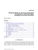
Remote Sensing and GIS Accuracy Assessment - Chapter 15 docx
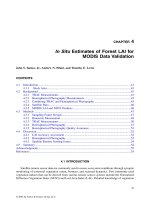
Bạn đang xem bản rút gọn của tài liệu. Xem và tải ngay bản đầy đủ của tài liệu tại đây (337.14 KB, 12 trang )
209
CHAPTER
15
The Effects of Classification Accuracy
on Landscape Indices
Guofan Shao and Wenchun Wu
CONTENTS
15.1 Introduction 209
15.2 Methods 210
15.2.1 Relative Errors of Area (REA) 211
15.3 Results 213
15.4 Discussion 214
15.5 Conclusions 217
15.6 Summary 219
Acknowledgments 219
References 219
15.1 INTRODUCTION
Remote sensing technology has advanced markedly during the past decades. Accordingly,
remote sensor data formats have evolved from image (pre-1970s) to digital formats subsequent to
the launch of Landsat (1972), resulting in a proliferation of derivative map products. The accuracy
of these products has become an integral analysis step essential to evaluate appropriate applications
(Congalton and Green, 1999). During the past three decades, accuracy assessment has become
widely applied and accepted. Although methodologies have improved, little attention has been
given to the effects of classification accuracy on the development of landscape metrics or indices.
Thematic maps derived from image classification are not always the final product from the
user’s perspective (Stehman and Czaplewski, 1998). Because all image processing or classification
inevitably introduces errors into the resultant thematic maps, any subsequent quantitative analyses
will reflect these errors (Lunetta et al., 1991). Landscape metrics are commonly derived from remote
sensing-derived LC maps (O’Neill et al., 1988; McGarigal and Marks, 1994; Frohn, 1998). Metrics
are commonly used to compare landscape configurations through time or across space, or as
independent variables in modeling linking spatial pattern and process (Gustafson, 1998). Therefore,
conclusions drawn directly or indirectly from analyzing landscape metrics contain uncertainties.
The relationships between the accuracy of LC maps and specific derived landscape metrics are
L1443_C15.fm Page 209 Saturday, June 5, 2004 10:41 AM
© 2004 by Taylor & Francis Group, LLC
210 REMOTE SENSING AND GIS ACCURACY ASSESSMENT
quite variable (i.e., metric dependent), which complicates assessment efforts (Hess, 1994; Shao et
al., 2001).
A major obstacle to assessing the accuracy of LC maps is the high cost of generating reference
data or multiple thematic maps for subsequent comparative analysis. Commonly employed solutions
include (1) selecting subsectional maps from a region (Riitters et al., 1995), (2) subdividing regional
maps into smaller maps (Cain et al., 1997), or (3) creating multiple maps using computer simulations
(Wickham et al., 1997; Yuan, 1997). Maps created using the first or second method are spatially
incompatible or incomparable, while maps created using the third method contain errors that do
not necessarily represent those found in actual LC maps. Therefore, it is necessary to create multiple
maps for a specific geographic area using different analysts or different classification methods
(Shao et al., 2001). The approach presented here represents an actual image data analysis and,
therefore, conclusions drawn from the analysis should be broadly applicable.
Past studies have focused on only a few indices. Hess and Bay (1997) made a breakthrough in
quantifying the uncertainties of adjusted diversity indices. Various statistical models have also been
developed to assess the accuracy of total area (%LAND) for individual cover types (Bauer et al.,
1978; Card, 1982; Hay, 1988; Czaplewski, 1992; Dymond, 1992; Woodcock, 1996). However, few
have used modeling to perform area calibrations (Congalton and Green, 1999). Shao et al. (2003)
derived the Relative Area Error (REA) index, which has causal relationships with area estimates
of LC categories. This study employed multiple classifications and reference maps to demonstrate
how classification accuracy affects landscape metrics. Here the overall accuracy and REA were
compared and a simple method was demonstrated to revise %LAND values using corresponding
REA index values.
15.2 METHODS
Multiple thematic maps were derived from subscenes of Landsat Thematic Mapper (TM) data
for two sites (A and B) located in central Indiana and the temperate forest zone on the eastern
Eurasian continent (at the border of China and North Korea). LC mapping was performed to
approximate a Level I classification product (Anderson et al., 1976). Site A thematic maps included
the following classes: (1) agriculture (including grassland), (2) forest (including shrubs), (3) urban,
and (4) water. The second site included only forest and nonforest (clear cuts and other open areas)
cover types. A total of 23 independent thematic maps were developed for site A. Analysts (
n
= 23)
were allowed to use any method to classify the TM imagery acquired on October 5, 1992. LC maps
were evaluated based on the overall accuracy. All the accuracies were comparable because all
assessments were performed using the same reference data set. Students performed the image
analysis, thus representing work performed by nonprofessionals (Shao et al., 2001).
Eighteen thematic maps were created for site B using a single TM data set acquired on
September 4, 1993, and a stack data set combining the 1993 data with other TM data acquired on
September 21, 1987. Training samples were acquired using three methods, including (1) computer
image interpretation, (2) field observations, and (3) and a combination of the two. Three classifi-
cation algorithms were used, including (1) the minimum distance (MD), (2) maximum likelihood
(ML), and (3) extraction and classification of homogeneous objects (ECHO). Our goal was to make
the classification process repeatable, and therefore to represent a professional work process (Wu
and Shao, 2002). Two additional maps with 94.0% and 94.5% overall accuracy that were created
with alternative approaches were also incorporated into this study.
The overall accuracy of these
maps ranged from 82.6% to 94.5% (Wu and Shao, 2002). More importantly, a reference map was
manually digitized for site B. The errors of landscape metrics of each map were computed as:
(15.1)
EIII
index map ref ref
=- ¥( ) / 100
L1443_C15.fm Page 210 Saturday, June 5, 2004 10:41 AM
© 2004 by Taylor & Francis Group, LLC
THE EFFECTS OF CLASSIFICATION ACCURACY ON LANDSCAPE INDICES 211
where
E
index
= relative errors (in percentage) of a given landscape index for a given thematic map,
I
map
= landscape index value derived from a thematic map, and
I
ref
= landscape index value derived
from a reference map.
Thematic maps were assigned to three accuracy groups based on the overall accuracy maps at
site A (
n
= 23). Landscape metrics were computed for each map with the FRAGSTATS for site A
(McGarigal and Marks, 1994) and with patch analyst (PA) for site B (Elkie et al., 1999). Nine
landscape indices were used for site A: largest patch index (LPI), patch density (PD), mean patch
size (MPS), edge density (ED), area-weighted mean shape index (AWMSI), mean nearest neighbor
distance (MNN), Shannon’s diversity index (SHDI), Simpson’s diversity index (SDI), and contagion
index (CONTAG). Thirteen landscape indices were used for site B: PD, MPS, patch size coefficient
of variance (PSCOV), patch site standard deviation (PSSD), ED, mean shape index (MSI), AWMSI,
mean patch fractal dimension (MPFD), area-weighted mean patch fractal dimension (AWMPFD),
MNN, mean proximity index (MPI), SDI, and%LAND. These landscape indices had broad repre-
sentation within the different cover categories (McGarigal and Marks, 1994).
15.2.1 Relative Errors of Area (REA)
If a thematic map
contains
n
classes or types, its accuracy can be assessed with an error matrix
(Table 15.1).
For a given patch type
k
(1
£
k
£
n
), the reference value of %LAND (LR
k
) is computed as:
(15.2)
The classification value of %LAND (LC
k
) is derived as:
(15.3)
Table 15.1 A General Presentation of an Error Matrix
Adapted from Congalton and Green (1999)
Classified
Cover Type
Reference Data
1
j
n
Total
1
f
11
f
1
j
f
1
n
f
1+
if
i
1
f
ij
f
in
f
i
+
nf
n
1
f
nj
f
nn
f
n
+
Total
f
+1
f
+
j
f
+
n
N
Note: n
= the total number of land cover types;
N
= the total
number of sampling points;
f
ij
(
i
and
j
= 1, 2, …,
n
) =
the joint frequency of observations assigned to type
i
by classification and to type
j
by reference data;
f
i
+
=
the total frequency of type
i
as derived from the clas-
sification; and
f
+
j
= the total frequency of type
j
as
derived from the reference data.
LR
f
N
f
N
ff
N
k
k
ik
i
n
ik
i
ik
n
kk
== =
+
+=
=
π
Â
Â
1
1
LC
f
N
f
N
ff
N
k
k
kj
j
n
kj
j
jk
n
kk
== -
+
+
=
=
π
Â
Â
1
1
L1443_C15.fm Page 211 Saturday, June 5, 2004 10:41 AM
© 2004 by Taylor & Francis Group, LLC
212 REMOTE SENSING AND GIS ACCURACY ASSESSMENT
Thus, the difference between
LC
k
and
LR
k
is:
(15.4)
If
LC
k
–
LR
k
= 0, there are two possibilities: classification errors are zero, or commission errors
(CE) and omission errors (OE) are the same for patch type
k
. The first possibility is normally untrue
in reality. In many situations, the second possibility is also untrue. If
CE
k
>
OE
k
,
LC
k
–
LR
k
> 0,
the value of %LAND of type
k
is overestimated; if
CE
k
<
OE
k
,
LC
k
–
LR
k
< 0, the value of %LAND
of type
k
is underestimated. Therefore, the components of
CE
k
and
OE
k
in Equation 15. 4 determine
the accuracy of %LAND for patch type
k
.
Mathematically,
CE
k
is just as follows:
CE
k
= (15.5)
OE
k
is just expressed as:
OE
k
= (6)
The balance between
CE
k
and
OE
k
indicates the absolute errors of area estimate for patch type
k
. The relative errors of area (REA) are then defined as:
(15.7)
where
f
kk
is an element of the
k-
th row and
k-
th column in an error matrix. It represents the frequency
of sample points that are correctly classified.
According to
Congalton and Green (1999), user’s accuracy of type
k
(UA
k
) can be expressed as:
(15.8)
and producer’s accuracy of type
k
(PA
k
) can be expressed as:
LC LR
ff
N
ff
N
ff
N
kk
kk
kj
j
n
ik
i
n
kj
j
jk
n
ik
i
ik
n
-=
-
=
-
=
-
++
==
=
π
=
π
ÂÂ
ÂÂ
11
11
f
kj
j
jk
n
=
π
Â
1
f
ik
i
ik
n
=
π
Â
1
REA
ff
f
k
kj
j
jk
n
ik
i
ik
n
kk
=
-
¥
=
π
=
π
ÂÂ
11
100
UA
f
f
f
f
f
ff
k
kk
k
kk
kj
j
n
kk
kk kj
j
jk
n
== =
+
+
==
π
ÂÂ
11
L1443_C15.fm Page 212 Saturday, June 5, 2004 10:41 AM
© 2004 by Taylor & Francis Group, LLC
THE EFFECTS OF CLASSIFICATION ACCURACY ON LANDSCAPE INDICES 213
(15.9)
By substituting Equation 15.8 and Equation 15.9 into Equation 15.7, it is easily derived that:
(15.10)
Thus, REA can be obtained using information on the error matrix or the user’s and producer’s
accuracy.
Under the assumption that the distribution of errors in the error matrix is representative of the
types of misclassification made in the entire area classified, it is easy to calibrate area estimates
with REA or UA and PA as follows:
(15.11)
where
A
c,k
= calibrated area in percentage for a given land cover type
k
and
A
pc,k
= precalibrated
area in percentage for a given land cover type
k
.
15.3 RESULTS
Figure 15.1 shows the means and standard deviations of nine landscape indices for three
accuracy groups. Except for PD and MPS, landscape indices had < 10% differences in their means
among three accuracy groups. The standard deviations of the landscape indices in the lowest
accuracy group are much higher than those in the higher accuracy groups. The differences in
standard deviations between the lowest accuracy group and other two accuracy groups exceeded
100%, indicating that the uncertainties were higher when classification accuracy was lower.
The statistics of classification accuracy, including the overall accuracy, producer’s accuracy,
and user’s accuracy, all have differences of < 20% among the three accuracy groups (Figure 15.2a).
The standard deviation values for overall accuracy are also about the same among the three accuracy
groups but are clearly different for producer’s accuracy and user’s accuracy (Figure 15.2b). Maps
in the lowest accuracy group have much higher variations in producer’s accuracy and user’s accuracy
than those in the other two accuracy groups.
For a few indices, such as MPDF, AWMPFD, and SDI at the landscape level, no matter what
the classification accuracy was, the errors of landscape indices were within a range of 10% (Figure
15.3). If classification accuracy was poor, the errors of some other landscape indices exceeded
100%. They include PD, PSCOV, ED, AWMSI, and MPI for entire landscapes or forest patches
(Figure 15.3 and Figure 15.4). Although no constant relationships were found between the overall
accuracy and landscape indices, maps with higher classification accuracy resulted in lower errors
for most landscape indices (Figure 15.3 and Figure 15.4). However, overall accuracy did not have
good control over the variations of landscape index errors and therefore was not a reliable predictor
for the errors of landscape indices. This was particularly true when the overall accuracy was
relatively low.
PA
f
f
f
f
f
ff
k
kk
k
kk
ik
i
n
kk
kk ik
i
ik
n
== =
+
+
==
π
ÂÂ
11
REA
UA PA
k
kk
=-
Ê
Ë
Á
ˆ
¯
˜
¥
11
100
AA
f
N
REA A
f
NUAPA
c k pc k
kk
kpck
kk
kk
,, ,
=-¥ =-¥ -
Ê
Ë
Á
ˆ
¯
˜
¥
11
100
L1443_C15.fm Page 213 Saturday, June 5, 2004 10:41 AM
© 2004 by Taylor & Francis Group, LLC
214 REMOTE SENSING AND GIS ACCURACY ASSESSMENT
The errors of %LAND have a perfect linear relationship with REA (R
2
= 0.98), but the errors
of all other indices did not show a simple relationship with REA (Figure 15.5). The REA seemed
to have a better control over landscape indices errors than did overall accuracy; the variations of
landscape index errors corresponding to REA were smaller than those corresponding to overall
accuracy (Figure 15.4 and Figure 15.5). Also, the lowest errors of landscape indices normally
occurred when REA reached zero (Figure 15.5). Both overall accuracy and REA were not reliable
indicators for explaining variations of spatially sophisticated landscape indices, such as MNN
and MPI.
The relative errors of %LAND for the forest from the 20 maps ranged from 12 to 25% before
calibration (Figure 15.6a). Based on Equation 15.11, the values of %LAND for the forest were
calibrated and resulting errors of %LAND for the forest were between 2 and 5% (Figure 15.6b),
much lower than the errors before calibration.
15.4 DISCUSSION
Methods used for image classification determine thematic maps’ classification content and
quality. Although different statistics are used for assessing the accuracy of image data classifications,
most are derived directly or indirectly from error matrices. Indices of thematic map accuracy indicate
how well image data are classified but do not tell how thematic maps correspond to a landscape’s
structure and function. This is partly because there is no effective approach to quantify classification
Figure 15.1
The mean and standard deviations for nine selected landscape indices for three accuracy groups;
1 = lowest accuracy, 2 = intermediate accuracy, 3 = highest accuracy.
123
0
5
10
15
20
25
30
35
123
Mean
0
1
2
3
4
5
6
7
8
9
10
123
Mean
0
2
4
6
8
10
12
14
16
Mean
0
2
4
6
8
10
12
14
123
Std. Dev.
0
1
2
3
4
5
6
123
Std. Dev.
0
1
2
3
4
5
6
123
Std. Dev.
Largest Patch Index
Patch Density
Mean Patch Size
0
10
20
30
40
50
60
123
Mean
0
1
2
3
4
5
6
7
8
9
10
123
Mean
0
15
30
45
60
75
90
105
120
123
Mean
0
2
4
6
8
10
12
123
Std. Dev.
0
0.2
0.4
0.6
0.8
1
1.2
1.4
1.6
1.8
2
123
Std. Dev.
0
5
10
15
20
25
30
123
Std. Dev.
Edge Density AWM Shape Index Nearest Neighbor Distance
0
0.1
0.2
0.3
0.4
0.5
0.6
0.7
0.8
0.9
1
123
Mean
0
0.1
0.2
0.3
0.4
0.5
0.6
123
Mean
0
10
20
30
40
50
60
70
123
Mean
0
0.02
0.04
0.06
0.08
0.1
0.12
0.14
0.16
12 3
Std. Dev.
0
0.02
0.04
0.06
0.08
0.1
0.12
123
Std. Dev.
0
1
2
3
4
5
6
7
123
Std. Dev.
Shannon’s Diversity Index Simpson’s Diversity Index Contagion Index
L1443_C15.fm Page 214 Tuesday, June 15, 2004 10:09 AM
© 2004 by Taylor & Francis Group, LLC
THE EFFECTS OF CLASSIFICATION ACCURACY ON LANDSCAPE INDICES 215
errors that have causal relationships with landscape function. Overall accuracy is the most frequently
used accuracy statistics, but it has limited control over the errors of landscape indices. In practice,
greater overall accuracy resulted in more controllable errors associated with landscape indices.
Only an unrealistic, 100% accurate map represents perfect source data for computing landscape
indices. For example, the overall accuracy of LC and LU maps derived from TM data for the eastern
U.S. was 81% for Anderson Level I (i.e., water, urban, barren land, forest, agricultural land, wetland,
and rangeland) and was 60% for Anderson Level II (Vogelmann et al., 2001). Such classification
accuracies are not high enough for ensuring reliable landscape index calculations.
Overall accuracy did not have a causal control over the variability of index accuracies. When
overall accuracy was relatively low, it also lost control over the difference between user’s and
producer’s accuracies. It also appeared that the uncertainties of landscape indices were more
sensitive to the variations in user’s and producer’s accuracies than to overall accuracy values alone.
REA values reflected the differences between user’s and producer’s accuracies and therefore had
a better control over the errors of landscape indices than did overall accuracy, particularly when
overall accuracy was relatively low.
Because REA is derived for assessing the accuracy of %LAND, this index alone can be
used to predict the errors of %LAND. The linear relationship with REA and the area of forested
land verifies the reliability of such predictions with REA. While the overall accuracy is approx-
imately the average of user’s and producer’s accuracy, REA reveals the differences between
user’s and producer’s accuracy. Therefore, the overall accuracy and REA explained different
aspects of classification accuracy. Although the lowest errors of landscape indices often occur
when REA is near zero, variations in the errors of landscape indices still existed. When REA
and the overall accuracy were used together, the errors of landscape indices were better predicted
Figure 15.2
The mean (a) and standard deviation (b) values for overall and individual classification accuracies;
LA = lowest accuracy, IA = intermediate accuracy, HA = highest accuracy.
0
20
40
60
80
100
120
LA Group
IA Group
HA Group
LA Group
IA Group
HA Group
0
5
10
15
20
25
(b)
(a)
Landscape Urban Forest Water Urban Agriculture Forest Water
User’s
Accuracy
User’s
Accuracy
Producer’s
Accuracy
Producer’s
Accuracy
Overall
Accuracy
Overall
Accuracy
Agriculture
Landscape Urban Forest Water Urban Agriculture Forest WaterAgriculture
L1443_C15.fm Page 215 Tuesday, June 15, 2004 10:09 AM
© 2004 by Taylor & Francis Group, LLC
216 REMOTE SENSING AND GIS ACCURACY ASSESSMENT
(the greater overall accuracy, the smaller REA). However, overall accuracy and REA explained
some aspects of classification errors but did not explain other possible sources of classification
errors (e.g., the spatial distributions of misclassifications). Therefore, these accuracy measures
alone were not adequate to assess the accuracy of the MNN and MPI, which have particularly
strong spatial features.
The variations of landscape index errors were different among different landscape indices. For
example, the errors of MPDF, AWMPFD, and SDI at the landscape level were within a range of
10%, whereas the errors of PD, PSCOV, ED, AWMSI, and MPI for entire landscapes or forest
patches exceeded 100%. The former group of landscape indices was not as sensitive to image data
classification and the errors of these landscape indices were not controlled by classification accuracy
measures. Landscape indices in this group were unreliable despite the image classification accuracy
values. The latter group of landscape indices was sensitive to image data classifications, and
therefore a small difference in classification accuracy resulted in a large difference in landscape
index values. In this case, classification accuracy was always superior when accuracy-sensitive
landscape indices were used. Intermediate indices exhibited intermediate sensitivity to image data
classifications. The rule of higher overall accuracy and smaller absolute values of REA was
particularly applicable to this intermediate group. Further systematic studies are needed to determine
which landscape index belongs to these sensitive groups.
Figure 15.3
The relative errors of 12 selected landscape indices for the landscape (y-axis) against the overall
accuracy (x-axis).
SDI
−15
−10
−5
0
5
82 84 86 88 90 92 94 96
MPI
-50
0
50
100
150
200
82 84 86 88 90 92 94 96
MNN
−50
−40
−30
−20
−10
0
82 84 86 88 90 92 94 96
AWMPFD
2
4
6
8
10
82 84 86 88 90 92 94 96
MPFD
−7
−6
−5
−4
−3
−2
82 84 86 88 90 92 94 96
MSI
−45
−40
−35
−30
−25
−20
−15
82 84 86 88 90 92 94 96
ED
0
30
60
90
120
150
82 84 86 88 90 92 94 96
PSSD
−100
−90
−80
−70
−60
−50
−40
−30
82 84 86 88 90 92 94 96
PSCOV
0
100
200
300
400
500
82 84 86 88 90 92 94 96
MPS
−100
−90
−80
−70
−60
−50
82 84 86 88 90 92 94 96
PD
0
200
400
600
800
1000
1200
1400
1600
82 84 86 88 90 92 94 96
AWMSI
0
20
40
60
80
100
120
140
82 84 86 88 90 92 94 96
L1443_C15.fm Page 216 Saturday, June 5, 2004 10:41 AM
© 2004 by Taylor & Francis Group, LLC
THE EFFECTS OF CLASSIFICATION ACCURACY ON LANDSCAPE INDICES 217
15.5 CONCLUSIONS
The uncertainties or errors associated with landscape indices vary in their responses to image
data classifications. Also, the existing statistical methods for assessing classification accuracy have
different controls relative to the uncertainties or errors of landscape indices. Assessing accuracy of
landscape indices requires combined knowledge of the overall accuracy (means of user’s accuracy
and producer’s accuracy) and the REA (differences between user’s accuracy and producer’s accu-
racy). To reliably characterize landscape conditions using landscape indices, our results indicate it
is necessary to use maps with high overall accuracy and low absolute REA. The selections of
landscape indices are also important because different landscape indices have different sensitivities
to image data classifications. Based on commonly achievable levels of classification accuracy, the
magnitudes of errors associated with landscape indices can be higher than the values of landscape
indices. Comparisons between different thematic maps should consider these errors. Assuming that
the distribution of errors identified by the error matrix is representative of the misclassifications
across the area of interest, the total land area of different class categories can be revised with REA
and the errors of this landscape index can be lowered. Revised values of %LAND should be used
when quantifying landscape conditions.
Figure 15.4
The relative errors of 12 selected landscape indices for forest class (y-axis) against the overall
accuracy (x-axis).
%LAND
−20
−10
0
10
20
30
82 84 86 88 90 92 94 96
MPI
−200
0
200
400
600
800
1000
82 84 86 88 90 92 94 96
MNN
−20
−10
0
10
20
30
82 84 86 88 90 92 94 96
AWMPFD
0
5
10
15
20
82 84 86 88 90 92 94 96
MPFD
−8
−6
−4
−2
0
82 84 86 88 90 92 94 96
MSI
−45
−40
−35
−30
−25
−20
−15
82 84 86 88 90 92 94 96
ED
0
30
60
90
120
150
82 84 86 88 90 92 94 96
PSSD
−100
−50
0
50
100
150
82 84 86 88 90 92 94 96
PSCOV
0
100
200
300
400
500
82 84 86 88 90 92 94 96
MPS
−100
−80
−60
−40
−20
0
82 84 86 88 90 92 94 96
PD
0
200
400
600
800
1000
82 84 86 88 90 92 94 96
AWMSI
0
100
200
300
400
500
82 84 86 88 90 92 94 96
L1443_C15.fm Page 217 Saturday, June 5, 2004 10:41 AM
© 2004 by Taylor & Francis Group, LLC
218 REMOTE SENSING AND GIS ACCURACY ASSESSMENT
Figure 15.5
The relative errors of 12 selected landscape indices for forest class (y-axis) against the REA (x-axis).
Figure 15.6
A comparison of %LAND errors for for-
est class among thematic maps (
n
= 20)
before calibrations (a) and after calibra-
tions (b).
MPI
−200
0
200
400
600
800
1000
−20.00 −10.00
0.00 10.00 20.00
MNN
−20
−10
0
10
20
30
−20.00 −10.00
0.00 10.00 20.00
MSI
−45
−40
−35
−30
−25
−20
−15
−20.00 −10.00 0.00 10.00 20.00
AWMPFD
0
5
10
15
20
-20.00
−10.00
0.00 10.00 20.00
%LAND
−20
−10
0
10
20
30
−20.00 −10.00
0.00 10.00 20.00
ED
0
30
60
90
120
150
−20.00 −10.00 0.00 10.00 20.00
MPFD
−8
−6
−4
−2
0
−20.00 −10.00
0.00 10.00 20.00
PSSD
−100
−50
0
50
100
150
−20.00 −10.00 0.00 10.00 20.00
PSCOV
0
100
200
300
400
500
−20.00 −10.00 0.00 0.00 20.00
MPS
−100
−80
−60
−40
−20
0
−20.00
−10.00 0.00 10.00 20.00
PD
0
200
400
600
800
1000
−20.00 −10.00
0.00 10.00 20.00
−20.00 −10.00
0.00 10.00 20.00
AWMSI
0
100
200
300
400
500
−20
−10
0
10
20
30
−20
−10
0
10
20
30
(a)
(b)
L1443_C15.fm Page 218 Saturday, June 5, 2004 10:41 AM
© 2004 by Taylor & Francis Group, LLC
THE EFFECTS OF CLASSIFICATION ACCURACY ON LANDSCAPE INDICES 219
15.6 SUMMARY
A total of 43 LC maps from two study sites were used to demonstrate the effects of classification
accuracy on the uncertainties or errors of 15 selected landscape indices. The measures of classifi-
cation accuracy used in this study were the overall accuracy and REA. The REA was defined as
the difference between the reciprocals of user’s accuracy and producer’s accuracy. Under variable
levels of classification accuracy, different landscape indices had different uncertainties or errors.
These variations or errors were explained by both the overall accuracy and REA. Thematic maps
with relatively high overall accuracy and low absolute REA ensured lower uncertainties or errors
of at least several landscape indices. For landscape indices that were sensitive to classification
accuracy, a small increase in classification accuracy resulted in a large increase in their accuracy.
Assuming that the error matrix truly represents misclassification errors, the total areas of different
class categories can be calibrated using the REA index and the accuracy of quantifying or comparing
relative landscape characteristics can be increased.
ACKNOWLEDGMENTS
Thematic LC maps used in this study were partially provided by 23 students from a remote
sensing class offered at Purdue University in 1999. The Cooperative Ecological Research Program
in cooperation with the China Academy of Sciences and the German Department of Science and
Technology provided the TM data used in this study. The authors would like to thank the book
editors and anonymous reviewers for their insightful comments and suggestions on the manuscript.
REFERENCES
Anderson, J.R., E.E. Hardy, J.T. Toach, and R.E. Witmer, A Land Use and Land Cover Classification System
for Use with Remote Sensor Data, U.S. Geological Survey professional paper 964, U.S. Government
Printing Office, Washington, DC, 1976.
Bauer, M.E., M.M. Hixson, B.J. Davis, and J.B. Etheridge, Area estimation of crops by digital analysis of
Landsat data,
Photogram. Eng. Remote Sens.,
44, 1033–1043, 1978.
Cain, D.H., K. Riitters, and K. Orvis, A multi-scale analysis of landscape statistics,
Landsc. Ecol.,
12, 199–212,
1997.
Card, D.H., Using map categorical marginal frequencies to improve estimates of thematic map accuracy,
Photogram. Eng. Remote Sens.,
48, 431–439, 1982.
Congalton, R.G. and K. Green,
Assessing the Accuracy of Remotely Sensed Data: Principles and Practices
,
Lewis, Boca Raton, FL, 1999.
Czaplewski, R.L., Misclassification bias in areal estimates,
Photogram. Eng. Remote Sens
., 58, 189–192, 1992.
Dymond, J.R., How accurately do image classifier estimate area?
Int. J. Remote Sens.,
13, 1735–1342, 1992.
Elkie, P., R. Rempel, and A. Carr,
Patch Analyst User’s Manual, Ontario Ministry of Natural Resources,
Northwest Science & Technology,
Thunder Bay, Ontario, Tm-002, 1999.
Frohn, R.C.,
Remote Sensing for Landscape Ecology: New Metric Indicators for Monitoring, Modeling, and
Assessment of Ecosystems
, Lewis, Boca Raton, FL, 1998.
Gustafson, E.J., Quantifying landscape spatial pattern: what is the state of the art?
Ecosystems
, 1, 143–156, 1998.
Hay, A.M., The derivation of global estimates from a confusion matrix,
Int. J. Remote Sens
., 9, 1395–1398,
1988.
Hess, G.R., Pattern and error in landscape ecology: a commentary,
Landsc. Ecol.,
9, 3–5, 1994.
Hess, G.R. and J.M. Bay, Generating confidence intervals for composition-based landscape indexes,
Landsc.
Ecol.,
12, 309–320, 1997.
Lunetta, R.S., R.G. Congalton, L.F. Fenstermaker, J.R. Jensen, K.C. McGwire, and L.R. Tinney, Remote
sensing and geographic information system data integration: error sources and research issues,
Pho-
togram. Eng. Remote Sens.,
57, 677–687, 1991.
L1443_C15.fm Page 219 Saturday, June 5, 2004 10:41 AM
© 2004 by Taylor & Francis Group, LLC
220 REMOTE SENSING AND GIS ACCURACY ASSESSMENT
McGarigal, K. and B.J. Marks, FRAGSTATS: Spatial Patterns Analysis Program for Quantifying Landscape
Structure, unpublished software, USDA Forest Service, Oregon State University, 1994.
O’Neill, R.V., J.R. Krummel, R.H. Gardner, G. Sugihara, B. Jackson, D.L. DeAngelis, B.T. Milne, M.G.
Turner, B. Zygnut, S.W. Christensen, V.H. Dale, and R.L. Graham, Indices of landscape pattern,
Landsc. Ecol.,
1, 152–162, 1988.
Riitters, K.H., R.V. O’Neill, C.T. Hunsaker, J.D. Wickham, D.H. Yankee, S.P. Timmins, K.B. Jones, and B.L.
Jackson, A factor analysis of landscape pattern and structure metrics,
Landsc. Ecol.,
10, 23–39, 1995.
Shao, G., D. Liu, and G. Zhao, Relationships of image classification accuracy and variation of landscape
statistics,
Can. J. Remote Sens.,
27, 33–43, 2001.
Shao, G., W. Wu, G. Wu, X. Zhou, and J. Wu, An explicit index for assessing the accurace of cover class
areas,
Photogram. Eng. Remote Sens.
, 69(8), 907–913, 2003.
Stehman, S.V. and R.L. Czaplewski, Design and analysis for thematic map accuracy assessment: fundamental
principles,
Remote Sens. Environ.,
64, 331–344, 1998.
Vogelmann, J.E., M.H. Stephen, L. Yang, C.R. Clarson, B.K. Wylie, and N. Van Driel, Completion of the
1990s national land cover data set for the conterminous United States from Landsat Thematic Mapper
data and ancillary data sources,
Photogram. Eng. Remote Sens.,
67, 650–662, 2001.
Wickham, J.D., R.V. O’Neill, K.H. Riitters, T.G. Wade, and K.B. Jones, Sensitivity of selected landscape
pattern metrics to landcover misclassification and differences in landcover composition,
Photogram.
Eng. Remote Sens.,
63, 397–402, 1997.
Wookcock, C.E., On the roles and goals for map accuracy assessment: a remote sensing perspective, in
Proceedings of the 2nd International Symposium on Spatial Accuracy Assessment in Natural Resources
and Environmental Sciences, Fort Collins, CO, 1996, USDA Forest Service Rocky Mountain Forest
and Range Experiment Station, Technical Report RM-GTR-277, 1996, pp. 535–540.
Wu, W. and G. Shao, Optimal combinations of data, classifiers, and sampling methods for accurate charac-
terizations of deforestation
, Can. J. Remote Sens.,
28, 601–609, 2002.
Yuan, D., A simulation of three marginal area estimates for image classification,
Photogram. Eng. Remote
Sens
., 63, 385–392, 1997.
L1443_C15.fm Page 220 Saturday, June 5, 2004 10:41 AM
© 2004 by Taylor & Francis Group, LLC