New Approaches in Automation and Robotics part 5 docx
Bạn đang xem bản rút gọn của tài liệu. Xem và tải ngay bản đầy đủ của tài liệu tại đây (1.02 MB, 30 trang )
Bilinear Time Series in Signal Analysis
113
2. Bilinear time series models
Large amount of dynamical systems may be described with set of conservation equations in
the following form:
1
()
() () ()(),
m
kk
k
dt
tt utt
dt
=
+=+
∑
x
Ax Bu N x (7)
where the last term creates the bilinear part of the equation. Bilinear equations are the
natural way of description of a number of chemical technological processes like decantation,
distillation, and extraction, as well as biomedical systems, e.g. (Mohler, 1999), (Nise, 2000).
Though the nature of many processes is bilinear, identification of the model (7) can be
difficult, at least because some of the state or input variables may be immeasurable. This is
the case of many biological or biomedical processes. Often, the discrete set of the output
observation {y
i
}, for i=1,…,n, is the only information on the considered process. In such
cases bilinear time series model (8), which explains relation between the set of the output
data only, may be considered.
11
1
1
() ()
L
K
ii ikil
kl
l
k
Az y Cz e e yβ
−−
=+
−−
=
=
∑
∑
(8)
Bilinear time series models have been mentioned in control engineering since early
seventieth. Schetzen Theorem (Schetzen, 1980) states, that any stable time variant process
may be modeled as time invariant bilinear time series. General structure of bilinear time
series model (8) is complex enough to make its analysis very difficult. Therefore, in practise
the particular model structures are being analysed.
Stochastic processes are completely characterized by their probabilistic structure, i.e.
probability or probability density p(y) (e.g. Therrien, 1992). However, in practice,
probabilistic structure of a considered system is unknown and, therefore, the system
analysis is performed on the ground of its statistical moments. The moments for any
stochastic process with any probabilistic density p(y) are expressed as:
()
}{
r
r
y
i
M
Ey= (9)
where E is an operator of expected value :
{} ()
x
Ey ypy μ==
∑
. (10)
Central moments are:
()
'
}{( )
r
r
y
MEy
i
μ= − (11)
When the structure of particular bilinear model is simple, the moments and the central
moments may be analytically calculated based on the process equation, and the moments’
definitions (9), (11). Elementary bilinear time series models, considered in this chapter, in
dependence on their structures, are classified as sub diagonal or diagonal.
New Approaches in Automation and Robotics
114
2.1 Sub diagonal elementary bilinear time series EB(k,l)
When the structure k,l of elementary bilinear time series model EB(k,l) satisfy relation kl< ,
the model (12) is named sub diagonal.
,
ii klikil
y
eeyβ
−−
=+ (12)
The model is characterized by two parameters,
kl
β and
2
e
m , related to each other. It may be
proven, (e.g. Tong, 1993) that the model (12) is stable when
2(2)
| |1
kl e
mβ < , and is invertible
when
2(2)
||0.5
kl e
mβ < . Time series invertibility means that for a stable time series
1,1
( , , , , , )
iiiiki il
y
fee e y y
−−− −
= (13)
operation of inversion
1,1
( , , , , , )
iiikii il
efe eyy y
−
−−−
=
(14)
is stable. The moments and the central moments of EB(k,l) may be analytically calculated
based on the process equation (12), and the moments' definitions (9), (11). Relations between
moments and parameters are given in the table 1. The variance
(2)
(0)
y
M of EB(k,l) is bounded
when:
2(2)
| |1.
kl e
mβ < (15)
The fourth moment
(4)
(0,0,0)
y
M of EB(k,l) is bounded when:
4(4)
| |1
kl e
mβ < (16)
Irrespective of the probabilistic density of
i
e , sub diagonal EB(k,l) is non-Gaussian and
uncorrelated. Gaussian equivalent of the sub diagonal EB(k,l) with a bounded variance is a
Gaussian white noise with the first and the second moments the same as the respective
moments of the EB(k,l). Comparison of an EB(2,4) time series and its Gaussian equivalent is
shown in the Fig.(1).
Table 1. Relation between moments and EB(k,l) parameters
Moments Formulae
(1)
y
M
0
(2)
(0)
y
M
(2)
(0)
y
Mm>
(2)
2(2)
1
e
kl e
m
mβ−
0
(3)
(0,0)
y
M
(3)
12
(,)
y
M
lkll≠≠
(3)
(,)
y
M
kl
0
0
(2) (2)
(0)
kl e y
mMβ
(4)
(0,0,0)
y
M
(4) 2 (2) 2 (2)
4(4)
6( ) (0)
1
ekley
kl e
mmM
m
β
β
+
−
Bilinear Time Series in Signal Analysis
115
Fig. 1. Comparison of the estimated moments of EB(2,4) and an equivalent white noise
2.2 Diagonal elementary bilinear time series EB(k,k)
Elementary diagonal bilinear time series model, EB(k,k) has the following structure:
.
i i kkik ik
ye eyβ
−−
= + (17)
Properties of the model depend on two parameters,
kk
β
and
(2)
e
m , related to each other.
Stability and invertibility conditions for EB(k,k) are the same as for sub diagonal EB(k,l) time
series model. Having known the process equation (17) and the moments' definitions (9) and
(11), moments and central moments of the EB(k,k)may be analytically calculated as functions
of model parameters. Though EB(k,l) and EB(k,l) with respect to model equation are similar
to each other, their statistical characteristics are significantly different. Relation between
New Approaches in Automation and Robotics
116
succeeding moments and model parameters are given in the table 2. An example of a single
realization of EB(5,5) series as well as its sampled moments is shown in the the Fig. 2.
Table 2. Relations between moments and EB(k,k) parameters
Fig. 2. EB(5,5) sequence and its characteristics
Moments Formulae
(1)
y
M
(2)
kk e
mβ
(2)
(0)
y
M
(2)
()
y
M
mk≠
(2)
()
y
M
k
(2) 2 (4) (2) 2
2(2)
(())
1
ekke e
kk e
mmm
m
β
β
+−
−
(
)
2
2(2)
kk e
mβ
(
)
2
2(2)
2
kk e
mβ
(3)
(0,0)
y
M
(3)
(, )
y
M
kl k<
(3)
(,)
y
M
kk
(3)
(, )
y
M
kl k>
(3)
(,2)
y
M
kk
(6) 2 (2) (6) 2 (4) 2
2(2)2 3
2(2)
3( ))
3( )
1
ekkee kke
kk e kk
kk e
mmm m
m
m
ββ
ββ
β
−+
+
−
(
)
3
3(2)
2
kk e
mβ
3(2)(4)
(4)
2(2)
3
1
kk e e
kk e
kk e
mm
m
m
β
β
β
+
−
(
)
3
3(2)
2
kk e
mβ
(
)
3
3(2)
4
kk e
mβ
Bilinear Time Series in Signal Analysis
117
Diagonal EB(k,k) time series {}
i
y
has a non-zero mean value, equal to
(1)
y
M
. Deviation from
the mean
(2)
ii
y
zyM=− is a non-Gaussian time series. A Gaussian equivalent of
i
z is a
MA(k) series:
iikik
zwcw
−
=+ (18)
where
i
w
is a Gaussian white noise series. Values of
k
c
and
(2)
w
m can be calculated from the
set of equations (19):
(2) 2 (2) 4 (2) 2
(2) 2
2(2)
2(2)2 (2)
(1 ( ) )
(1 )
1
( )
ekkekke
wk
kk e
kk e k w
mmm
mc
m
mcm
ββ
β
β
++
=+
−
=
(19)
3. Identification of EB(k,l) models
Under assumption that the model EB(k,l) is identifiable, and that the model structure is
known, methods of estimation of the model parameters are similar to the methods of
estimation of linear model parameters. The similarity stems from that the bilinear model
structure, though nonlinear in
i
e and
i
y
, is linear in parameter
kl
β . A number of estimation
methods originate from minimization of a squared prediction error (20). Three of them,
which are frequently applied in estimation of bilinear model parameters, will be discussed
in the section 3.1.
|1
ˆ
ii
ii
yyε
−
=− (20)
Moments’ methods are an alternative way of parameters’ estimation. Model parameters are
calculated on the base of estimated stochastic moments (Tang & Mohler, 1988). Moments’
methods are seldom applied, because hardly ever analytical formulae connecting moments
and model's parameters are known. For elementary bilinear time series models the formulae
were derived, (see table 1, table 2) and therefore, method of moments and generalized
method of moments, discussed in section 3.2, may be implemented to estimate elementary
bilinear models parameters.
3.1 Methods originated from minimization of the squared prediction error
Methods that originate from minimization of the squared prediction error (20) calculate
model parameters by optimization of a criterion
2
()
i
J ε , being a function of the squared
prediction error. In this section the following methods are discussed:
− minimization of sum of squares of prediction error,
− maximum likelihood,
− repeated residuum.
a) Minimization of the sum of squares of prediction error
Minimization of the sum of squares of prediction error is one of the simplest and the most
frequently used methods for time series model identification. Unfortunately, the method is
sensitive to any anomaly in data set applied in model identification (Dai & Sinha, 1989).
Generally, filtration of the large data deviation from the normal or common course of time
New Approaches in Automation and Robotics
118
series (removing outliers) precedes the model identification. However, filtration cannot be
applied to the bilinear time series, for which sudden and unexpected peaks of data follows
from the bilinear process nature, and should not be removed from the data set used for
identification. Therefore, the basic LS algorithm cannot be applied to elementary bilinear
model identification and should be replaced by a modified LS algorithm, resistant to
anomalies. Dai and Sinha proposed robust recursive version (RLS) of LS algorithm, where
kl
β parameter of the model EB(k,l) is calculated in the following way:
(
)
,,1 ,1
-1
2
1
22
1
-1
2
1
1
kli kli i i i kli
ii
i
iii
ii
ii
iiii
bb kyb
P
k
p
P
PP
p
α
αα
−−
−
−
−
=+−Φ
Φ
=
+Φ
⎛⎞
Φ
⎟
⎜
⎟
=−
⎜
⎟
⎜
⎟
⎟
⎜
+Φ
⎝⎠
(21)
where:
−
,kl i
b evaluation of model parameter
kl
β calculated in i-th iteration,
−
ˆ
iikil
wy
−−
Φ= generalized input,
−
,1
ˆ
iiikli
wy b
−
=−Φ one step ahead prediction error,
−
i
α
coefficient that depends upon the prediction error as follows:
ˆ
()
ˆ
for
ˆ
ˆ
1 for
i tresh
i tresh
i
i
i tresh
sign w y
wy
w
wy
α
⎧
⎪
⎪
>
⎪
⎪
=
⎨
⎪
⎪
≤
⎪
⎪
⎩
tresh
y a threshold value
b) Maximum likelihood
Maximum likelihood method was first applied to bilinear model identification by Priestley
(Priestley, 1980) then Subba (Subba, 1981), and others e.g. (Brunner & Hess, 1995). In this
method, elementary bilinear model EB(k,l) is represented as a function of two parameters
model
(, )
kl i k
yby
−
:
model
kl i k i l
y
by w
−−
= (22)
where
i
w is an innovation series, equivalent to the model errors:
-
mode
-(,).
ii klik
l
wyy by= (23)
Likelihood is defined as:
(2) (2)
1
(, ) (, ;)
N
kl w kl w i
i
LLbm fbmw
=
==
∏
(24)
Maximization of L is equivalent to minimization of -l=-ln(L):
(2) (2)
1
(, ) ln((, ;))
N
kl w kl w i
i
lb m
f
bm w
=
−=−
∑
(25)
Bilinear Time Series in Signal Analysis
119
Assuming that
i
w is a Gaussian series with the mean value equal to zero, and the variance
equal to
(2)
w
m , negative logarithm likelihood -ln(L) is:
2
(2) (2)
-1 1
(2)
1
-ln( ) - ( , , , | , ) ln(2 ) .
22
N
i
NN klw w
i
w
Nw
Llww wbm m
m
π
=
==+
∑
(26)
Having assumed initial values
,0kl
b and
(2)
0w
m , parameters
kl
b and
(2)
w
m are calculated by
minimization of (26). Solution is obtained iteratively, using e.g. Newton-Raphson method.
Essential difficulty lies in the fact that
i
w is immeasurable and, in each iteration, should be
calculated as:
,-1 - -
-
iikliikil
wybwy= (27)
Obtained estimates of EB(k,l) parameters are asymptotically unbiased if
i
w is Gaussian
(Kramer & Rosenblatt, 1993). For other distributions, Gaussian approximation of the
probability density function
mode
((,))
iklik
l
fy y b y
−
−
causes that the estimated parameters are
biased.
c) Repeated residuum method
Alternative estimation method, named repeated residuum method, is proposed in (Priestley,
1980). Implemented to identification of elementary bilinear models, the method may be
presented as the following sequence of steps:
1.
Model EB(k,l) is expressed as:
-
(1 )
k
ii klil
y
wb
y
D=+ (28)
or equivalently:
-
1
i
i
k
kl i l
y
w
b
y
D
=
+
(29)
2.
Assuming
kl
b
small, the (29) may be approximated by:
(1- ) - .
k
i klil i i klilik
wb
y
D
yy
b
yy
== (30)
Presuming
i
w is an identification error, an initial estimate
,0kl
b of the parameter
kl
b can
be evaluated from the (30), with the use of e.g. LS method.
3.
Next, starting from
,0kl
b
and
0
0w =
, succeeding
i
w
can be calculated iteratively:
,0
for , 1, , .
iiklikil
wybwy ikk N
−−
=− = + (31)
4.
Having known
i
y
and
i
w for i=k, N, an improved estimate
kl
b that minimizes the
following sum of squared errors (32) may be calculated.
2
() (- ).
N
kl i kl i k i l
ik
Vb y bw y
=
=
∑
(32)
5.
The steps 3 and 4 are repeated until the estimate achieves an established value.
New Approaches in Automation and Robotics
120
3.2 Moments method
With respect to the group of methods that originate from the minimization of the squared
prediction error, a precise forms of estimation algorithms can be formulated. On the
contrary, for moments method a general idea may be characterized only, and the details
depend on a model type and a model structure. Moments method MM consists of two
stages:
Stage 1: Under the assumption that the model structure is the same as the process structure,
moments and central moments
()r
y
M
are presented as a function of process parameters
Θ
:
()
()
r
y
Mf=Θ (33)
If it is possible, the moments are chosen such that the set of equations (33) has an unique
solution.
Stage 2: In (33) the moments
()r
y
M
are replaced with their evaluation
()
ˆ
r
y
M
, estimated on the
base of available data set
i
y
.
()
ˆ
()
r
y
Mf=Θ (34)
The set of equations (34) is then solved according to the parameters
Θ . Taking into
consideration particular relation between moments and parameters for elementary bilinear
models, MM estimation algorithm in a simple and a generalized version can be proposed.
MM – simple version
It is assumed that
i
w
is a stochastic series, symmetrical distributed around zero, and that
the even moments
(2 )r
w
m satisfy the following relations:
(2 ) (2)
2
( ) for 1,2,3
rr
wrw
mkm r== (35)
Identification of EB(k,l) consists of identification of the model structure (k,l), and estimation
of the parameters
kl
b and
(2)
w
m . Identification algorithm is presented below as the sequence
of steps:
1.
Data analysis:
a.
On the base of data set
{
}
i
y
for i=1, ,N, estimate the following moments:
(1) (2) (3) (4)
12 12
ˆˆ ˆ ˆ
; ( ) for 0,1,2 ; ( , ) for , 0,1,2 ; (0,0,0)
yy y y
MMm m Mll ll M==
b.
Find the values of
1
0l ≠ and
2
0l ≠ (
12
ll≤ ), for which the absolute value of
the third moment
(3)
12
ˆ
(,)
y
M
ll is maximal.
2.
Structure identification:
a. If
12
, lkll==then subdiagonal model EB(k,l) should be chosen.
b. If
12
, lklk== then diagonal model EB(k,k) should be chosen
3.
Checking system identifiability condition:
If the model EB(k,l) was chosen, than:
a. Calculate an index
(3) 2
y
3
(2) 3
y
ˆ
(M ( , ))
W=
ˆ
(M (0))
kl
(36)
Bilinear Time Series in Signal Analysis
121
b. If
3
W <0.25 it is impossible to find a bilinear model EB(k,l) that has the same
statistical characteristics as the considered process. Nonlinear identification
procedure should be stopped. In such case either linear model may be assumed, or
another non-linear model should be proposed.
If the model EB(k,k) was chosen, than:
a. Calculate an index
(3)
y
4
(2) (2)
yy
ˆ
M(,)
W=
ˆˆ
M(0)M()
kk
k
(37)
b. If
4
3
2
W
ε−<, where ε is an assumed accuracy, then the model input may be
assumed Gaussian.
i.
Calculate an index
(3) (2)
yy
5
(2) (3)
yy
ˆˆ
M(,)M()
W=
ˆˆ
M(0)M(0,0)
kk k
(38)
ii. If
5
0.23W <
, than the model EB (k,k) with the Gaussian input may be
applied. If not than linear model MA(k) should be taken into account.
c. If
4
3
2
W
ε−≥than the model input
i
w cannot be Gaussian.
4.
Estimation of model parameters :
a. When the model EB(k,l) was chosen in the step 2:
i. Find the solutions
12
,xx of the equation:
3
(1- ),Wxx= (39)
where
2(2)
kl w
xbm=
ii. For each of the solutions
12
,xx calculate the model parameters from the
following equations:
(2) (2)
2
(2)
ˆ
(0)(1 - ),
wy
kl
w
mM x
x
b
m
=
=
(40)
iii. In general, the model EB(k,l) is not parametric identifiable, i.e. there is no
unique solution of the equation (39) and (40). Decision on the the final model
parameters should be taken in dependance on model's destination. Models
applied for control and prediction should be stable and invertible. Models
used for simulation should be stable but do not have to be invertible.
b. When in the step 2 the model EB (k,k) is chosen:
New Approaches in Automation and Robotics
122
i. If
4
3
2
W
ε−≥ then
44
44 4
k-W 2
x= ,
W2( 1)2kk−−
where:
4
44
232
for <3:
22
k
kW<<
,
4
44
32 2
for >3:
22
k
kW<<
.
ii. If
4
3
2
W ≈ , i.e.
i
w is Gaussian, then the folloving equation have to be solved:
5
6(1- )
32 22^2
xx
W
xx
=
++
Because the model EB(k,k) with the Gaussian input is not parametric
identifiable, the final model should be chosen according to its destination,
taking into account the same circustances as in the paragraph a) -iii.
MM generalized version:
Generalized moments method (GMM) (Gourieroux et al., 1996) (Bond et al., 2001), (Faff &
Gray 2006), is a numerical method in which model parameters are calculated by
minimization of the following index:
2
1
(,),
J
ki
j
Ify
=
=Θ
∑
(41)
where:
Θ vector of parameters,
(,)
ji
fyΘ a function of data ()
y
i and parameters Θ , for which:
{
}
00
, 0 when =
i
EyΘ= ΘΘ (42)
0
Θ vector of parameters minimizing the index I.
Function ( , )
ji
fyΘ for j=1,2, ,J is defined as a difference between analytical moment
()
()
k
y
M Θ dependant upon the parameters Θ , and the evaluation
()
ˆ
k
y
M
calculated on the base
of
i
y for i=1, ,N. The number J of considered moments depends on the model being
identified.
Identification of the subdiagonal, elementary bilinear model EB(k,l) makes use of the four
moments. Functions
j
f
, for j=1, ,4 are defined in the following way:
(2) (2)
1
(3) (3)
2
(4) (4)
3
(2) (2)
4
ˆ
(,) (0)- (0)
ˆ
( , ) ( ,)- ( ,)
ˆ
( , ) (0,0,0)- (0,0,0)
ˆ
(,) -
iyy
iy y
iy y
iww
fy M M
fy M kl M kl
fy M M
fy m m
Θ=
Θ=
Θ=
Θ=
Bilinear Time Series in Signal Analysis
123
Diagonal model EB(k,k) is identified on the base of three moments. The functions
j
f
for
j=1, ,6 are:
(1) (1)
1
(2) (2)
2
(2) (2)
3
(3) (3)
4
(3) (3)
5
(2) (2)
6
ˆ
(,) -
ˆ
(,) (0)- (0)
ˆ
(,) ()- ()
ˆ
( , ) (0,0)- (0,0)
ˆ
(,) (,)- (,)
ˆ
(,) -
iyy
iyy
iyy
iy y
iy y
iww
fy M M
fy M M
fy MkMk
fy M M
f
yMkkMkk
fy m m
Θ=
Θ=
Θ=
Θ=
Θ=
Θ=
For elementary bilinear models vector of parameters contains two elements:
(2)
and
wkl
mb.
The parameters are calculated by minimization of the index (41), using e.g. nonlinear least
squares method. It is assumed that starting point
(2)
0,00
,
kl w
bm
⎡
⎤
Θ=
⎢
⎥
⎣
⎦
is a solution obtained with
the use of the simple method of moments. Minimum of the index I may be searched
assuming that the parameters
kl
b and
(2)
w
m are constrained. The constrains result from the
following attributes:
− The variance
(2)
w
m of the model input should be positive and less than the output
variance, hence:
(2) (2)
0,
wy
mm<< (43)
− The model should be stable, hence:
2(2)
1
kl w
bm < (44)
3.3 Examples
The methods discussed above were applied to elementary bilinear time series identification
under the following conditions:
1.
Elementary diagonal and subdiagonal time series were identified.
2.
Distribution of the white noise
i
w was assumed:
• Gaussian,
• even
with the zero mean and the variance
(2)
1
w
m = .
3.
All considered processes were invertible, i.e. the parameters satisfied the following
condition:
2(2)
0.5
kl w
bm < (Tong, 1993).
4.
Identification was performed for 200 different realizations of the time series consisted of
1000 data.
5.
For generalized moments method:
− Minimization of the performance index was carried out with the constrains:
(2) (2)
(2) (2)
-0.5 0.5
ˆ
0
kl
yy
wy
b
mm
mm
<<
<<
New Approaches in Automation and Robotics
124
−
Starting point was calculated using simple moments method.
Result of conducted investigation may be summarized as follows:
1. Not every invertible elementary bilinear process is identifiable.
2. Correct identification results were obtained for processes, for which
0.4
kl
β ≤ , what is
equivalent to:
2(2)
0.16
kl w
mβ ≤ .
3. When
2(2)
0.16
kl w
mβ > number of process realization, for which elementary bilinear model
cannot be identified grows with the growth of
2(2)
kl w
mβ .
4. When
0.4
kl
β ≤ all the tested methods give the expected values of identified parameters
kl
b equal to the truth values
kl
β .
5. Generalized moments method is somewhat better than other considered methods,
because the variances of the estimated parameters are the smallest.
6. For the processes with Gaussian excitation the variances of the identified parameters
are greater than for the processes with even distribution of the input signal.
4. Application of EB(k,l) in signal modelling and prediction
Elementary bilinear time series models, which statistical attributes as well as methods of
identification have been presented in the previous sections, are fit to modelling a limited
class of signals only. However, an idea of using EB(k,l) models as a part of a hybrid linear-
bilinear model, let to widen the class of signals, for which improving accuracy of modelling
and prediction become possible.
4.1 Hybrid linear-bilinear model
Idea of a hybrid linear-bilinear (HLB) model is presented in the Fig. 3. Elementary bilinear
model EB(k,l), for which is assumed that
kl≤ , and ()ei is an independent white noise
series,
is applied as a part of the HLB. For k<l HLB model may be considered as linear
autoregressive model stimulated by
EB(k,l) series. The hybrid model consists of two parts:
− linear, that is built on the original data series ()yi :
1
dA
L
i
j
i
j
j
y
ay
−
=
=−
∑
(45)
− nonlinear that is built on the residuum w
i
:
L
iii
w
yy
=− (46)
Residuum w
i
is described in the following way:
ii
w ηη=− (47)
where:
(2)
model
for model
for
0
kk e
m EB(k,k)
EB(k,l)
β
η
⎧
⎪
⎪
=
⎨
⎪
⎪
⎩
(48)
Bilinear Time Series in Signal Analysis
125
and
i
η is described by the elementary bilinear model EB(k,l) or EB(k,k):
for model
for model
(,)
(,)
ikkikik
i
iklikil
ee EBkk
ee EBkl
βη
η
βη
−−
−−
⎧
⎪
+
⎪
=
⎨
⎪
+
⎪
⎩
(49)
Elementary bilinear
model
Process
Linear Model
AR(dA)
y
i
e
i
w
i
η
i
y
i
LB
Hybrid LB
Fig. 3. Hybrid Linear-Bilinear model
The output of the HLB model is the following sum:
LB L
iii
yyη=+ (50)
Identification of the HLB model is done in three stages.
1.
First stage data pre-processing is optional. If the original data set {x(i)} contain
linear trends, they are removed according to:
1iii
zxx
−
=− (51)
If it is necessary, obtained data set z
i
may be transformed. One of possible data
transformation is:
var( )
i
i
zz
y
z
−
= (52)
2.
The second stage linear model AR(dA) (53) is identified.
1
()
ii
Az y w
−
= (53)
From the experience follows, that the AR(dA) models satisfying the coincidence
condition:
0 for 1, ,
jj
ra j dA≥= (54)
where:
1
1
Nj
j
ii
j
i
ryy
Nj
−
−
=
=
−
∑
(55)
New Approaches in Automation and Robotics
126
are not only parsimonious but also have the better predictive properties than the
AR(dA) models with the full rank.
3.
The third stage elementary bilinear time series model is identified for residuum w
i
in
a way discussed in section 3.
4.2 Prediction
Time series models are mainly applied for signals’ prediction. In this section, a prediction
algorithm derived on the base of HLB model is presented. As it was discussed in the section
2, elementary bilinear models EB(k,l) and EB(k,k) have different statistical attributes.
Therefore, prediction algorithms, though based on the same HLB model, have to be
designed separately for residuum represented as EB(k,l) and EB(k,k). Minimum variance
prediction algorithms have roots in the following theorems.
Theorem 1.
If y
i
is a non-Gaussian stochastic time series described by the hybrid model HLB: ()
ii
ADy η= ,
where:
− residuum η
i
is represented as a sub diagonal model EB(k,l) and k<l:
iiklikil
wbwηη
−−
=+ ,
−
i
w is an independent white noise series with the variance
(2)
w
m,
then the h-step prediction according to the algorithm:
(
)
|
ˆ
() ()
ikl ihkihl
ihi
yGDyFD
η
βεη
+− +−
+
=+ (56)
where:
|
ˆ
ii
ii h
η
εηη
−
=−
,
|
ˆ
kl i h k i h l
ii h
b
η
ηεη
+− +−
−
= ,
gives the prediction error
i
y
i
wDF )(=
ε
with the minimal possible variation:
{}
1
2
(2) 2
1
1
h
y
iw i
i
Em fε
−
=
⎛⎞
⎟
⎜
⎟
=+
⎜
⎟
⎜
⎟
⎜
⎝⎠
∑
(57)
In the above equations D – states for a nonlinear delay operator defined as follows:
()
k
iik
Dy y
−
=
()
k
ii ikik
Dyx y x
−−
=
()
k
ii iki
Dyx y x
−
= ,
A(D), F(D), G(D) – are polynomials in D with degrees dA, h-1, dA-1 respectively. The
polynomials are related to each other so to satisfy the following equation:
1()() ()
h
ADFD DGD=+ (58)
Bilinear Time Series in Signal Analysis
127
When residuum is a diagonal EB(k,k) process, the following theorem is formulated.
Theorem 2.
If yi is a non-Gaussian stochastic time series described by the hybrid model HLB: ()
ii
A
Dy z= ,
where residuum z
i
may be presented as:
ii
z ηη=−,
i i kk ikik
wwηβη
−−
=+ ,
(2)
kk w
mηβ= ,
then the h-step prediction according to the algorithm:
(
)
(
)
|
ˆ
() () () ()
i kk ihki ihk kk ihk
ihi
y GDy FD z z FD FD
ηη
βε ηβεη η
+− +− +−
+
=+ +++ + (59)
where:
|
ˆ
ii
ii h
η
εηη
−
=− ,
|
ˆ
kk i h k i h k
ii h
b
η
ηεη
+− +−
−
= ,
gives the prediction error: ()
y
ii
FDwε = with the minimal possible variation:
{}
1
2
(2) 2
1
1
h
y
iw i
i
Em fε
−
=
⎛⎞
⎟
⎜
⎟
=+
⎜
⎟
⎜
⎟
⎜
⎝⎠
∑
Delay operator D and the polynomials A(D), F(D), G(D) are defined in the same way as in
the Theorem 1.
4.3 Prediction strategy
Prediction strategy means a way of data processing that should be applied to the original
data series to obtain the accepted prediction. In this section MV -HLB prediction strategy is
formulated. The strategy has the form of an algorithm built of a sequence of the following
steps:
1.
The original set of data
i
y
, i=1,…,N is divided into two sets:
− training set, for 1, ,
train
iN= , that is used for model identification,
− testing set, for
1, ,
test
iN=
, on which the prediction algorithm is tested.
2.
On the training set, parameters of a linear AR(dA) model:
11 22
iii dAidA
yayay ay
−− −
=− − − − (60)
are estimated. For further consideration, such models that satisfy coincidence condition
(54) are accepted only.
3.
On the training set the residuum is calculated according to the equation:
11 22
ii i i dAidA
yay ay ayη
−− −
=+ + ++ (61)
New Approaches in Automation and Robotics
128
4. In the following steps 4-7 identification procedures described in details in section 3 are
realized.
5.
The first, the second, the third and the fourth moments of the residuum η
i
are
estimated.
6.
Identifiability criterion for EB(k,l) process is checked for the series of residuum. If fitting
elementary bilinear model is possible, one can continue in the step 7. If not, one should
move to the step 12.
7.
The structure (k,l) of the EB(k,l) model is established on the base of the third moment for
residuum.
8.
The values of
kl
β and
(2)
w
m are calculated using e.g. one of the moments’ methods.
9.
For the assumed prediction horizon h and the estimated polynomial A(D) the
diophantine equation (58) is solved, and the parameters
k
f
, k=1,…,h-1 of the
polynomial F(D) as well as the parameters
j
g , j=1,…,dA-1 of the polynomial G(D) are
calculated. Then, if the prediction horizon
min( , )hkl≤ , prediction algorithm is
designed either on the base of the Theorem 1 for the EB(k,l) model of the residuum, or
on the base of the Theorem 2 for the EB(k,k) model of the residuum.
10.
The designed prediction algorithm is tested on the testing set. STOP.
11.
If
min( , )hkl>
then move to the step 12.
12.
Design linear prediction algorithm e.g. [1], [4]:
|
ˆ
()
i
ihi
y
GDy
+
=
13.
Test it on the training set. STOP.
The above prediction strategy was tested for simulated and real world time series. In the
next section, the strategy is applied to series of sunspot numbers and MVB prediction is
compared with the non-linear prediction performed using the benchmark SETAR model,
proposed by Tong (Tong, 1993).
4.4 Sunspot number prediction
Sunspots events have been observed and analysed for more than 2000 years.
year
S
unspo
t
numbe
r
Fig. 4. Sunspot events
Bilinear Time Series in Signal Analysis
129
The earliest recorded date of a sunspot event was 10 May 28 BC. The solar cycle was first
noted in 1843 by the German pharmaceutical chemist and astronomer, Samuel Heinrich
Schwabe as a result of 17 years of daily observations. The nature of solar cycle, presented in
the Fig. 4 characterized by a number of sunspots that periodically occurs, remains a
mystery to date. Consequently, the only feasible method to predict future sunspot number is
time series modeling and time series prediction. Linear prediction do not give acceptable
results hence, the efforts are made to improve the prediction using nonlinear models and
nonlinear methods. Tong (Tong, 1993) has fitted a threshold autoregressive (SETAR) model
to the sunspot numbers of the period 1700-1979:
12345
1
678910 8
2
123 8
1.92 0.84 0.07 0.32 0.15 0.20
0.00 0.19 0.27 0.21 0.01 11.93
4.27 1.44 0.84 0.06
iiiii
iiiiii i
i
iiii i
YYYYY
YYYYYewhenY
Y
YYYe whenY
−−−−−
−−−−− −
−−− −
++−+−
−+ − + + + ≤
=
+−−+ 11.93
⎧
⎪
⎪
⎪
⎪
⎪
⎪
⎪
⎨
⎪
⎪
⎪
⎪
⎪
>
⎪
⎪
⎩
(62)
The real data were transformed in the following way:
2( 1 1)
ii
Yy=+− (63)
where
i
y is the sunspot number in the year 1699+i.
Based on the model (62) prediction for the period 1980-2005 was derived, and used as a
benchmark for comparison with the prediction, performed in the way discussed in the
paper. The HLB model (64) was then fitted to the sunspot numbers, coming from the same
period 1700-1979, under the assumption that the linear part of the HLB model satisfies the
coincidence condition.
18
77
0.81 0.21
0.02
ii ii
ii ii
YY Y
ee
η
ηη
−−
−−
=++
=+
(64)
The
i
Y is a variable transformed in the same way as in the Tong’s model (62), and the
variance of residuum is
var( ) 8.13η = .
1980
1981
1982
1983
1984
1981
1984
1983
1982
real data
prediction
Fig. 5. Scheme of prediction calculation
Sunspot events prediction for the period 1981—2005 was performed according to the
scheme showed in the
Fig. 5. One step ahead prediction
1|
ˆ
ii
y
+
calculated at time i depends on
the previous data and the previous predictions. Prediction algorithm has the form specified
in Theorem 2.For the data transformed according to (63) predictions obtained based on
Tong’s model and the HLB model are compared in the Fig. 6.
New Approaches in Automation and Robotics
130
Fig. 6. Prediction for the period 1981-2005 based on Tong’s and HLB models
The HLB prediction is evidently more precise than the one derived on the base of the Tong’s
model. Sum of squares of the Tong’s prediction errors was:
4
1.07 10
T
S =×,
while sum of squares of the HLB prediction errors was:
3
1.70 10
MLB
S =×
Data transformation (63) is not natural for minimum variance prediction. Therefore, HLB
model was once more identified, for the data transformed in the following way:
var( )
i
i
y
y
Y
y
−
= . (65)
This time the following HLB model was identified:
17 8
33
0.80 0.29 0.52
0.08
ii i ii
ii ii
YY Y Y
ee
η
ηη
−− −
−−
=−++
=+
(66)
and variance of the residuum
var( ) 0.24.η = Prediction algorithm was built on the base of
model (66) in a way specified in Theorem 2. The sum of squares of the HLB prediction
errors was this time:
30
MLB
S = ,
hence, higher quality of the HLB prediction was obtained this time than previously. Fig. 7
illustrates prediction for the period 1981-2005, obtained on the base of Tong’s model (62),
built on the data transformed according to (63), and on the base of HLB model (66).
Tong (Tong, 1993) after discussion with Sir David Cox, one of the greatest statisticians in XX
century, defined genuine prediction, as the prediction of data that are entirely not known at
the stage of prediction establishing. The idea is illustrated in the following scheme, and is
known also as a multi-step prediction.
In 1979, genuine prediction of sun spot numbers was established for years 1980—1983 on
the base of Tong, and HLB models. Sums of squares of the prediction errors were equal to
347 and 342, respectively. The results are showed in the Fig. 9.
Bilinear Time Series in Signal Analysis
131
Fig. 7. Prediction for the period 1981-2005 based on Tong’s and HLB models.
Fig. 8. Illustration of genuine prediction
Fig. 9. Genuine prediction for the period 1980-84
5. Resume
In the chapter, a new method of time series analysis, by means of elementary bilinear time
series models was proposed. To this aim a new, hybrid linear – elementary bilinear model
New Approaches in Automation and Robotics
132
structure was suggested. The main virtue of the model is that it can be easily identified.
Identification should be performed for the linear and the non-linear part of the model
separately. Non-linear part of the model is applied for residuum, and has elementary
bilinear structure. Model parameters may be estimated using one of the moments’ methods,
because relations between moments and parameters of elementary bilinear time series
models are known.
Based on HLB model, minimum-variance bilinear prediction algorithm was proposed, and
the prediction strategy was defined. The proposed prediction strategy was than applied to
one of the best-known benchmark – sunspot number prediction. Prediction efficiency
obtained with the use of HLB model, and bilinear prediction algorithm, in the way described
in the paper, occurred much better than the efficiency obtained on the base of SETAR model,
proposed by Tong.
6. References
Bond, S.; Bowsher, C. &, Windmeijer F. (2001). Criterion-based inference for GMM in
autoregressive panel data models, Economic Letters, Vol.73
Brunner, A. & Hess, G. (1995). Potential problems in estimating bilinear time-series models.
Journal of Economic Dynamics & Control, Vol. 19, Elsevier
Dai, H. & Sinha, N. (1989). Robust recursive least squares method with modified weights for
bilinear system identification. IEE Proceedings, Vol. 136, No. 3
Faff R. & Gray P. (2006). On the estimation and comparison of short-rate models using the
generalised method of moments. Journal of Banking & Finance, Vol. 30
Granger, C. & Andersen A., (1978). Nonlinear time series modeling, In: Applied Time series
analysis, Academic Press.
Granger, C. & Terasvirta, T. (1993). Modelling nonlinear Economic Relationships, “ Oxford
University Press, Oxford
Gourieroux, C.; Monfort A. & Renault E. (1996). Two-stage generalized moment method
with applications to regressions with heteroscedasticity of unknown form, Journal
of Statistical Planning and Interference, Vol.50
Kramer, M. & Rosenblatt, M. (1993). The Gaussian log likehood and stationary sequences,
In: Developments in time series analysis, Suba Rao, T. (Ed.), Chapman & Hall
Martins, C. (1997). A note on the autocorrelations related to a bilinear model with non-
independent shocks. Statistics & Probability Letters, Vol. 36
Martins, C. (1999). A note on the third order moment structure of a bilinear model with non
independent shocks. Portugaliae Mathematica, Vol.56
Mohler, R. (1991). Nonlinear systems. Vol.II. Applications to bilinear control. Prentice Hal
Nise, S. (2000). Control systems engineering. John Wiley & Sons
Priestley, M. (1980). Spectral analysis and time series. Academic Press
Schetzen, M. (1980). The Volterra & Wiener Theories of Nonlinear Systems. Wiley-Interscience,
New York
Subba Rao, T. (1981). On the theory of bilinear models. Journal of Royal Statistic Society,
Vol.B, 43
Tang, Z. & Mohler, R. (1988). Bilinear time series: Theory and application. Lecture notes in
control and information sciences, Vol.106
Therrien, C. (1992). Discrete random signals and statistical signal processing, Prentice Hall
Tong, H. (1993). Non-linear time series. Clarendon Press, Oxford
Wu Berlin, (1995). Model-free forecasting for nonlinear time series (with application to
exchange rates. Computational Statistics & Data Analysis. Vol. 19
Yaffee, R. (2000). Introduction to time series analysis and forecasting, Academic Press
8
Nonparametric Identification of
Nonlinear Dynamics of Systems
Based on the Active Experiment
Magdalena Boćkowska and Adam Żuchowski
Szczecin University of Technology
Poland
1. Introduction
Identification is a process (measured experiment and numerical procedure) aiming at
determining a quantitative model of the examined object’s behaviour. Identification of
dynamics is a process which tries to define a quantitative model of variation of system state
with time. The goal in the experiment is to measure inputs and outputs of the examined
object, the system excitations and reactions. In special cases the model can be treated as a
“black box” but it always has to be connected with physical laws and can not be inconsistent
with them.
The most commonly used models of system dynamics are differential equations – general
nonlinear, partial, often nonlinear ordinary, rarely linear ordinary, additionally non-
stationary and with deviated arguments. Sometimes one considers discrete-time models
presented in a form of difference equations, which are simplified models of a certain kind.
Integral equations, functional equations etc. are models of a different kind.
If a model structure is a priori known or if it can be assumed, the identification consists in
determination of model parameters and it is defined as parametric identification. If the full
model structure or its part is not known, nonparametric identification has to be used.
In domain of linear models an equivalence of linear ordinary differential equations is
transfer function, transient response or frequency response. They can be obtained using
experiments of various types: passive – observation of inputs or outputs without interaction
upon object or active – excitation of the examined object by special signals (determined:
impulse, leap, periodic, a periodic, lottery: white noise, coloured noise, noise with
determined spectrum…).
Many possibilities lead to a variety of identification methods. In the last decades various
identification methods have been developed. Rich bibliography connected with this
thematic includes Uhl’s work (Uhl, 1997) which describes computer methods of
identification of linear and nonlinear system dynamics, in time domain and also frequency,
with short characteristic and a range of their applications.
There are many methods of parametric and nonparametric identifications of linear
dynamics of systems (Eykhoff, 1980), (Iserman, 1982), (Söderström & Stoica, 1989). There are
fewer useful methods applied for systems with nonlinear dynamics (Billings & Tsang, 1992),
(Greblicki & Pawlak, 1994), (Haber & Keviczky, 1999), thereby a presented simple solution
New Approaches in Automation and Robotics
134
can be very useful in identification of the structure of a model of nonlinear dynamics of 1st
and higher orders.
The method of identification has to be adapted to planned and possible experiments and the
type of the assumed model structure. Active identification is more precise than that which is
based on a passive experiment. A parametric identification connects optimisation with the
regression method which allows to decrease the influence of disturbances and consequently
increases accuracy of the model parameters. The precision of identification depends on the
degree of disturbances elimination, errors of measured methods and accuracy of measuring
devices.
The input and output are often measured as disturbed signals. The parametric identification
for non-linear systems based on the method of the averaged differentiation with correction
was introduced in the paper (Boćkowska, 2003). The method of averaged differentiation
allows to filter distorted signals and to obtain their derivatives. Thanks to the correction
procedure one can obtain such values of the corrected averaged signals and their
derivatives, which are very close to their real values.
2. Averaged differentiation method with correction as regularization filter
The method of averaged differentiation is a regularization filter which allows to determine
useful signals and their derivatives based on the disturbed signals available from
measurement. Operation of averaged differentiation can be used to evaluate a derivative of
any function of signal and time, and averaged signals can be used in estimation of model
parameters. Nevertheless its application is not sufficient to determine nonlinearity such as
multiplication or other non-linear functions of derivatives with different order. The problem
can be solved through connecting the operation with specially designed procedures of
correction. Hence one can obtain such values of the corrected averaged signals and their
derivatives, which are very close to their real values and so can be used to determine
nonlinearity with different structures, good enough to estimate parameters of nonlinear
models.
2.1 Definition of averaged differentiation method
If the signal x(t) is passing through the window g(v) with the width ±d starting from the
moment t
0
, Fig. 1, then the output of the window is the signal (Kordylewski & Wach, 1988):
∫
−
⋅+=
d
d
0g0
dv)v(g)vt(x)t(x . (1)
If the function x(t) is differentiable, then it x(t
0
+v) can be expanded into Taylor series in the
neighbourhood of the point t
0
:
∑
∞
=
⋅=+
0i
0
)i(
i
0
)t(x
!i
v
)vt(x . (2)
Denoting the moments of the measurement window as:
∫
−
⋅=
d
d
i
i
dv)v(gvm (3)
Nonparametric Identification of Nonlinear Dynamics of Systems Based on the Active Experiment
135
the window response takes the form:
∑
∞
=
⋅=
0i
0
)i(
i
g0
)t(x
!i
m
)t(x . (4)
Fig. 1. The measurement window.
In general, we can assume that x(t)=y
(n)
(t). Using the definition (1) and integrating by parts
n-times we get the formula:
{}
. )dt(y)d(g)dt(y)d(g)1(
dv)v(g)vt(y)1()t(y)v(g)vt(y
1n
0i
o
)1in()i(
o
)1in()i(i
d
d
)n(
o
n
go
)n(
d
d
o
)n(
∑
∫∫
−
=
−−−−
−−
−⋅−−+⋅⋅−
+⋅+⋅−==⋅+
(5)
If the weight function g(v) satisfies the following conditions:
1nn2,1,0i for 0)d(g)d(g
)i()i(
−≥===− K , (6)
then Equation (5) can be simplified to the following form:
∫
−
⋅+−=
d
d
)n(
o
n
go
)n(
dv)v(g)vt(y)1()t(y . (7)
It allows shifting the differentiation from the signal y(t), which is usually disturbed, to the
weight function, which is known in an analytical form. In general, this considerably lowers
the influence of disturbances on the result of differentiation, all the stronger the greater the
t
0
-d
t
0
t
0
+
d
x(t)
t
x(t),
g
(v)
g
(v)
v
New Approaches in Automation and Robotics
136
measuring window width 2d (Boćkowska, 1998). So the operation of the averaged
differentiation can be treated as an equivalent of passing the signal through the measuring
window described by the equation:
n)n(
n
)1()t(g)t(g −⋅= . (8)
The symmetry and normalisation of the function g(v) are not necessary, but satisfying these
conditions is useful for further considerations. Since the function g(v) is an even function
g(t)=g(-t), for
d,dt −∈ (9)
the odd moments are always equal to zero m
2i+1
=0 and there are no phase shifts between
signals x(t
0
) and x(t
0
)
g
. If the normalising condition is satisfied:
∫
−
=
d
d
1dv)v(g , (10)
then the transformation (1) corresponds to the averaging of the signal x(t) with the weight
function g(v) in the time interval
dt,dt
00
+− :
∫
∫
−
−
⋅+
=
d
d
d
d
0
g0
dv)v(g
dv)v(g)vt(x
)t(x . (11)
2.2 Optimization of realization of averaged differentiation (Boćkowska, 2005)
The operation (1) as well as (7) can be interpreted as a convolution conducted in a
continuous time domain and it is called the convolution integral. Its value at an arbitrary
time t is found by integrating the weighted signal by the window g(v) or its derivative in the
averaging interval (-d, d). It can be implemented using one of the numerical integration
methods with the fixed step being equal to the measuring step T
s
or its multiple. Each of
them introduces their own errors. The smaller the step size, the more accurate the results.
For any given step size, the more computationally complex the method, the more accurate
but longer the calculation.
It can be much easier to handle this problem with discrete techniques. The convolution
integral can be substituted by the convolution sum:
)jl(y)j(h)l(y
oz
1M
0j
go
)i(
z
−⋅=
∑
−
=
, where
()
s
)i(
i
T
vg
)1()j(h ⋅−= (12)
and M, l
o
are accordingly 2·d, t
o
divided by the measuring step T
s
. If y
z
is the measuring
signal with N samples the result of the convolution, algebraically the same operation as
multiplying the polynomials whose coefficients are the elements of signal and window
vectors, is N+M-1 point signal, where the first and last M points may not be useable. The
Nonparametric Identification of Nonlinear Dynamics of Systems Based on the Active Experiment
137
time of completing the convolution in the time domain is directly proportional to the width
of the window.
FFT convolution uses the overlap-add method together with the FFT procedure and the
principle that multiplication in the frequency domain corresponds to convolution in the
time domain and reverse. This operation can be written down as:
(
)
)M,y(fft)M,h(fftiffty
z
g
)i(
z
⋅=
(13)
It is faster than standard convolution for the window with the averaging interval longer
than 64 points, because its time increases very slowly, only as the logarithm of the window
width M. It produces exactly the same result as the corresponding convolution in the time
domain and can be more precise, because the round-off error depends on the total number
of calculations, which is directly proportional to the computation time. The FFT convolution
called high-speed convolution is the best way to complete the operation of the averaged
differentiation.
2.3 Form of measurement window and degree of noise attenuation
As a weight function g(v) one can use any even function of the form:
n
21
)]v(f[)v(f)n(k)v(g ⋅⋅= (14)
if a function f
2
(v) is even and satisfies the condition f
2
(±d) = 0, and k(n) is the normalising
coefficient. Making the Fourier transformation of the window g(v) one gets the window
spectrum G(jω):
∫
−
ω−⋅=ω
d
d
dv)vjexp()v(g)j(G . (15)
Since the function g(v) is even its Fourier spectrum contains no imaginary part and can be
written in the form:
∫
ω⋅⋅=ω=ω
d
0
dv)vcos()v(g2)j(G Re)j(G . (16)
It means that the operation of averaging does not introduce any phase.
If to a weight function g(v) we assign the log magnitude function:
∫
−
ω−⋅⋅=ω
d
d
10L
dv)v jexp()v(glog20)(G , (17)
then n-th derivative g
(n)
(v) corresponds to:
∫
−
ω−⋅⋅ω⋅=ω
d
d
n
10nL
dv)v jexp()v(glog20)(G . (18)