New Approaches in Automation and Robotics part 8 pps

Models for Simulation and Control of Underwater Vehicles

203
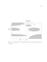
pressure of the vehicle and are a function of the vehicles’ shape and of the square of its
velocity. The center of pressure is also strongly dependent on vehicle’s shape. For a more in-
depth analysis of this subject see, for instance, (Hoerner, 1992).
With the exception of the gravity and buoyancy forces, these effects are best described in the
Body-Fixed Frame. Therefore, the remaining equations of motion, describing the vehicle’s
kinetics, can be presented in the following compact form:

act
)(g)(D)(CM
τ
=
η
+
ν
ν
+
ν
ν
+
ν
&
(11)
M is the constant inertia and added mass matrix of the vehicle, C(
ν) is the Coriolis and
centripetal matrix, D(
ν) is the Damping matrix, g(η) is the vector of restoring forces and
moments and
τ

act
is the vector of body-fixed forces from the actuators. We follow the
common formulation where the lift and drag terms are both accounted in the damping
matrix.
For vehicles with a streamlined shape, theoretical and empirical formulas may be used.
However, it must be remarked that in practice these vehicles are not quite as regular as
assumed in the formulas usually employed for added mass, drag and lift: they have
antennas, transducers and other protuberances that affect those effects, with special
incidence on the drag terms. Therefore we should look at the formulas as giving
underestimates of the true values of the coefficients.
In certain situations it may be useful to consider the following simplifications: if the
vehicle’s weight equals its buoyancy and the center of gravity is coincident with the center
of buoyancy,
g(η) is null; for an AUV with port/starboard, top/bottom and fore/aft
symmetries, M
and D(ν)=D
1
(ν)+D
2
(ν) are diagonal. In the later case, the damping matrix has
the following form:
)M,M,K,Z,Y,X(diag)(D
qqpwvu1
=
ν
(12)
|)r|N|,q|M|,p|K|,w|Z|,v|Y|,u|X(diag)(D
|r|r|q|q|p|p|w|w|v|v|u|u
2
=

ν
(13)
For low velocities, the quadratic terms on Eq. 13, such as Y
v|v|
|v|, may be considered
negligible. However, in practice, the fore/aft symmetry is rarely verified and non-diagonal
terms should be considered. Even so, certain simplifications can be further considered. For
instance, in torpedo shaped vehicles, some of the coefficients affecting the motion on the
vertical plane are the same as those affecting the motion on the horizontal plane, reducing
the number of different coefficients that must be estimated.
Some of the models found in the literature, e.g. (Prestero 2001; Leonard & Graver, 2001;
Conte & Serrani, 1996; Ridley et al., 2003), do not consider the linear damping terms
contained on D
1
(ν). These terms may play an important role in the design of the control
system, namely on local stability analysis. For low velocities scenarios the quadratic
damping terms become very small. If the linear damping is ignored, the linearization of the
system model around the equilibrium point may falsely reveal a locally unstable system.
This leads the control system designer to counteract by adding linear damping in the form
of velocity feedback, which potentially could be unnecessary, leading to conservative
designs. In fact, it is possible to find examples in the literature where the authors perform a
worst case analysis, by totally disregarding the damping matrix (Leonard 1996; Chyba 2003).
New Approaches in Automation and Robotics

204
2.2 Actuators
In the last years there has been a trend in the research of biologically inspired actuators for
underwater vehicles, see for instance (Tangorra, 2007). The development of vehicles
employing variable buoyancy and center of mass (e.g., gliders) is also underway
(Bachmayer, 2004). However, the preferred types of actuators for small size AUVs still are

electrically driven propellers and fins, due to its simplicity, robustness and low cost.
When high manoeuvrability is desired, full actuation is employed (for instance, with two
longitudinal thrusters, two lateral thrusters and two vertical thrusters). For over-actuated
vehicles, thruster allocation schemes may be applied in order to optimize performance and
power consumption. However, for a broad range of applications the cost effectiveness of
under-actuated vehicles is still a factor of preference. In those cases, a smaller number of
thrusters, eventually coupled with fins, is employed. This approach is applied in most
torpedo-like AUVs: there is a propeller for actuation in the longitudinal direction and fins
for lateral and vertical actuation. In this case,
τ
act
depends only on 3 parameters: propeller
velocity, horizontal fin inclination and vertical fin inclination.
Dynamic models for propellers can be found in (Fossen, 1994) and this is still an active area
of research (D'Epagnier, 2006). However, the dynamics of the thruster motor and fin servos
are generally faster than the remaining dynamics. Therefore, they can be frequently
excluded from the model, namely when operation at steady speed is considered as opposed
to dynamic positioning, or station keeping.
2.3 Simplified models
For a large class of underwater vehicles it is usual to consider decoupled modes of
operation, see for instance (Healey & Lienard, 1993), the most common being motion on the
horizontal plane, involving changes on x, y,
ψ, v, and motion on the vertical plane aligned
with the body fixed x-z axes, involving changes on z,
θ, w and q. In the later mode,
assuming small deviations from 0 on the pitch angle, a linearized model can be used
without introducing significant error (the a
ij
, k
w

and k
q
coefficients can be calculated as a
function of the coefficients of the full nonlinear model):
⎥
⎥
⎥
⎥
⎥
⎦
⎤
⎢
⎢
⎢
⎢
⎢
⎣
⎡
τ
τ
+
⎥
⎥
⎥
⎥
⎥
⎦
⎤
⎢
⎢

⎢
⎢
⎢
⎣
⎡
θ
⎥
⎥
⎥
⎥
⎥
⎦
⎤
⎢
⎢
⎢
⎢
⎢
⎣
⎡
−
=
⎥
⎥
⎥
⎥
⎥
⎦
⎤
⎢

⎢
⎢
⎢
⎢
⎣
⎡
θ
qq
ww
cz
444342
343332
k
k
0
v
q
w
z
aaa0
aaa0
1000
01u0
q
w
z
&
&
&
&

(14)
For the purpose path planning on the horizontal plane with piecewise continuous velocity, a
simple kinematic model can be used:
⎪
⎩
⎪
⎨
⎧
=ψ
+ψ+ψ=
+ψ−ψ=
r
v)sin(u)cos(vy
v)sin(v)cos(ux
cx
cx
&
&
&

(15)
For the purpose of path planning, it is considered that the actuators produce the desired
velocities instantaneously. The allowable ranges for u, v and r must be the same as the ones
Models for Simulation and Control of Underwater Vehicles

205
verified for the full dynamic model, or measured in real operation. While this model
introduces some errors that must be compensated later by the on-line control system, this is
very useful for the general path planning algorithms. If the vehicle does not possess lateral

actuation, such as a torpedo, the model drops the terms on v and becomes the well-known
unicycle model.
3. Results and discussion
In (Silva et al., 2007) we describe a simulation environment which allows us to simulate
AUV operation in real-time and with direct interaction with the control software. All
software was written in C++ and is based on the Dune framework, also developed at the
University of Porto. Using this framework, the control software and simulation engine may
run either on a desktop computer or on the final target computer. Our results show that
realistic real-time and faster than real-time simulation of underwater vehicles is quite
feasible in today’s computers. The trajectories obtained with the exact same inputs as those
used in experiments in the water differ slightly from the real trajectories. However, in what
concerns simulation of closed-loop operation, the feedback employed on the control laws
smoothes out the effects of parameter uncertainty. Therefore it is possible to observe a good
correlation between the performance of the controlled system in simulation and that
obtained in real operation. This conclusion is drawn using the exact same controllers and
timings on simulation and real operation. This result is not as assuring as a complete
analytical proof but, then again, none of the currently employed models are perfect
descriptions of the reality therefore, even an analytical study does not guarantee the
planned behaviour when the respective implementation comes to real life operation.
The available methods are quite satisfactory for high level mission planning and already
provide a good basis for initial controller tuning. However, additional tuning is still
required when it comes to real life vehicle operation. Research on models whose simulation
can be done in reasonable time while providing an increasing level of adherence to reality
should continue.
4. References
Bachmayer, R.; Leonard, N.E.; Graver, J.; Fiorelli, E.; Bhatta, P. & Paley, D. (2004).
Underwater gliders: recent developments and future applications,
Proceedings of the
2004 International Symposium on Underwater Technology
, pp. 195-200, Taipei, Taiwan,

April 2004
Brennen, C.E (1982).
A review of added mass and fluid internal forces, Naval Civil engineering
laboratory, California
Chyba, M.; Leonard, N. E. & Sontag, E. (2003). Singular trajectories in multi-input time-
optimal problems: Application to controlled mechanical systems,
Journal of
Dynamical and Control Systems, Vol. 9, No. 1, pp. 73-88
Conte, G. & Serrani, A. (1996) Modelling and simulation of underwater vehicles,
Proceedings
of the 1996 IEEE International Symposium on Computer-Aided Control System Design,
pp. 62-67, Dearborn, Michigan, September 1996
D'Epagnier, K. P. (2006). AUV Propellers: Optimal Design and Improving Existing
Propellers for Greater Efficiency,
Proceedings of the OCEANS 2006 MTS/IEEE
Conference
, Boston, Massachusetts USA, September 2006
New Approaches in Automation and Robotics

206
Fossen, T.I. (1994). Guidance and Control of Ocean Vehicles, John Wiley and Sons, Inc., New
York
Gertler, M. & Hagen, G. R. (1967).
Standard equations of motion for submarine simulation, Naval
Ship Research and Development Center, Report 2510.
Healey, A. J. & Lienard, D. (1993). Multivariable Sliding Mode Control for Autonomous
Diving and Steering of Unmanned Underwater Vehicles,
IEEE Journal of Oceanic
Engineering,
Vol. 18, No. 3, pp. 1-13

Leonard, N. E. (1996). Stabilization of steady motions of an underwater vehicle,
Proceedings
of the 1996 IEEE Conference on Decision and Control
, pp. 961-966, Kobe, Japan,
December 1996
Leonard, N. E. & Graver, J. G. (2001). Model-based feedback control of autonomous
underwater gliders,
IEEE Journal of Oceanic Engineering (Special Issue on Autonomous
Ocean-Sampling Networks)
, Vol. 26, No. 4, pp. 633-645
Lewis, E. (Ed.) (1989).
Principles of Naval Architecture (2nd revision), Society of Naval
Architects and Marine Engineers, Jersey City, New Jersey
Hoerner, S. F. & Borst H. V. (1992).
Fluid Dynamic Lift (second edition), published by author,
ISBN 9998831636
Irwin, R. P. & Chauvet, C. (2007). Quantifying Hydrodynamic Coefficients of Complex
Structures,
Proceedings of the IEEE/OES OCEANS 2007 - Europe, pp. 1-5, Aberdeen,
Scotland, June 2007
Nahon, M. (2006). A Simplified Dynamics Model for Autonomous Underwater Vehicles,
Journal of Ocean Technology, Vol. 1, No. 1, pp. 57-68
Prestero, T. J. (2001). Development of a six-degree of freedom simulation model for the
remus autonomous underwater vehicle,
Proceedings of the OCEANS 2001 MTS/IEEE
Conference and Exhibition, pp. 450-455, Honolulu, Hawaii, November 2001
Ridley, P.; Fontan, J. & Corke, P. (2003). Submarine dynamic modelling,
Proceedings of the
Australian Conference on Robotics and Automation, Brisbane, Australia, December
2003

Silva, J.; Terra, B.; Martins R. & Sousa, J. (2007). Modeling and Simulation of the LAUV
Autonomous Underwater Vehicle,
Proceedings of the 13th IEEE IFAC International
Conference on Methods and Models in Automation and Robotics
, pp. 713-718, Szczecin,
Poland, August 2007
Tangorra, J. L.; Davidson, S. N.; Hunter, I. W.; Madden, P. G. A.; Lauder, G. V.; Dong, H.;
Bozkurttas, M. & Mittal, R. (2007). The Development of a Biologically Inspired
Propulsor for Unmanned Underwater Vehicles,
IEEE Journal of Oceanic Engineering,
Vol. 32, No. 3, pp. 533-550
von Ellenrieder, K. D. & Ackermann, L. E. J. (2006). Force/flow measurements on a low-
speed, vectored-thruster propelled UUV,"
Proceedings of the OCEANS 2006
MTS/IEEE Conference, Boston, Massachusetts USA, September 2006
12
Fuzzy Stabilization of Fuzzy Control Systems
Mohamed M. Elkhatib and John J. Soraghan
University of Strathclyde
United Kingdom
1. Introduction
Recently there has been significant growth in the use of fuzzy logic in industrial and
consumer products (J. Yen 1995). However, although fuzzy control has been successfully
applied to many industrial plants that are mostly nonlinear systems, many critics of fuzzy
logic claim that there is no such thing as a stability proof for fuzzy logic systems in closed-
loop control (Reznik 1997; Farinwata, Filev et al. 2000). Since fuzzy logic controllers are
classified as "non-linear multivariable controllers" (Reznik 1997; Farinwata, Filev et al.
2000), it can be argued that all stability analysis methods applicable to these controller types
are applicable to fuzzy logic controllers. Unfortunately, due to the complex non-linearities of
most fuzzy logic systems, an analytical solution is not possible. Furthermore, it is important

to realize that real, practical problems have uncertain plants that inevitably cannot be
modelled dynamically resulting in substantial uncertainties. In addition the sensors noise
and input signal level constraints affect system stability. Therefore a theory that is able to
deal with these issues would be useful for practical designs. The most well-known time
domain stability analysis methods include Lyapunov’s direct method (Wu & Ch. 2000;
Gruyitch, Richard et al. 2004; Rubio & Yu 2007) which is based on linearization and
Lyapunov’s indirect method (Tanaka & Sugeno 1992; Giron-Sierra & Ortega 2002; Lin,
Wang et al. 2007; Mannani & Talebi 2007) that uses a Lyapunov function which serves as a
generalized energy function. In addition many other methods have been used for testing
fuzzy systems stability such as Popov’s stability criterion (Katoh, Yamashita et al. 1995;
Wang & Lin 1998), the describing function method (Ying 1999; Aracil & Gordillo 2004),
methods of stability indices and systems robustness (Fuh & Tung 1997; Espada & Barreiro
1999; Zuo & Wang 2007), methods based on theory of input/output stability (Kandel, LUO
et al. 1999), conicity criterion (Cuesta & Ollero 2004). Also there are methods based on
hyper-stability theory (Piegat 1997) and linguistic stability analysis approach (Gang & Laijiu
1996).
Fuzzy logic uses approximate reasoning and in this chapter a practical algorithm to improve
system stability by using a fuzzy stabilizer block in the feedback path is introduced. The
fuzzy stabilizer is tuned such that its nonlinearity lies in a bounded sector resulting from the
circle criterion theory (Safonov 1980). The circle criterion presents the sufficient condition
for absolute stability (Vidyasagar 1993). An appealing aspect of the circle criterion is its
geometric nature, which is reminiscent of the Nyquist criterion. It is a frequency domain
method for stability analysis and has been used by Ray et al (1984) to ensure fuzzy system
stability (Ray, Ghosh et al. 1984; Ray & Majumderr 1984).
New Approaches in Automation and Robotics

208
Throughout this chapter we use a practical approach to stabilize fuzzy systems with the aid
of the circle criterion theory using a Takagi-Sugeno fuzzy block in the feedback loop of the
closed system. The new technique is used to ensure stability for the proposed robot fuzzy

controller. Furthermore, the study indicates that the fuzzy stabilizer can be integrated, with
minor modifications, into any fuzzy controller to enhance its stability. As a result, the
proposed design is suitable for hardware implementation even permitting relatively simple
modification of existing designs to improve system stability. In addition an extension to the
approach to stabilize MIMO (Multi-input Multi-output) systems is also presented.
2. Problem formulation and analysis
This chapter concentrates on the stability of a closed loop nonlinear system using a Takagi-
Sugeno (T-S) fuzzy controller. Fuzzy control based on Takagi-Sugeno (T-S) fuzzy model
(Babuska, Roubos et al. 1998; Buckley & Eslami 2002) has been used widely in nonlinear
systems because it efficiently represents a nonlinear system by a set of linear subsystems.
The main feature of the T-S fuzzy model is that the consequents of the fuzzy rules are
expressed as analytic functions. The choice of the function depends on its practical
applications. Specifically, the T–S fuzzy model is an interpolation method, which can be
utilized to describe a complex or nonlinear system that cannot be exactly modelled
mathematically. The physical complex system is assumed to exhibit explicit linear or
nonlinear dynamics around some operating points. These local models are smoothly
aggregated via fuzzy inferences, which lead to the construction of complete system
dynamics.
Takagi-Sugeno (T-S) fuzzy controller is used in the feedback path as shown in Fig.1, so that
it can change the amount of feedback in order to enhance the system performance and its
stability.


Fig. 1 The proposed System block diagram
The proposed fuzzy controller is a two-input one-output system: the error e(t) and the
output y(t) are the controller inputs while the output is the feedback signal ϕ(t). The fuzzy
controller uses symmetric, normal and uniformly distributed membership functions for the
rule premises as shown in Fig.2(a) and 2(b). Labels have been assigned to every membership
function such as NBig (Negative Big) and PBig (Positive Big) etc. Notice that the widths of
the membership functions of the input are parameterized by L and h which are used to tune

the controller and limited by the physical limitations of the controlled system.
Fuzzy Stabilization of Fuzzy Control Systems

209

Fig. 2 (a) The membership distribution of the 2nd input, open loop output y(t)


Fig. 2 (b) The membership distribution of the 1st input, the error e(t)
While using the T-S fuzzy model (Buckley & Eslami 2002), the consequents of the fuzzy
rules are expressed as analytic functions which are linearly dependent on the inputs. In
present case, three singleton fuzzy terms are assigned to the output such that the consequent
part of the i
th
rule ϕ
c
i
is a linear function of one input y(t) which can be expressed as:
)()( tyMrt
i
c
i
=
ϕ
(1)
where r
i
takes the values -1, 0, 1
(depends on the output’s fuzzy terms)
y(t) is the 2nd input to the controller

M is a parameter used to tune the controller.
The fuzzy rules are formulated such that the output is a feedback signal inversely
proportional to the error signal as follow:
IF the error is High THEN
)(
1
tyM
c
=
ϕ

IF the error is Normal THEN
0
2
=
c
ϕ

IF the error is Low THEN
)(
3
tyM
c
−=
ϕ

The fuzzy controller is adjusted by changing the values of L, h and M which affect the
controller nonlinearity map. Therefore, the fuzzy controller implements these values
New Approaches in Automation and Robotics

210
equivalent to the saturation parameters of standard saturation nonlinearity (Jenkins &
Passino 1999).
Before studying the system stability, a general model of a Sugeno fuzzy controller is defined
(Thathachar & Viswanath 1997; Babuska, Roubos et al. 1998; Buckley & Eslami 2002) as
follows:
For a two-input T-S fuzzy system; let the system state vector at time t be:
⎥
⎦
⎤
⎢
⎣
⎡
=
2
1
z
z
z
where z
1
, and z
2
are the state variable of the system at time t.
A T-S fuzzy system is defined by the implications such that:
nn
ii
i
BzAz
thenSiszANDSiszifR

+=
&
)(:
2211

and for the proposed system where B
n
is taken as a zero matrix and n = 2 for the two-input
system, then:
2211
2211
)(:
zAzAz
thenSiszANDSiszifR
ii
i
+=
&

for i = 1 … N,
where S
i
1
, S
i
2
are the fuzzy set corresponding to the state variables z
1
, z
2

and R
i
.
A
n
=[A
1
, A
2
], are the characteristic matrices which represent the fuzzy system.
However the truth value or weight of the implication R
i
at time t denoted by w
i
(z) is defined
as:
))(),((∧)(
21
21
zzzw
ii
SS
i
μ
μ
=

where
µ
S

(z) is the membership function value of fuzzy set S at position z
^ is taken to be the min operator
Then the system state is updated according to (Reznik 1997):

∑
∑
∑
=
=
=
==
N
i
ii
N
i
i
N
i
ii
zAz
zw
zAzw
z
1
1
1
)(
)(
)(

δ
&
(2)
where
∑
=
=
N
p
p
i
i
zw
zw
z
1
)(
)(
)(
δ

However, the consequent part of the proposed system rules is a linear function of only one
input y(t) as mentioned in the pervious section, and therefore the output of the fuzzy
controller is of the form:
Fuzzy Stabilization of Fuzzy Control Systems

211

∑
=

=
N
i
ii
yMyy
1
)(
δ
&
(3)
where N is the number of the rules
M
i
is a parameter used for the i
th
rule to tune the controller
Notice that Eq. 3 directly depends on the input y(t) and indirectly depends on e(t) which
affects the weights δ
i
. Thus the proposed system can be redrawn as shown in Fig. 3


Fig. 3 The equivalent block diagram of the proposed system
The stability analysis of the system considers the system nonlinearities and uses circle
criterion theory to ensure stability.
3. Stability analysis using circle criterion
In this section the circle criterion (Ray, Ghosh et al. 1984; Ray & Majumderr 1984;
Vidyasagar 1993; Jenkins & Passino 1999) will be used for testing and tuning the controller
in order to ensure the system stability and improve its output response. The circle criterion
was first used in (Ray, Ghosh et al. 1984; Ray & Majumderr 1984) for stability analysis of

fuzzy logic controllers and as a result of its graphical nature; the designer is given a physical
feel for the system.
The output of the system given by Eq. 3 can be rewritten as follow:

()
[]
{}
∑
=
−−=
N
i
iii
yMyyMy
1
)(1
δ
&
(4)
This comprises a separate linear part and nonlinear part denoted as ϕ(t) that can be
expressed by (Vidyasagar 1993; Cuesta, Gordillo et al. 1999):

()
[]
∑
=
−=
N
i
ii

yMy
1
)(1
δϕ
(5)
As a result a T-S fuzzy system can be represented according to a LUR’E system (Vidyasagar
1993; Cuesta, Gordillo et al. 1999). Consider a closed loop system, Fig. 4, given a linear time-
invariant part G (a linear representation of the process to be controlled) with a nonlinear
feedback part ϕ(t) (represent a fuzzy controller).
The function ϕ(t) represents memoryless, time varying nonlinearity with:
ℜ
→
ℜ
×
∞
),0[:
ϕ

New Approaches in Automation and Robotics

212

Fig. 4 T-S Fuzzy System according to the structure of the problem of LUR’E
If ϕ is bounded within a certain region as shown in Fig. 5 such that there exist:
α, β, a, b, (β>α, a<0<b) for which:

yyy
β
ϕ
α

≤
≤
)( (6)


Fig. 5 Sector Bounded Nonlinearity
for all t ≥ 0 and all y ∈ [a, b] then: ϕ(y) is a “Sector Nonlinearity”:
Fuzzy Stabilization of Fuzzy Control Systems

213
If
yyy
β
ϕ
α
≤≤ )( is true for all y ∈ (-∞,∞) then the sector condition holds globally and the
system is “absolutely stable”. The idea is that no detailed information about nonlinearity is
assumed, all that known it is that ϕ satisfies this condition (Vidyasagar 1993).
Let D(α, β) denote the closed disk in the complex plane centred at -
αβ
βα
2
)( +
, with radius
αβ
βα
2
−
and the diameter is the line segment connecting the points
0

1
j+
−
α
and 0
1
j+
−
β
.
The circle criterion states that when ϕ satisfies the sector condition Eq.6 the system in Fig.3
is absolutely stable if one of following conditions are met (Vidyasagar 1993):
• If 0 < α < β, the Nyquist Plot of G(jw) is bounded away from the disk D(α, β) and
encircles it m times in the counter clockwise direction where m is the number of poles
of G(s) in the open right half plane(RHP).
• If 0 = α < β, G(s) is Hurwitz (poles in the open LHP) and the Nyquist Plot of G(jw) lies
to the right of the line
β
1−
=
s .
• If α < 0 < β, G(s) is Hurwitz and Nyquist Plot of G(jw) lies in the interior of the disk
D(α, β) and is bounded away from the circumference of D(α, β).
For the fuzzy controller represented by Eq. 2, we are interested in the first two conditions
(Ray & Majumderr 1984), and it can be sector bounded in the same manner (Jenkins &
Passino 1999) as described next.
Consider the fuzzy controller as a nonlinearity
ϕ and assume that there exist a sector (α, β)
in which
ϕ lies, then use the circle criterion to test the stability. Simply, using the Nyquist

plot, the sector bounded nonlinearity of the fuzzy logic controller will degenerate,
depending on its slope α that is always zero (Jenkins & Passino 1999) and the disk to the
straight line passing through
β
1−
and parallel to the imaginary axis as shown in Fig.6 In
such case the stability criteria will be modified as follows (Vidyasagar 1993):
Definition: A single-input single-output (SISO) system will be globally and asymptotically
stable provided the complete Nyquist locus of its transfer function does not enter the
forbidden region left to the line passing through
β
1−
in an anticlockwise direction as shown
in Fig. 6.
The fuzzy controller is tuned until its parameters lie in the bounded sector, so that the fuzzy
system nonlinearity is bounded in this sector. In fact, even if the function
ϕ is approximately
linear, the saturation outside this region causes
ϕ to be always nonlinear.
From the above discussion, we conclude that to ensure stability for a closed loop system
with known transfer function or nonlinearity sector, one can add a fuzzy block (stabilizer) in
the feedback loop tuned in the manner described above and under the condition that the
stabilizer block is faster than the controlled system. This concept is used to enhance the
performance of existing control systems especially for systems controlled using fuzzy
controller in the forward loop. In such cases the feedback fuzzy stabilizer can be integrated
in the main fuzzy controller as explained in the next section.
New Approaches in Automation and Robotics

214

Fig. 6 Nyquist plot with fuzzy feedback system (Ray & Majumderr 1984).
4. Self stabilized fuzzy controller
Figure 7 comprises a plant controlled by a SISO fuzzy controller. In order to guarantee the
system stability, a fuzzy stabilizer has been added in the feedback path.


Fig. 7 Block Diagram of the system with Fuzzy-P controller
Only, minor changes are necessary to the above analysis in order to include the SISO fuzzy
controller nonlinearities if these have not been included in the previously calculated sector.
As a result, the fuzzy stabilizer will be retuned to the new sector which will be the minimum
intersection between the fuzzy controller nonlinearity sector and the sector results using the
circle criterion. This is understandable as the fuzzy controller represents an odd function
(Reznik 1997; Jenkins & Passino 1999) (i.e.
ϕ(-y) = - ϕ(y)) , so that fuzzy controller can be in
the feedback path rather than the feed forward path. Therefore, the dominant nonlinear
sector will be the minimum sector. Consequently from analysis, the feedback stabilizer can
be built in each fuzzy controller to improve its performance by adding an extra input and
modifying the original fuzzy rule base by adding the stabilization rules.
Generally, there are many types of fuzzy reasoning that can be employed in fuzzy control
applications, the most commonly used types are Mamdani and Takagi-Sugeno (T-S) type.
For Mamdani fuzzy systems (Farinwata, Filev et al. 2000), the same structure can be used
Fuzzy Stabilization of Fuzzy Control Systems

215
except for the addition of another input y(t) and three extra rules to the rule base as shown
in Fig. 8.


Fig. 8 The modification to the fuzzy system structure
Where µ

x
, µ
c
are the input and output fuzzy sets for Mamdani fuzzy system
µ
y
, µ
A
are the input and output fuzzy sets for fuzzy stabilizer system
Consequently, less modification is required for T-S type fuzzy systems.
The main reason for integrating the stabilizer into the normal structure of fuzzy controllers
is to make them suitable for hardware and software implementation. The same design of the
circuits or algorithms will be used without significant modifications.
5. Examples and simulation results
A plant with transfer function:
4084.10
400
)(
23
+++
=
sss
sG
,
is used to demonstrate the performance of fuzzy stabilizer. The Nyquist plot of G(jw) is
shown in Fig. 9.
The system is unstable and has closed loop poles at -12.6 and 1.08± j 5.82, with a gain margin
of -19.3dB. If we consider the fuzzy stabilizer as a nonlinearity
ϕ as shown in Fig. 5, then the
disk D(α, β) is the line segment connecting the points

0
1
j+
−
α
and
0
1
j+
−
β
. Applying the
Circle Criterion and because α = 0 the second condition will be used. To find a sector (α, β)
New Approaches in Automation and Robotics

216
in which
ϕ lies, the system Nyquist plot Fig. 9 is analyzed. The Nyquist plot does not satisfy
the second condition as it intersects with the line drawn at
259.9
1
−=
−
β
. In order to meet the
second condition of the theory the line drawn at
β
1−
will be moved to be at 5.27
1

−=
−
β
such
that the Nyquist plot lies to the right of it. As a result, the fuzzy controller will be tuned by
choosing M, and L such that its nonlinearities lies in the sector (0,0.036).



Fig. 9 The plant Nyquist plot
In order to satisfy the circle criterion condition, the ratio M/L will be kept less than β (i.e
M/L < 0.036) by choosing M = 0.68 and L = 20 .
A traditional fuzzy like proportional controller (Reznik 1997) is used to control the system
with a normal feedback loop as we saw in Fig. 7 in order that a comparison can be made
between the results with and without a fuzzy stabilizer in the feedback loop. In order to
retune the fuzzy stabilizer, the fuzzy P-controller has a ratio M
c
/L
c
or β
c
= 1.
However β = 0.036 for the plant, and therefore the minimum sector for the stabilizer to be
tuned is: (α, β) = (0, 0.036).
The system step response (solid line) results with and without the use of the stabilizer
(dashed line) are shown Fig. 10. The results shows that the system with the fuzzy
P-controller in Fig. 7 yields an unstable output (dashed line) while the use of the stabilizer
produces a stable output.
The approach described has provided a quick and easy stabilization process which can
allow designers to fine tune their controller’s performance without at the same time, being

worried about stability issues.
Fuzzy Stabilization of Fuzzy Control Systems

217
In Fig. 11 (a), and (b), the step responses for different systems, according to the setup in Fig.
3, are shown. The simulations show the tested system for a normal feedback without the
stabilizer and with adding the stabilizer in the feedback loop as in illustrated in Fig. 3.
Using the same algorithm given a transfer function, a nonlinearity sector and the tuned
values of M and L of the fuzzy stabilizer, the stabilizer has been tuned.


Fig. 10 The simulated step response of the two compared systems


Fig. 11(a) The step Response of the controller with following parameters (Black curve):
1577
12
)(
23
+++
=
sss
sG
, (α, β)=(0, 0.3), L=1, M= 0.3
with a stabilizer in the feedback loop
with normal feedback
New Approaches in Automation and Robotics

218

Fig. 11(b) The step Response of the controller with following parameters (Black curve):
34
40
)(
2
++
=
ss
sG
, (α, β) = (0, 1.3), L=1, M = 1.3
6. Extension to MIMO fuzzy systems
The stability analysis of multi-inputs multi-outputs (MIMO) is a nontrivial task due to the
complexity of the system (Safonov 1980), however, many algorithms have been proposed to
tackle the problem; K. Ray and D. Majumder (Ray & Majumderr 1984) extended their
approach of using circle criteria to MIMO systems but restricted the result to square systems
only. The conicity theory has been used by others (Kang, Kwon et al. 1998; Cuesta, Gordillo
et al. 1999; Cuesta & Ollero 2004) to study the stability of MIMO fuzzy systems but it suffers
from the nontrivial problem of determining the candidate centre. Linear matrix inequalities
(LMI) technique is also used (Wang, Tanaka et al. 1996; Lam & Seneviratne 2007) but has the
disadvantage of high number of LMI used which make the analysis more complicated
(Cuesta, Gordillo et al. 1999). The description function is also used to study the stability of
MIMO systems (Abdelnour, Cheung et al. 1993; Aracil & Gordillo 2004).
6.1 Stability analysis of open loop MIMO systems
In order to extend the proposed approach fuzzy stabilizer to MIMO (Multi-input Multi-
output) systems, an additively decomposition technique (Ying 1996) is used. According to
the structure of the classical problem of LUR’E (Vidyasagar 1993; Cuesta, Gordillo et al.
1999) shown in Fig. 4 , and referring to the analysis in section 3, a T-S fuzzy system can be
represented as linear and nonlinear part as follows:
Consider a T-S fuzzy system with N rules (Cuesta, Gordillo et al. 1999):
zMz

thenSiszANDSiszifR
ij
j
i
r
=
&
)(:
2
211

with a stabilizer in the feedback loop
with normal feedback
Fuzzy Stabilization of Fuzzy Control Systems

219
with:
⎥
⎥
⎦
⎤
⎢
⎢
⎣
⎡
=
ji
ji
ij
dc

ba
M
and
⎥
⎦
⎤
⎢
⎣
⎡
=
2
1
z
z
z

for r = 1 … m×n, where
S
i
1
, S
j
2
are the fuzzy membership function corresponding to the state variables
z
1
, z
2
, which represented by linguistic terms with membership functions such that:
0)0(,1)0(

11
11
=
=
=
=
zz
ip
SS
μ
μ

i ≠ p, i = 1, …, m
and
0)0(,1)0(
22
22
=
=
=
=
zz
jq
SS
μ
μ

j ≠ q, j = 1, …, n
and M
ij

∈ R
2x2
, is the characteristic matrices which represents the fuzzy system.
Similar to the analysis in section 2, the system state is updated according to:

∑∑
==
=
m
i
n
j
ijij
zMzz
11
)(
δ
&
(7)
where
∑∑
==
=
m
k
n
p
kp
ij
ij

zw
zw
z
11
)(
)(
)(
δ


and w
ij
(z) is the truth value or weight of the implication R
ij
at time t
Then Eq. 7 can be rewritten as:

()
[]
{}
∑∑
==
−−=
m
i
n
j
ijijij
zMzzMz
11

)(1
δ
&
(8)
Eq. 8 shows the system has been split into linear and nonlinear part, Fig. 4. Notice that the
first column of M
ij
depends on i while the second column depends on j Hence, the resulting
nonlinear part
ϕ(z) such that:

()
∑∑
==
−=
m
i
n
j
ijij
zMzz
11
)(1)(
δϕ
(9)
is additively decomposable (Cuesta, Gordillo et al. 1999), that is:

ϕ(z) = ϕ(z
1
, z

2
) = ϕ(z
1
, 0) + ϕ(0, z
2
) (10)
(see (Cuesta, Gordillo et al. 1999) for the proof)
New Approaches in Automation and Robotics

220
Eq. 10 implies that the nonlinear part ϕ is additively decomposable, and therefore
techniques used for stability analysis of SISO system can be used to stabilize the multi-input
multi-output systems. This can be done by adding a number of small fuzzy systems equal to
the number of the output variables in the feedback loop of the MIMO system for each input
variable as shown in Fig. 12. In this way all the nonlinearities of the fuzzy system can be
included within a bounded sector.


Fig. 12 The proposed MIMO fuzzy feedback system
6.2 Stability analysis of closed loop MIMO system
A simple stability analysis for closed loop system is shown in Fig. 13 (a). In this system the
proposed fuzzy stabiliser is placed on each feedback loop for each input as shown in Fig.
13(b). That includes all the nonlinearities of the system.


Fig. 13.(a) MIMO closed loop system
Fuzzy Stabilization of Fuzzy Control Systems

221

Fig. 13.(b) MIMO closed loop system with fuzzy stabilizers
6.3 Simulation example
Consider a MIMO system with a state space representation:
⎥
⎦
⎤
⎢
⎣
⎡
⎥
⎥
⎥
⎦
⎤
⎢
⎢
⎢
⎣
⎡
+
⎥
⎥
⎥
⎦
⎤
⎢
⎢
⎢
⎣
⎡

⎥
⎥
⎥
⎦
⎤
⎢
⎢
⎢
⎣
⎡
−−−
=
⎥
⎥
⎥
⎦
⎤
⎢
⎢
⎢
⎣
⎡
2
1
3
2
1
3
2
1

00
10
01
010
001
5077
u
u
x
x
x
x
x
x
&
&
&

⎥
⎥
⎥
⎦
⎤
⎢
⎢
⎢
⎣
⎡
⎥
⎦

⎤
⎢
⎣
⎡
−
=
⎥
⎦
⎤
⎢
⎣
⎡
3
2
1
2
1
010
001
x
x
x
y
y

In our problem we will find a transfer function of the model of the form:

⎥
⎦
⎤

⎢
⎣
⎡
⎥
⎦
⎤
⎢
⎣
⎡
=
⎥
⎦
⎤
⎢
⎣
⎡
2
1
2221
1211
2
1
u
u
GG
GG
y
y

where

5077
23
2
11
+++
=
sss
s
G


5077
23
21
+++
−
=
sss
s
G


5077
507
23
12
+++
+
=
sss

s
G


5077
7
23
2
22
+++
+
=
sss
ss
G

Using the analysis described in section 5 and by aid of Nyquist plot of the system as shown
in Fig. 14 we can determine
45.6
1
−=−
β
, as a result M/L ≤ 0.155.
Note that, for all the components of the system (G11, G12, G21, and G22), the denominator
in each case remains the same, since it holds the key to the system stability.
New Approaches in Automation and Robotics

222

Fig. 14 The Nyquist plot of the simulated system

The outputs of the open loop system show the system instability as shown in Fig. 15.


Fig. 15 The open loop response of the simulated system
Fuzzy Stabilization of Fuzzy Control Systems

223
When the fuzzy stabilizers are added to the system according to Fig. 12 and the fuzzy
parameters are set such that the ratio M/L ≤ 0.007 is kept the same as follow:
Stabilizer (1) M11= 3.1 , L11= 25
Stabilizer (2) M12= 1.8 , L12= 12
Stabilizer (3) M21= 0.031 , L21= 0.25
Stabilizer (4) M22= 0.018 , L22= 0.12
The simulation results in Fig. 16 show the output of the stabilized system.


Fig. 16 The outputs of the stabilized simulated system
The proposed technique has the advantage of keeping the system stable even if the system
nonlinearities have been changed provided that they still remain within the bounded sector
proposed.
7. Conclusion
This chapter presented a practical approach to stabilize fuzzy systems based on adaptive
nonlinear feedback using a fuzzy stabilizer in the feedback loop. For this we needed to
identify the nonlinearity range of the system. The fuzzy stabilizer is tuned so that the system
nonlinearities lie in a bounded sector as delivered by using the circle criterion theory.
Because of circle criterion’s graphical nature; the designer is given a physical feel for the
system. The concept has been used to ensure stability of a car-like robot controller. In
addition, the idea has been extended to stabilize MIMO systems based on the additively
decomposition technique.
New Approaches in Automation and Robotics

224
The advantage of the proposed approach is the simplicity of the design procedure especially
for the MIMO systems analysis and implementation. The use of the fuzzy system to control
the feedback loop using its approximate reasoning algorithm gives a good opportunity to
handle the practical system uncertainty. The approach described have provided a quick and
easy stabilization process which can allow designers to fine tune their controllers
performance without at the same time, worrying about stability issues It is also shown that
the fuzzy stabilizer can be integrated, with small modifications, in any fuzzy controller to
enhance its stability. As a result it is suitable for hardware implementation or even to
modify existence software and hardware design if required to ensure system stability.
8. References
Abdelnour, G., J. Y. Cheung, et al. (1993). "Application of Describing Functions in the
Transient Respose Analysis of Three Term Fuzzy Controller." IEEE Transaction on
System, Man and Cybernetics 23: 603-606.
Aracil, J. and F. Gordillo (2004). "Describing function method for stability analysis of PD and
PI fuzzy controllers." Fuzzy Sets and Systems 143: 233-249.
Babuska, R., J. Roubos, et al. (1998). Identification of MIMO systems by input-output TS
fuzzy models. In the proceedings of The 1998 IEEE International Conference on
Fuzzy systems, IEEE World Congress on Computational Intelligence.
Buckley, J. J. and E. Eslami (2002). An Introduction to Fuzzy Logic and Fuzzy Sets, Phydica-
Verlag Heidelberg.
Cuesta, F., F. Gordillo, et al. (1999). "Stability Analysis of Nonlinear Multivariable Takagi–
Sugeno Fuzzy Control Systems." IEEE Transaction on Fuzzy Systems 7(5): 508-520.
Cuesta, F. and A. Ollero (2004). "Fuzzy control of reactive navigation with stability analysis
based on conicity and Lyapunov theory." Journal of Control Engineering Practice
12: 625-638.
Espada, A. and A. Barreiro (1999). "Robust stability of fuzzy control systems based on
conicity conditions." Automatica 35: 643-654.
Farinwata, S. S., D. Filev, et al. (2000). Fuzzy Control: Synthesis and Analysis, John Wiley &

Sons Ltd.
Fuh, C C. and P C. Tung (1997). "Robust stability analysis of fuzzy control systems." Fuzzy
Sets and Systems 88: 289-298.
Gang, J. and C. Laijiu (1996). "Linguistic stability analysis of fuzzy closed loop control
systems." Fuzzy Sets and Systems 82: 27-34.
Giron-Sierra, J. M. and G. Ortega (2002). A Survey of Stability of Fuzzy Logic Control with
Aerospace Applications. 15th Triennial World Congress. Barcelona, Spain.
Gruyitch, L., J P. Richard, et al. (2004). Stability Domains, Chapman& Hall/CRC.
J. Yen, R. L., and L. A. Zadeh (1995). Industrial applications of fuzzy logic and intelligent
systems, IEEE Press.
Jenkins, D. and K. M. Passino (1999). "An Introduction to Nonlinear Analysis of Fuzzy
Control Systems." Journal of Intelligent and Fuzzy Systems, 17(1): 75–103.
Kandel, A., Y. LUO, et al. (1999). "Stability analysis of fuzzy control systems." Fuzzy Sets
and Systems 105: 33-48.
Fuzzy Stabilization of Fuzzy Control Systems

225
Kang, H J., C. Kwon, et al. (1998). "Robust Stability Analysis and Design Method for the
Fuzzy Feedback Linearization Regulator." IEEE Transaction on Fuzzy Systems 6(4):
464-472.
Katoh, R., T. Yamashita, et al. (1995). "Stability analysis of control system having PD type of
fuzzy controller." Fuzzy Sets and Systems 74: 321-334.
Lam, H. K. and L. D. Seneviratne (2007). "LMI-based stability design of fuzzy controller for
nonlinear systems." IET Control Theory Appl. 1(1): 393-401.
Lin, C., Q G. Wang, et al. (2007). "Stability conditions for time-delay fuzzy systems using
fuzzy weighting-dependent approach." IET Control Theory Appl. 1(1): 127-132.
Mannani, A. and H. A. Talebi (2007). "A Fuzzy Lyapunov-Based Control Strategy for a
Macro–Micro Manipulator: Experimental Results." IEEE Transactions on Control
Systems Technology 15(2): 375-383.
Piegat, A. (1997). Hyperstability of fuzzy-control systems and degrees of freedom. In the

proceedings of EUFIT’97.
Ray, K. S., A. M. Ghosh, et al. (1984). "L2-Stability and the related design concept for SISO
linear systems associated with fuzzy logic controllers." IEEE Transactions on
Systems, Man, and Cybernetics SMC-14(6): 932–939.
Ray, K. S. and D. D. Majumderr (1984). "Application of circle criteria for stability analysis of
linear SISO and MIMO systems associated with fuzzy logic controllers." IEEE
Transactions on Systems, Man, and Cybernetics SMC-14(2): 345–349.
Reznik, L. (1997). Fuzzy Contollers, Newnes.
Rubio, J. d. J. and W. Yu (2007). "Stability Analysis of Nonlinear System Identification via
Delayed Neural Networks." IEEE TRANSACTIONS ON CIRCUITS AND
SYSTEMS-II: EXPRESS BRIEFS 54(2): 161-165.
Safonov, M. G. (1980). Stability and Roboustness of Multivariable Feedback Systems. Unites
State of America, The Massachusetts Institute Of Technology.
Safonov, M. G. (1980). Stability and Robustness of Multivariable Feedback systems, The
Massachusetts Institute of Technology.
Tanaka, K. and M. Sugeno (1992). "Stability analysis and design of fuzzy control systems."
Fuzzy Sets and Systems 45: 135-156.
Thathachar, M. A. L. and P. Viswanath (1997). "On the stability of fuzzy systems." IEEE
Transaction on Fuzzy Systems 5(1): 145-151.
Vidyasagar, M. (1993). Nonlinear Systems Analysis. Englewood, Cliffs, New Jersey, Prentice
Hall, Inc.
Wang, H. O., K. Tanaka, et al. (1996). "An Aproach to Fuzzy Control of Nonlinear Systems:
Stability and Design Issues." IEEE Trans. Fuzzy Systems 4: 14-23.
Wang, W. J. and H. R. Lin (1998). "Fuzzy control design for the trajectory tracking in phase
plane." IEEE Transaction on System, Man and Cybernetics, part A 28(5): 710-719.
Wu, S. J. and T. L. Ch. (2000). "Optimal fuzzy controller design: Local concept approach."
IEEE Trans. Fuzzy Systems 8(2): 171-185.
Ying, H. (1996). "Structure Decomposition of the General MIMO Fuzzy Systems."
International Journal of Intelligent Control and Systems 1(3): 327-337.
New Approaches in Automation and Robotics

226
Ying, H. (1999). "Analytical analysis and feedback linearization tracking control of the
general Takagi-Sugeno fuzzy dynamic systems." IEEE Transaction on system, Man
and Cybernetics, part C 29(2): 290-298.
Zuo, Z. and Y. Wang (2007). "Robust stability and stabilisation for nonlinear uncertain time-
delay systems via fuzzy control approach." IET Control Theory Appl. 1(1): 422-429.


13
Switching Control in the Presence of
Constraints and Unmodeled Dynamics
Vojislav Filipovic
Regional center for talents, Loznica
Serbia

1. Introduction
Recently there has been increased research interest in the study of the hybrid dynamical
systems (Sun & Ge, 2005) and (Li et al., 2005). These systems involve the interaction of
discrete and continuous dynamics. Continuous variables take the values from the set of real
numbers and the discrete variables take the values from finite set of symbols. The hybrid
systems have the behaviour of an analog dynamic system before certain abrupt structural or
operating conditions are changed. The event driven dynamics in hybrid control systems can
be described using different frameworks from discrete event systems (Cassandras &
Lafortune, 2008) such as timed automata, max-plus algebra or Petry nets. For dynamic
systems whose component are dominantly discrete event, main tools for analysis and design
are representation theory, supervisory control, computer simulation and verification. From
the clasical control theory point of view, hybrid systems may be considered as a switching
control between analog feedback loops. Generally, hybrid systems can achieve better
performance then non-switching controllers because they can to reconfigure and reorganize

their structures. For that is necessery correct coordination of discrete and analog control
variables.
The mathematical model for real process, generally, has the Hammerstein-Wiener form
(Crama & Atkins, 2001) and (Zhao & Chen, 2006). It means that on the input and output of
the process are present nonlinear elements (actuator and sensor). Here we will consider
Hammerstein model which has the input saturation as nonlinear element. That is the most
frequent nonlinearity encountered in practice (Hippe, 2006). Also, unmodeled dynamics
with matching condition is present. As a control strategy will be used switching control. The
switched systems can be viewed as higher abstraction of hybrid systems.
The design of switching controllers having guaranted stability, known as the picewise linear
LQ control (PLC), is first considered in (Wredenhagen & Belanger, 1994). The picewise
linear systems are systems that have different linear dynamics in different regions of the
continuous state space (Johansson, 2003). The PLC control has the associated switching
surfaces in form of positively invariant sets and yields a relatively low-gain controller. In the
LHG (low-and-high gain) design a low gain feedback law is first designed in such a way