Mechanics Analysis 2010 Part 5 ppt
Bạn đang xem bản rút gọn của tài liệu. Xem và tải ngay bản đầy đủ của tài liệu tại đây (966.35 KB, 35 trang )
126
Mechanics and analysis
of
composite materials
The name “complementary” becomes clear if we consider a bar in Fig.
1.1
and the
corresponding stress-strain curve in Fig.
4.8.
The area
OBC
below the curve
represents
U
in accordance with the first equation in
Eqs.
(4.8), while the area
OAB
above the curve is equal to
U,.
As
was shown in Section
2.9,
dU in Eqs. (4.8) is an
exact differential. To prove the same for dU,, consider the following sum:
which is obviously an exact differential. Since dU in this sum is also an exact
differential, dU, should have the same property and can be expressed as
Comparing this result with
Eq.
(4.9),
we arrive at Castigliano’s formulas
(4.10)
which are valid for any elastic solid (for a linear elastic solid,
U,
=
U).
Complementary potential,
U,,
in general, depends on stresses, but for an isotropic
material,
Eq.
(4.10)
should yield invariant constitutive equations that do not depend
on the direction of coordinate axes. This means that
U,
should depend on stress
invariants
11~12,
I3
in Eqs. (2.13). Assuming different approximations for function
Uc(Zl,
Z2,
I3)we can construct different classes of nonlinear elastic models. Existing
experimental verification of such models shows that dependence
U,
on
13
can be
neglected. Thus, we can present complementary potential in
a
simplified form
U,
(ZI,
Z2)and expand this function into the Taylor series as
E
C
E
de
Fig.
4.8.
Geometric interpretation
of
elastic potential. U. and complementary potential, U,.
Chapter
4.
Mechanics
of
a
composite
layer
127
1
1 1
2
3!
4!
u,
=
c0
+
c~~I~
+
-clzif
+
-cI31;
+-cI4if
+
+
C2li2
+
-c2&
+ ??I;
+
-c,4i;
+
1
1
I
2
3!
4!
+
-CI~ZIZII~
1
+-c1221iji2
1
3 1
+-~112211122
2
3!
3!
1 1
1
4! 4! 4!
+-cI3,1.l:i2 +-c12,21:i; +-c1123i1i;3
+
,
(4.1
1)
where
Constitutive equations follow from Eq. (4.10) and can be written in the form
au,
ai,
au,
aiz
E
‘I
-
ail
aoij
ai,
aoii
.
(4.12)
Assuming that for zero stresses
U,
=
0
and
cij
=
0 we should take co
=
0 and
CI
I
=
0
in Eq. (4.1
1).
Consider a plane stressed state with stresses
o.~,
o,,,
z.~!
shown in Fig. 4.5. Stress
invariants in Eqs.
(2.13)
entering Eq.
(4.12)
are
Linear elastic material model is described with Eq.
(4.1
1)
if we take
u,
=
fC12i;
+
C2II2
.
(4.14)
Using Eqs. (4.12)-(4.14) and engineering notations for stresses and strains, we
arrive at
8.r
=
c12(o.v
+ox)
-
C,Iql.,
4;
=
c12(o.,
+
oy)
-
c2lo.r’
y.vj.
=
2C21Z,,.
These equations coincide with the corresponding equations in Eqs. (4.6) if we take
1
I
+V
E’
c,1
=
-
E ’
c12
=
-
To
describe nonlinear stress-strain diagram
of
the type shown in
Fig.
4.6,
wc can
generalize Eq.
(4.14)
as
u.
-
-c12i;
1
+
C2lZ2
+
-C14Z1
1 4 1
+
-c22z,
2
.
‘-2
4!
2
128
Mechanics and analysis
of
composite materials
Then, Eqs. (4.12) yield the following cubic constitutive law:
The corresponding approximation is shown in Fig. 4.6 with a solid line. Retaining
more higher-order terms in Eq. (4.1l), we can describe nonlinear behavior of any
isotropic polymeric material.
To describe nonlinear elastic-plastic behavior of metal layers, we should use
constitutive equations of the theory of plasticity.
As
known, there exist two basic
versions of this theory
-
the deformation theory and the flow theory that are briefly
described below.
According to the deformation theory of plasticity, the strains are decomposed
into two components
-
elastic strains (with superscript 'e') and plastic strains
(superscript 'p'), i.e.,
E,I
=
E&
+
&;
.
(4.15)
We again use the tensor notations of strains and stresses (Le.,
cij
and
ou)
introduced
in Section 2.9. Elastic strains are linked with stresses by Hooke's law, Eqs. (4.1),
which can be written with the aid of Eq. (4.10) in the form
(4.16)
where
U,
is the elastic potential that for the linear elastic solid coincides with
complementary potential
U,
in Eq. (4.10). Explicit expression for
U,
can be obtained
from Eq.
(2.5
1) if we change strains for stresses with the aid of Hooke's law, i.e.,
Now present plastic strains in Eqs. (4.15) in the form similar to Eq. (4.16):
(4.17)
(4.18)
where
Up
is the plastic potential. To approximate dependence of
Up
on stresses,
a
special generalized stress characteristic, i.e., the so-called stress intensity
0,
is
introduced in classical theory of plasticity as
Chapter
4.
Mechanics
of
a
composize
layer
I29
Transforming Eq. (4.19) with the aid of Eqs. (2.13) we can reduce it to the following
form:
This means that
0
is an invariant characteristic
of
a stress state, i.e., that it does
not depend on position
of
a coordinate frame. For a unidirectional tension as
in Fig.
1.1,
we have only one nonzero stress, e.g.,
011.
Then Eq. (4.19) yields
rs
=
01
I.
In a similar way, strain intensity
E
can be introduced as
(4.20)
Strain intensity is also an invariant characteristic. For a uniaxial tension (Fig.
1.1)
with stress
CTI
I and strain
EI
I
in the loading direction, we have
~22
=
~33
=
-Y,,EI
I,
where
vp
is the elastic-plastic Poisson's ratio which, in general, depends on
01
I.
For
this case, Eq. (4.20) yields
&=;(I
+
\'p)Ell
. (4.21)
For an incompressible material (see Section 4.1.1),
vp
=
1/2
and
E
=
EII.
Thus,
numerical coefficients in Eqs. (4.19) and (4.20) provide
0
=
011
and
E
=
I:II
for
uniaxial tension of an incompressible material. Stress and strain intensities in
Eqs.
(4.19) and (4.20) have an important physical meaning.
As
known from
experiments, metals do not demonstrate plastic properties under loading with
stresses
0,
=
or
=
0:
=
00
resulting only in the change of material volume. Under
such loading, materials exhibit only elastic volume deformation specified by
Eq. (4.2). Plastic strains occur in metals if we change material shape.
For
a
linear
elastic material, elastic potential
U
in Eq.
(2.51)
can be reduced after rather
cumbersome transformation with the aid
of
Eqs. (4.3), (4.4) and (4.19), (4.20) to the
following form:
U=:a"&o+~aE
- . (4.22)
The first term in the right-hand side part
of
this equation is the strain energy
associated with the volume change, while the second term corresponds to the change
of
material shape. Thus,
CT
and
E
in Eqs. (4.19) and (4.20) are stress and strain
130
Mechanics and analysis
of
composite materials
characteristics associated with the change of material shape under which it
demonstrates the plastic behavior.
In the theory of plasticity, plastic potential
Up
is assumed to be
a
function of
stress intensity
a,
and according to
Eqs.
(4.18), plastic strains are
(4.23)
Consider further a plane stress state with stresses
a,,
a),,
and
zxv
in Fig.
4.5.
For
this
case,
Eq.
(4.19) acquires the form
(4.24)
Using
Eqs,
(4.15H4.17) and (4.23), (4.24) we finally arrive at the following
constitutive equations:
where
1
dU,
a
da
o(a)
=
.
(4.25)
(4.26)
To
find
~(a),
we need to specify dependence of
U,
on
a.
The most simple and
suitable
for
practical applications
is
the power approximation
u,=ca”,
(4.27)
where
C
and
n
are some experimental constants.
As
a result,
Eq.
(4.26) yields
To determine coefficients
C
and
n
we introduce the basic assumption
of
the plasticity
theory concerning the existence
of
the universal stress-strain diagram (master
curve). According to this assumption, for any particular material there exists the
dependence between stress and strain intensities, i.e.,
a
=
(P(E)
(or
E
=
f(a)),
that is
one and the same for all the loading cases. This fact enables us to find coefficients
C
and
n
from the test under uniaxial tension and extend thus obtained results to an
arbitrary state of stress.
Chapter
4.
Mechanics
of
a
composite layer
131
Indeed, consider a uniaxial tension as in Fig.
1.1
with stress
61
1.
For this case,
a
=
and
Eqs.
(4.25) yield
01-
CY
=
-
E
+
o(o,)a.,
,
(4.29)
V
1
E.
2
cy
=
av
-
-o(a,)a.,
,
y.Yv
=
0
.
Solving
Eq.
(4.29) for
co(ax),
we get
1
1
Es(0.r)
E
o(a.,)
=
,
(4.30)
(4.3
1)
where
E,
=
is the secant modulus introduced in Section
1.1
(see Fig. 1.4).
Using now the existence
of
the universal diagram for stress intensity
r~
and taking
into account that
cr
=
a.,
for a uniaxial tension, we can generalize
Eq.
(4.31) and
write it for an arbitrary state of stress as
(4.32)
To
determine
E,(o)
=
a/E,
we need to plot the universal stress-strain curve. For this
purpose, we can use an experimental diagram
o,(c,)
for the case
of
uniaxial tension,
e.g., the one shown in Fig. 4.9
for
an aluminum alloy with
a
solid line.
To
plot the
universal curve
o(E),
we should put
6
=
a,
and change the scale
on
the strain axis in
0,
,6,
MPU
250
200
150
100
50
0
0
1
2
3
4
Fig.
4.9.
Experimental stress-strain diagram for an aluminum alloy under uniaxial tension (solid line),
the universal stress-strain curve (broken
line)
and its power approximation (circles).
132
Mechanics and analysis
of
composite materials
accordance with Eq.
(4.21).
To
do this, we need to know the plastic Poisson's ratio
vp
that can be found as
vp
=
-E,,/&,.
Using Eqs.
(4.29)
and
(4.30)
we arrive at
As
follows from this equation
vp
=
v
if
E,
=E
and
vp
+
112 for
E,
+
0.
Dependencies of
Es
and
vp
on
E
for the aluminum alloy under consideration are
presented in Fig.
4.10.
With the aid of this figure and Eq.
(4.21)
in which we should
take
81
I
=
E,,
we can calculate
E
and plot the universal curve shown in Fig.
4.9
with
a broken line.
As
can
be
seen, this curve is slightly different from the diagram
corresponding to a uniaxial tension. For the power approximation in Eq.
(4.27),
from Eqs. (4.26) and
(4.32)
we get
E l
0
E'
a(.)
=
-
-
-
Matching these results we find
E
=
-
+
Cncrn-'
.
(4.33)
E
This is
a
traditional approximation for a material with a power hardening law.
Now,
we can find
C
and
n
using Eq.
(4.33)
to approximate the broken line in
Fig.
4.9.
The results of approximation are shown in this figure with circles that
correspond
to
E
=
71.4
GPa,
n
=
6,
and
C
=
6.23
x
Thus, constitutive equations
of
the deformation theory of plasticity are specified
by
Eqs.
(4.25)
and
(4.32).
These equations are valid only for active loading that can
(MPa)-5.
E
100
80
60
40
20
0
"D
0.5
0.4
0.3
09
0.1
0
E,
0
1
2
3
4
Fig.
4.10.
Dependencies
of
the secant modulus
(Es),
tangent modulus
(Et),
and
the plastic Poisson's ratio
(v,)
on
strain
for
an
aluminum
alloy.
Chapter
4.
Mechanics
of
a
composite
layer
133
be identified
by
the condition
do
>
0.
Being applied for unloading (i.e., for do
<
0),
Eqs.
(4.25) correspond to nonlinear elastic material with stress-strain diagram
shown in Fig.
1.2.
For elastic-plastic material (see Fig. 1.5), unloading diagram
is linear.
So,
if we reduce the stresses by some increments
AO.~,Abv,
AT^?,
the
corresponding increments of strains will be
Direct application of nonlinear equations (4.25) substantially hinders the problem
of stress-strain analysis because these equations include function
o(0)
in
Eq.
(4.32)
which, in turn, contains secant modulus
E,(a).
For the power approximation
corresponding to Eq. (4.33),
E,
can be expressed analytically, i.e.,
1 1
_-
+cnon-=
.
Es
E
However, in many cases
E,
is given graphically as in Fig. 4.10 or numerically in the
form of a table. Thus, Eqs. (4.25) sometimes cannot be even written in the explicit
analytical form. This implies application
of
numerical methods in conjunction with
iterative linearization
of
Eqs.
(4.25).
There exist several methods of such linearization that will be demonstrated using
the first equation in Eqs. (4.25), i.e.,
(4.34)
In the method
of
elastic solutions (Ilyushin, 1948),
Eq.
(4.34) is used
in
the following
form:
(4.35)
where
s
is the number
of
the iteration step and
For the first step
(s
=
l),
we take
qo
=
0
and solve the problem
of
linear elasticity
with
Eq.
(4.35) in the
form
Finding the stresses, we calculate
yl
and write
Eq.
(4.35) as
(4.36)
134
Mechanics and analysis
of
composite materials
where the first term
is
linear, while the second term is a known function of
coordinates. Thus, we have another linear problem resolving which we find stresses,
calculate
q2
and switch to the third step. This process is continued until the strains
corresponding to some step become close within the given accuracy
to
the results
found at the previous step.
Thus, the method
of
elastic solutions reduces the initial nonlinear problem to a
sequence of linear problems
of
the theory
of
elasticityfor the same material but with
some initial strains that can be transformed into initial stresses or additional loads.
This method readily provides a nonlinear solution for any problem that has a linear
solution, analytical or numerical. The main shortcoming of the method is its poor
convergence. Graphical interpretation of this process for the case of uniaxial tension
with stress
(r
is presented in Fig.
4.1
la. This figure shows
a
simple way to improve
the convergence of the process. If we need to find strain at the point of the curve that
is close to point
A,
it is not necessary to start the process with initial modulus
E.
Taking
E'
<
E
in Eq.
(4.36)
we can reach the result with much less number of steps.
According to the method of elastic variables (Birger, 1951), we should present
Eq.
(4.34)
as
(4.37)
Fig.
4.1
1.
Geometric interpretation
of
(a) the method
of
elastic solutions, (b) the method
of
variable
elasticity parameters, (c) Newton's method, and (d) method
of
successive loading.
Chapter
4.
Mechanics
of
a
composite
layer
135
In contrast to
Eq.
(4.39,
stresses
d,
and
v;.
in the second term correspond to the
current step rather than to the previous one. This enables
us
to
write
Eq.
(4.37)
in
the form analogous to Hooke's law, i.e.,
where
(4.38)
(4.39)
are elastic variables corresponding to the step with number
s
-
1.
The iteration
procedure is similar to that described above. For the first step we take
EO
=
E
and
vo
=
v
in
Eq.
(4.38).
Find
e:,
et.
and
61,
determine
El,
VI,
switch to the second step
and
so
on. Graphical interpretation
of
the process is presented in Fig.
4.1
Ib.
Convergence
of
this method is by an order higher than that of the method
of
elastic
solutions. However, elastic variables in the linear constitutive equation
of
the
method,
Eq.
(4.38),
depend on stresses and hence, on coordinates whence the
method has got its name. This method can be efficiently applied in conjunction with
the finite element method according to which the structure is simulated with the
system of elements with constant stiffness coefficients. Being calculated for each step
with the aid of
Eqs.
(4.39),
these stiffnesses will change only with transition from
one element to another, and it practically does not hinder the finite element method
calculation procedure.
The iteration process having the best convergence is provided by the classical
Newton's method requiring the following form of
Eq.
(4.34):
&;.
=
c-1
+
c;;'(o-;
-
a;:')
+
qg(a;,
-
CT:')
+c?;;yT&
-
?;;I)
]
(4.40)
where
Because coefficients
c
are known from the previous step
(s
-
I),
Eq.
(4.40)
is linear
with respect to stresses and strains corresponding to step number
s.
Graphical
interpretation
of
this method is presented in Fig.
4.1
IC.
In contrast to the methods
discussed above, Newton's method has no physical interpretation and being
characterized with very high convergence, is rather cumbersome for practical
applications.
136
Mechanics
and analysis of
composite
materials
Iteration methods discussed above are used to solve the direct problems of stress
analysis, i.e., to find stresses and strains induced by a given load. However, there
exists another class of problems requiring
us
to evaluate the load carrying capacity
of the structure. To solve these problems, we need
to
trace the evolution of stresses
while the load increases from zero
to
some ultimate value.
To
do
this, we can use the
method of successive loading. According to this method, the load is applied with
some increments, and for each s-step
of
loading the strain is determined as
(4.41)
where
ES-l
and
v,-l
are specified by Eqs. (4.39) and correspond to the previous
loading step. Graphical interpretation of this method is presented in Fig. 4.1 Id.
To
obtain reliable results, the load increments should be as small as possible, because
the error
of
calculation is accumulated in this method.
To
avoid this effect, method
of successive loading can be used in conjunction with the method of elastic
variables. Being applied after several loading steps (black circles in Fig. 4.1 Id) the
latter method allows
us
to eliminate the accumulated error and to start again the
process
of
loading from a proper initial state (light circles in Fig. 4.1 Id).
Returning to constitutive equations of the deformation theory of plasticity,
Eq.
(4.25),
it
is important to note that these equations are algebraic. This means that
strains corresponding to some combination of loads are determined by the stresses
induced by these loads and do not depend on the history of loading, i.e., on what
happened to the material before this combination of loads was reached.
However, existing experimental data show that, in generaI, strains should
depend on the history of loading. This means that constitutive equations should
be differential rather than algebraic as they are in the deformation theory. Such
equations are provided by the flow theory
of
plasticity. According to this theory,
decomposition in Eq. (4.15) is used for infinitesimal increments
of
stresses, Le.,
Here, increments of elastic strains are linked with the increments of stresses by
Hooke’s law, e.g., for the plane stress state
while increments of plastic strains
(4.43)
are expressed in the form of Eqs. (4.18) but include parameter
A
which characterizes
the loading process.
Chapter
4.
Mechanics
of
a
composite layer
137
Assuming that
Up
=
U,,(o),
where
o
is the stress intensity specified by Eqs. (4.19)
or (4.24), we get
The explicit
form
of these equations for the plane stress state is:
where
dUp dj
do(o)
=
.
.
a
do
(4.45)
To
determine parameter
I-,
assume that plastic potential
Up
being on the one hand a
function of
o,
can be treated as the work performed by stresses on plastic strains, Le.,
Substituting strain increments from Eqs. (4.44) and taking into account Eq. (4.24)
for
o
we get
With due regard to
Eq.
(4.45) we arrive at the simple and natural relationship
di.
=
do/o. Thus, Eq. (4.45) acquires the form
dodU,,
o2
da
do(a)
=
(4.46)
and Eqs. (4.42H4.44) result in the following constitutive equations of the flow
theory:
(4.47)
138
Mechanics and analysis
of
composite materials
As
can be seen, in contrast to the deformation theory, stresses govern the increments
of plastic strains rather than the strains themselves.
In
the general case, irrespective of any particular approximation of plastic
potential
Up,
we can obtain
for
function do(o) in Eqs. (4.47) the expression similar
to Eq. (4.32). Consider a uniaxial tension for which Eqs. (4.47) yield
Repeating the derivation of Eq. (4.32) we finally get
do(o)
=
*
(-
1
-
k)
,
0
(4.48)
where
E,
(0)
=
da/de is the tangent modulus introduced in Section 1.1 (see Fig. 1.4).
Dependence of
Et
on strain for an aluminum alloy is shown in Fig. 4.10. For the
power approximation of plastic potential
Up
=Bo"
,
(4.49)
matching Eqs. (4.46) and (4.48) we arrive at the equation
ds
1
-
=
-
f
do
E
Upon integration we get
o"-'
o
Bn
E=-+-
E
n-1
(4.50)
This result coincides with Eq. (4.33) within the accuracy of coefficients
C
and
B.
As
in the theory
of
deformation,
Eq.
(4.50)
can
be used to approximate the
experimental stress-strain curve and to determine coefficients
B
and
n.
Thus,
constitutive equations of the flow theory of plasticity are specified with Eqs. (4.47)
and (4.48).
For a plane stress state, introduce the stress space shown in Fig.
4.12
and referred
to
Cartesian coordinate frame with stresses
as
coordinates.
In
this space, any
loading can be presented as a curve specified by parametric equations
a,
=
o,(p),
4.
=
o~,,(p),
T.~)
=
~,~~(p),
where
p
is the loading parameter.
To
find strains
corresponding to point
A
on the curve, we should integrate Eqs. (4.47) along this
curve thus taking into account the whole history of loading. In the general case,
the obtained result will be different from what follows from Eqs. (4.25) of the
deformation theory for point
A.
However, there exists one loading path (the straight
line
OA
in Fig. 4.12) that is completely determined by the location of its final point
A.
This is the so-called proportional loading during which the stresses increase in
proportion to parameter
p,
i.e.,
Chapter
4.
Mechanics
of
a composite layer
139
Fig.
4.12.
Loading path
(OA)
in
the stress space.
where, stresses with superscript
‘0’
can depend on coordinates only. For such
loading,
CT
=
cop,
do
=
oodp, and Eqs. (4.46) and (4.49) yield
do(a)
=
BnonP3
do
=
Bno~-2p”-3
dp
.
(4.52)
Consider, for example, the first equation of Eqs. (4.47). Substituting Eqs. (4.51) and
(4.52)
we get
This equation can be integrated with respect top. Using again Eqs.
(4.5
1) we arrive
at the constitutive equation of the deformation theory
Thus, for a proportional loading, the flow theory reduces to the deformation theory
of plasticity. Unfortunately, before the problem
is
solved and the stresses are found
we do not know whether the loading
is
proportional or not and what particular
theory of plasticity should be used. There exists
a
theorem
of
proportional loading
(Ilyushin, 1948) according to which the stresses increase proportionally and the
deformation theory can
be
used if:
(1) external loads increase in proportion to one loading parameter,
(2)
material is incompressible and its hardening can be described with the power
In
practice, both conditions of this theorem are rarely met. However, existing
experience shows that the second condition is not very important and that the
deformation theory of plasticity can be reliably (but approximately) applied
if
all
the loads acting on the structure increase in proportion
to
one parameter.
law
CT
=
Se”.
140
Mechanics and analysis
of
composite materials
4.2.
Unidirectional orthotropic
layer
A
composite layer with the simplest structure consists of unidirectional plies
whose material coordinates,
I,
2, 3,
coincide with coordinates of the layer,
x,
y,
z,
as
in Fig.
4.13.
An example of such
a
layer is presented in Fig.
4.14
-principal material
axes of an outside circumferential unidirectional layer of a pressure vessel coincide
with global (axial and circumferential) coordinates of the vessel.
4.2.1.
Linear elastic model
For the layer under study, constitutive equations, Eqs.
(2.48)
and
(2.53),
yield
z,3
t
Fig.
4.13.
An orthotropic layer.
(4.53)
Fig.
4.14.
Filament wound composite pressure vessel.
Chapter
4.
Mechanics
of
a composite layer
where
141
(4.54)
where
As
for an isotropic layer considered in Section 4.1, the terms including transverse
normal stress
c3
can
be
neglected in
Eqs.
(4.53) and (4.54) and they can
be
written in
the following simplified forms:
and
where
(4.55)
(4.56)
Constitutive equations presented above include elastic constants
of
a layer that are
determined experimentally. For in-plane characteristics
El,
E?,
GI?,
and
~12,
the
corresponding test methods were discussed in Chapter
3.
Transverse modulus
E3
is
142
Mechanics
and
analysis
of
composite materials
usually found testing the layer under compression in the z-direction. Transverse
shear moduli
G13
and
G23
can be obtained by different methods, e.g., by inducing
pure shear in two symmetric specimens shown in Fig.
4.15
and calculating shear
modulus as
G13
=
P/(2Ay),
where
A
is
the in-plane area
of
the specimen.
For unidirectional composites,
G13
=
Gl2
(see Table
3.5)
while typical values of
G23
are listed in Table
4.1
(Herakovich
,
1998).
Poisson’s ratios
v31
and
~32
can be determined measuring the change
of
the layer
thickness under in-plane tension in directions
1
and
2.
4.2.2.
Nonlinear
models
Consider Figs.
3.40-3.43
showing typical stress-strain diagrams for unidirection-
al advanced composites.
As
can be seen, materials demonstrate linear behavior only
under tension. The curves corresponding to compression are slightly nonlinear,
while the shear curves are definitely nonlinear. It should be emphasized that this
does not mean that linear constitutive equations presented in Section
4.2.1
are
not valid for these materials. First, it should be taken into account that the
deformations of properly designed composite materials are controlled by the fibers,
and they
do
not allow the shear strain to reach the values at which the shear stress-
strain curve is strongly nonlinear. Second, the shear stiffness is usually very small in
comparison with the longitudinal one, and such is its contribution to the apparent
material stiffness. Material behavior is usually close to linear even if the shear
deformation is nonlinear. Thus,
a
linear elastic model provides, as
a
rule, a
reasonable approximation to the actual material behavior. However, there exist
problems, to solve which we should allow for material nonlinearity and apply one
of nonlinear constitutive theories discussed below.
First, note that material behavior under elementary loading (pure tension,
compression, and shear) is specified by experimental stress-strain diagrams
of
the
type shown in Figs.
3.40-3.43,
and we do not need any theory. The necessity
of
the
Fig.
4.15.
A test
to
determine transverse shear modulus.
Table
4.1
Transverse shear moduli
of
unidirectional composites (Herakovich,
1998).
Material Glass-epoxy Carbon-poxy Aramid-epoxy Boron-AI
G23
GPa)
4.1 3.2 1.4 49.1
Chapter
4.
Mechanics
of
a composite layer
I43
theory appears if we are to study the interaction of simultaneously acting stresses.
Because for the layer under study this interaction usually takes place for in-plane
stresses
01,
a2,
and
z12
(see Fig. 4.13), we consider further the plane state of stress.
In the simplest but rather useful for practical analysis engineering approach, the
stress interaction is ignored at all, and linear constitutive equations,
Eqs.
(4.59,
are
generalized as
(4.57)
Superscript
‘s’
indicates the corresponding secant characteristics specified by
Eqs.
(1
3).
These characteristics depend on stresses and are determined using
experimental diagram similar to those presented in Figs. 3.40-3.43. Particularly,
diagrams
01
(81)
and
E~(EI)
plotted under uniaxial longitudinal loading yield
,!?](a[)
and
vil
(a,),
secant moduli
E;(a2)
and
Gi2(z12)
are determined from experimental
curves
a2(~2)
and
qz(yI2),
respectively, while
$2
is found from the symmetry
condition in Eqs.
(4.53). In a more rigorous model (Jones, 1977), the secant
characteristics of the material
in
Eqs. (4.57) are also functions
but
this time of strain
energy
U
in Eq.
(2.5
1) rather than of individual stresses. Models
of
this type provide
adequate results for unidirectional composites with moderate nonlinearity.
To describe pronounced nonlinear elastic behavior of a unidirectional layer, we
can use
Eqs.
(4.10). Expanding complementary potential
U,
into the Taylor series
with respect to stresses we have
I
1
1
3! 4!
uc
=
CO
+
cijaij
+
TCijkloijOkl
+
-C~klmn~ij~kl~mn
+
-Cijklmn~~ij~kl~mr~~
I
1
5!
6!
-b
-cijklmnwr.~aijakl~m,~~~~~~
+
-Cijklmn~~~‘~ii~kl~mn~~~r.~~t~~~
-b
’ ’ ’
7
(4.58)
where
Sixth-order approximation with terms written in Eq.
(4.58)
(it implies summation
over repeated subscripts) allows
us
to construct constitutive equations including
stresses in the fifth power. Coefficients
‘e’
should
be
found from experiments with
material specimens. Because these coefficients are particular derivatives that do
not depend on the sequence of differentiation, the sequence of their subscripts is
not important.
As
a
result, the sixth-order polynomial in
Eq.
(4.58)
includes
84
‘c’-coefficients. Apparently, this is too many for practical analysis
of
composite
materials. To reduce the number of coefficients, we can first use some general
considerations. Namely, assume that
U,
=
0
and eij
=
0
if there are no stresses
(aii
=
0).
Then,
co
=
0
and
cii
=
0.
Second, we should take into account that the
144
Mechanics and analysis
of
composite materials
material under study
is
orthotropic. This means that normal stresses do not induce
shear strain, while shear stress does not cause normal strains. And third, the
direction of shear stresses should influence only shear strains, i.e., shear stresses
should have only even powers in constitutive equations for normal strains, while the
corresponding equation for shear strain should include only odd powers of shear
stresses.
As
a result, constitutive equations will contain
37
coefficients and acquire
the following form (in new notations for coefficients and stresses):
81
=
+azo:
+
~30:
+
~40:
+
~5a:
+diol
+
2d201~2
+
40:
+
3d4aio2
+
d5o:
+
d601
C:
+
4d76io2
+
3d80:0:
+
2dsaio;
+
dloo:
+
5dllofaz
+
4dl2oia:
+
3d1340:
+
2dI4alu:
+
dlso:
+
kla142
+
k202~:2
+
3k347:~
+
4k4a:T:z
+
2ksalTf2,
82
=
b1o2
+
b24
+
b3a;
+
b44
+
bsa;
+
dl
al
+
d28
+
2d3a1o2
+
d4~:
+
3ds01o22
+
dko:a2
+
d7al
+
3di3o:a$
+
2d14a:a;
+
5dlsolo;
+
rn1022:~
+k20lz:~
+
3rnz~+:~
+
4rn30:z:~
+
2rn4ozz?,,
YU
=
~1712
+
~ 2 4 ~
+
c3zi2
+
klzi2a:
+
rn~ma;
(4.59)
+
2dsa:oz
+
3d90:02
+
4dlool0;
+
dllo:
+
2d126:~~
+
24znoia2
+
2k3z12a:
+
2rn2212o:
+
2k4z12of
+
4k5zi20:
+
2rn3zlzo':
+
4rn47i2a:
.
For unidirectional composites, dependence
81
(01)
is
linear which means that we
should put
d2
=
1
dl5
=
0,
kl
=
-
k5
=
0.
Then, the foregoing equations
reduce to
As an example, consider a special two-matrix fiberglass unidirectional composite
with high in-plane transverse and shear deformation (see Section
4.3
where it is
described in details). Stress-strain curves corresponding to transverse tension,
compression, and in-plane shear are shown in Fig.
4.16.
Solid lines correspond
to
Eqs.
(4.60) used to approximate experimental results (circles in Fig. 4.16). Coeffi-
cients
a1
and
dl
in
Eqs.
(4.60)
are found using diagrams
EI
(01)
and
~~(01)
which are
linear and not shown here. Coefficients
bl
bs
and
CI,
c2,
c3
are determined using
the least-squares method to approximate curves
o:
(EZ),
07
(Q),
and
z12(yI2).
The
Chapter
4.
Mechanics
of
a
composite layer
145
.
20
16
12
a
4
0
o
2
4
6
a
io
Fig.
4.16.
Calculated (solid lines) and experimental (circles) stress-strain diagrams
for
a two-matrix
unidirectional composite under in-plane transverse tension
(~2’).
compression
(a;)
and shear
(TI?).
other coefficients, Le.,
mI
“‘~4,
should be determined with the aid of a more
complicated experiment involving the loading that induces both stresses
a?
and
212
acting simultaneously. This experiment
is
described in Section 4.3.
As
follows from Fig. 3.40-3.43, unidirectional composites demonstrate pro-
nounced nonlinearity only under shear. Assuming that dependence
E*(o~)
is also
linear
we can reduce
Eqs.
(4.60)
to
3
5
EI
=alcl
+d102,
82
=b~c~+d~al,
yI2
=CIZI~+C~Z~~+C~Z~~
.
For
practical analysis, even more simple form of these equations (with
c3
=
0)
can
be used (Hahn and Tsai, 1973).
Nonlinear behavior of composite materials can be also described with the aid of
the theory
of
plasticity that can be constructed as a direct generalization of the
classical plasticity theory developed
for
metals and described in Section 4.1.2.
To construct such a theory, we decompose strains in accordance with Eq. (4.15)
and use
Eqs.
(4.16) and
(4.18)
to determine elastic and plastic strains as
(4.61)
where
U,
and
Up
are elastic and plastic potentials.
For
elastic potential, elasticity
theory yields
U
=
ci,jk/ai,jak/
,
(4.62)
where
C;jk/
are compliance coefficients, and summation over repeated subscript
is
implied. Plastic potential
is
assumed
to
be a function of stress intensity,
a,
which
is
constructed for a plane stress state as a direct generalization of
Eq.
(4.24),
Le.,
(r
=
ai,jnj.j
+
,/-
+
Jaiikl,,,,,a;,ak~a,,,,,
+
,
(4.63)
146
Mechanics and analysis
of
composite materials
where coefficients
'a'
are material constants characterizing its plastic behavior. And
finally, we assume the power law in Eq.
(4.27)
for the plastic potential.
To
write constitutive equations for a plane stress state, we return to engineering
notations for stresses and strains and use conditions that should
be
imposed on an
orthotropic material and were discussed above in application to
Eqs.
(4.59).
Finally,
Eqs.
(4.19, (4.27)
and
(4.61), (4.62), (4.63)
yield
1
I
1
1
El
=
alol
+
d1o2
+
no"-!
[i(biioi +cizo2)
+-(diio:+2enoioz
+e2141
,
E ~ = ~ I C T ~ + ~ ~ Q I
+no"-'
[&
(b2202
+
CIm)
+
7
(d22o:
+
2e2Iwl+ el2o:)
,
R;
R2
(4.64)
where
Deriving
Eqs.
(4.64)
we used new notations for coefficients and restricted ourselves
to the three-term approximation for
o
as in Eq.
(4.63).
For independent uniaxial loading along the fibers, across the fibers, and in pure
shear, Eqs.
(4.64)
reduce to
If
nonlinear material behavior does not depend on the sign of normal stresses, then
dll
=
d22
=
0
in Eqs.
(4.65).
In the general case, Eqs.
(4.65)
allow us to describe
material with high nonlinearity and different behavior under tension and compres-
sion.
As an example, consider a boron-aluminum unidirectional composite whose
experimental stress-strain diagrams (Herakovich,
1998)
are shown in Fig.
4.17
Chapter
4.
Mechanics
of
a
composite
layer
147
T,?,
MPa
140
-
"
3
40
20
-
0
I
Yn,%
(b)
0 1 2 3 4 5 6 7 0
Fig.
4.17.
Calculated (solid lines) and experimental (circles) stress-strain diagrams
for
a boron
-
aluminum composite under transverse loading (a) and in-plane shear (b).
(circles) along with the corresponding approximations (solid lines) plotted with the
aid of
Eqs.
(4.65).
4.3.
Unidirectional anisotropic layer
Consider now a unidirectional layer studied in the previous section and assume
that its principal material axis
I
makes some angle
4
with the x-axis of the global
coordinate frame (see Fig.
4.18).
An example of such
a
layer is shown in
Fig.
4.19.
4.3.1.
Linear elastic model
Constitutive equations
of
the layer under study referred to the principal material
coordinates are given by Eqs.
(4.55)
and
(4.56).
We need now
to
derive such
148
Mechanics and analysis
of
composite materials
Z
Fig.
4.18.
A
composite layer consisting
of
a system
of
unidirectional plies with the same orientation.
Fig.
4.19.
An anisotropic outer layer
of
a composite pressure vessel. Courtesy
of
CRISM.
equations for the global coordinate frame
x,
y,
z
(see Fig. 4.18).
To
do this, we
should transfer stresses
01,
02, 212,
213,
223
acting in the layer and the corresponding
strains
EI,
~2,
y12,
713,
723
into stress and strain components
a,,
a-v,
zxv,
z,,,
zM
and
E,,
E,",
y,.", y,,,
y,,
using Eqs. (2.8), (2.9) and (2.21), (2.27) for coordinate transformation
of stresses and strains. According to Fig. 4.18, directional cosines, Eqs. (2.1),
of
such transformation are (we take
x'
=
1,
y'
=
2,z'
=
3)
I,,
=
c,
I+
=
s,
19,
=
0,
If,
=
-s,
If?
=
c,
fvl,
=
0,
I*,
=
0,
I?,,
=
0,
lyi
=
1
,
(4.66)
where
c
=
cos
4
and
s
=
sin
4.
Using Eqs. (2.8) and (2.9) we get
Chapter
4.
Mechanics
of
a composite layer
The inverse form of these equations is:
149
(4.67)
(4.68)
The corresponding transformation for strains follows from Eqs.
(2.21
)
and
(2.27),
].e.,
or
(4.69)
(4.70)
To
derive constitutive equations
for
an anisotropic unidirectional layer,
we
substitute strains,
Eqs.
(4.69), into Hooke's law,
Eqs.
(4.56), and thus obtained
stresses
-
into
Eqs.
(4.68). The final result is as follows:
150
Mechanics
and
analysis
of
composite materials
where the stiffness coefficients are
(4.71)
(4.72)
where
,
E12=E1~12+2G12,
C=COS~,
s=sin4
.
El
.2
1
-
VI2V21
E1.2
=
Dependence
of
stiffnesscoefficients
A,,
in
Eqs.
(4.72)
on
4
was studied by
S.W.
Tsai
and
N.J.
Pagano (see, e.g., Tsai, 1987; Verchery, 1999). Changing powers of sin
4
and cos
4
in Eqs. (4.72) for multiple-angle trigonometric functions we can reduce
these equations
to
the following form (Verchery, 1999):
(4.73)