Signal Processing for Remote Sensing - Chapter 3 docx

3
A Universal Neural Network–Based Infrasound Event
Classifier
Fredri c M. Ham and Ranjan Acha ryya
CONTE NTS
3.1 Over view of Infrasound and Why Cl assify Infrasou nd Ev ents? 31
3.2 Neu ral Netw orks for Infrasound Class ification 32
3.3 Detail s of the Approa ch 33
3.3.1 Infraso und Data Collect ed for Trainin g and Testin g 34
3.3.2 Radial Ba sis Functio n Neu ral Ne tworks 34
3.4 Data Pr eprocessin g 38
3.4.1 Noi se Filterin g 38
3.4.2 Feat ure Extractio n Pro cess 38
3.4.3 Useful Definition s 42
3.4.4 Sel ection Proce ss for the Optima l Numbe r of Feature
Vect or Compo nents 44
3.4.5 Optima l Outp ut Thres hold Value s and 3-D ROC Curves 44
3.5 Simul ation Results 47
3.6 Conc lusions 51
Ackno wledg ments 51
Refere nces 51
3.1 Overview of I nfrasound and Why C las sify Inf rasound Events?
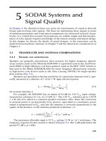
Infrasound is a longitudinal pressure wave [1–4]. The characteristics of these waves are
similar to audible acoustic waves but the frequency range is far below what the human
ear can detect. The typical frequenc y ran ge is from 0.01 to 10 Hz (Figure 3 .1). Natur e is an
incredible creator of infrasonic signals that can emanate from sources such as volcano
eruptions, earthquakes, severe weather, tsunamis, meteors (bolides), gravity waves,
microbaroms (infrasound radiated from ocean waves), surf, mountain ranges (mountain
associated waves), avalanches, and auroral waves to name a few. Infrasound can also
result from man-made events such as mining blasts, the space shuttle, high-speed aircraft,
artillery fire, rockets, vehicles, and nuclear events. Because of relatively low atmospheric

absorption at low frequencies, infrasound waves can travel long distances in the Earth’s
atmosphere and can be detected with sensitive ground-based sensors.
An integral part of the comprehensive nuclear test ban treaty (CTBT) international
monitoring syst em (IMS) is an infrasound network system [3]. The goal is to have 60
ß 2007 by Taylor & Francis Group, LLC.
infrasound arrays operational worldwide over the next several years. The main objective
of the infrasound monitoring system is the detection and verification, localization, and
classification of nuclear explosions as well as other infrasonic signals-of-interest (SOI).
Detection refers to the problem of detecting an SOI in the presence of all other unwanted
sources and noises. Localization deals with finding the origin of a source, and classifica-
tion deals with the discrimination of different infrasound events of interest. This chapter
concentrates on the classification part only.
3.2 Neural Networks for Infrasound Classification
Humans excel at the task of classifying patterns. We all perform this task on a daily basis.
Do we wear the checkered or the striped shirt today? For example, we will probably select
from a group of checkered shirts versus a group of striped shirts. The grouping process is
carried out (probably at a near subconscious level) by our ability to discriminate among all
shirts in our closet and we group the striped ones in the striped class and the checkered ones
in the checkered class (that is, without physically moving them around in the closet, only in
our minds). However, if the closet is dimly lit, this creates a potential problem and
diminishes our ability to make the right selection (that is, we are working in a ‘‘noisy’’
environment). In the case of using an artificial neural network for classification of patterns
(or various ‘‘events’’) the same problem exists with noise. Noise is everywhere.
In general, a common problem associated with event classification (or detection and
localization for that matter) is environmental noise. In the in frasound problem, many
times the distance between the source and the sensors is relatively large (as opposed to
region infrasonic phenomena). Increases in the distance between sources and sensors
heighten the environmental dependence of the signals. For example, the signal of an
infrasonic event that takes place near an ocean may have significantly different charac-
teristics as compared to the same event that occurs in a desert. A major contributor of

noise for the signal near an ocean is microbaroms. As mentioned above, microbaroms are
generated in the air from larg e ocean waves. One important characteristic of neural
networks is their noise rejection capability [5]. This, and several other attributes, makes
them highly desirable to use as classifiers.
FIGURE 3.1
Infrasound spectrum.
0.01 0.03 0.1 0.2 1.0 10.0
1 Megaton
yield
Volcano
events
Micro-
baroms
1 Kiloton
yield
Impulsive
events
Gravity
waves
Mountain
associated
waves
Bolide
0.01 0.03 0.1 0.2 1.0 10.0
Hz
Hz
ß 2007 by Taylor & Francis Group, LLC.
3.3 Details of the Approach
Our approach of classifying infrasound events is based on a parallel bank neural network
structure [6–10]. The basic architecture is shown in Figure 3.2. There are several reasons for

using such an architecture; however, one very important advantage of dedicating one
module to perform the classification of one event class is that the architecture is fault
tolerant (i.e., if one module fails, the rest of the individual classifiers will continue to
function). However, the overall performance of the classifier is enhanced when the parallel
bank neural network classifier (PBNNC) architecture is used. Individual banks (or mod-
ules) within the classifier architecture are radial basis function neural networks (RBF NNs)
[5]. Also, each classifier has its own dedicated preprocessor. Customized feature vectors are
computed optimally for each classifier and are based on cepstral coefficients and a subset of
their associated derivatives (differences) [11]. This will be explained in detail later. The
different neural modules are trained to classify one and only one class; however, for the
requisite module responsible for one of the classes, it is also trained not to recognize all
other classes (negative reinforcement). During the training process, the output is set to a ‘‘1’’
for a correct class and a ‘‘0’’ for all the other signals associated with all the other classes.
When the training process is complete the final output thresholds will be set to an optimal
value based on a three-dimensional receiver operating characteristic (3-D ROC) curve for
each one of the neural modules (see Figure 3.2).
Infrasound
signal
Pre-processor 1
Pre-processor 2
Pre-processor 3
Pre-processor 4
Infrasound class 1
neural network
Infrasound class 2
neural network
Infrasound class 3
neural network
Infrasound class 4
neural network

Infrasound class 5
neural network
Infrasound class 6
neural network
Pre-processor 5
Pre-processor 6
Optimum threshold
set by ROC curve
Optimum threshold
set by ROC curve
Optimum threshold
set by ROC curve
Optimum threshold
set by ROC curve
Optimum threshold
set by ROC curve
Optimum threshold
set by ROC curve
1
0
1
0
1
0
1
0
1
0
1
0

FIGURE 3.2
Basic parallel bank neural network classifier (PBNNC) architecture.
ß 2007 by Taylor & Francis Group, LLC.
3.3. 1 Infras ound Data Colle cted fo r Traini ng and Testing
The data used for train ing and testing the individual network s are obt ained from mult iple
infr asound arr ays locate d in differen t geogr aphi cal regions with differen t geome tries. The
six infr asound classes used in this study are shown in Table 3.1, and the vari ous arr ay
geomet ries are shown in Figure 3.3(a) through Figu re 3.3(e) [12,13 ]. Table 3.2 sho ws the
vario us classes, along with the arr ay numbe rs where the data were collected , and the
ass ociated sa mpling freque ncies.
3.3. 2 Radial Basis Fu nction Neur al Networ ks
As previousl y mentioned , eac h of the neural netw ork modu les in Figure 3.2 is an RBF NN.
A brief overview of RBF NNs will be given here. Thi s is not meant to be an exhaustive
discourse on the subject, but only an introduction to the subject. More details can be found
in Refs. [5,14].
Earlier work on the RBF NN was carried out for handling multivariate interpolation
problems [15,16]. However, more recently they have been used for probability density
estimation [17–19] and approximations of smooth multivariate functions [20]. In prin-
ciple, the RBF NN makes adjustments of its weights so that the error between the actual
and the desired responses is minimized relative to an optimization criterion through a
defined learning algorithm [5]. Once trained, the networ k performs the interp olation in
the output vector space, thus the generalization property.
Radial basis functions are one type of positive-definite kernels that are extensively used
for multivariate interpolation and approximation. Radial basis functions can be used for
problems of any dimension, and the smoothness of the interpolants can be achieved to
any desirable extent. Moreover, the structures of the interpolants are very simple. How-
ever, there are several challenges that go alon g with the aforementioned attributes of RBF
NNs. For example, many times an ill-conditioned linear system must be solved, and the
complexity of both time and space increases with the number of interpolation points. But
these types of problems can be overcome.

The interpolation problem may be formulated as follows. Assume M distinct data
points X ¼ {x
1
, ,x
M
}. Also assume the data set is bounded in a region V (for a specific
class). Each observed data point x 2 R
u
(u corresponds to the dimension of the input
space) may correspond to some function of x. Mathematically, the interpolation problem
may be stated as follows. Given a set of M points, i.e., {x
i
2 R
u
ji ¼ 1, 2, . . . , M} and a
corresponding set of M real numbers {d
i
2 R ji ¼ 1, 2, . . . , M} (desired outputs or the
targets), find a function F:R
M
! R that satisfies the interpolation condition
F(x
i
) ¼ d
i
, i ¼ 1, 2, , M (3:1)
TABLE 3.1
Infrasound Classes Used for Training and Testing
Class Number Event No. SOI (n ¼574)
No. SOI Used for

Training (n ¼351)
No. SOI Used for
Testing (n ¼223)
1 Vehicle 8 4 4
2 Artillery fire (ARTY) 264 132 132
3 Jet 12 8 4
4 Missile 24 16 8
5 Rocket 70 45 25
6 Shuttle 196 146 50
ß 2007 by Taylor & Francis Group, LLC.
−20
YDIS, m
XDIS, m
30
20
10
−10
−10 10 20 30−20−30−40
−20
−30
Sensor 1
(0.0, 0.0)
Sensor
2
(−18.6, −7.5)
Sensor
4
(15.3, −12.7)
Array BP1
Sensor

3
(3.1, 19.9)
YDIS, m
XDIS, m
30
20
10
−10
−10
10 20 30
−20−30−40
−20
−30
Sensor 1
(0.0, 0.0)
Sensor
5
(−19.8, 0.0)
Sensor
2
(−1.3, −19.9)
Sensor
4
(19.8, −0.1)
Array BP2
Sensor
3
(0.7, 20.1)
YDIS, m
XDIS, m

30
20
10
−10
−10 10 20 30 40−20−30−40
−20
−30
Sensor 1
(0.0, 0.0)
Sensor
2
(−22.0, 10.0)
Sensor
4
(45.0, −8.0)
Array K8201
Sensor
3
(28.0, −21.0)
YDIS, m
XDIS, m
30
20
10
−10
−10 10 20 30−30−40
−20
−30
Sensor 1
(0.0, 0.0)

Sensor
2
(−20.1, 0.0)
Sensor
4
(20.3, 0.5)
Array K8202
Sensor
3
(0.0, 20.2)
YDIS, m
XDIS, m
30
20
10
−10
−10
10 20 30
−20−30−40
−20
−30
Sensor 1
(0.0, 0.0)
Sensor
2
(−12.3, −15.8)
Sensor 4

(14.1, −14.1)
Arra

y
K8203
Sensor
3
(1.1, 20.0)
(a) (b)
(c)
(e)
(d)
FIGURE 3.3
Five different array geometries.
ß 2007 by Taylor & Francis Group, LLC.
Thus , all the point s must pass thr ough the interpol ating sur face. A radial basis func tion
may be a special inte rpolating func tion of the form
F( x)¼
X
M
i¼ 1
w
i
f
i
( xÀ x
i
kk
2
)(3:2)
wh ere f (
.
) is kno wn as the radial basis functi on andk

.
k
2
deno tes the Euc lidean norm . In
gene ral, the data point s x
i
are the center s of the radial ba sis func tions and are frequ ently
writt en as c
i
.
One of the problem s encounter ed when attempti ng to fit a func tion to da ta point s is
over -fitting of the data, that is, the value of M is too large. Howeve r, general ly speaking,
this is less a problem the RBF NN that it is with , for example , a multi-l ayer per ceptron
train ed by backpro pagation [5]. The RBF NN is attemptin g to constru ct the hype rspace for
a particul ar pro blem wh en given a limited number of da ta point s.
Let us take another point of view concer ning how an RBF NN per form s its constr uction
of a hype rsurface . Regul arization theo ry [5,14] is applied to the constr uction of the
hype rsurface . A geomet rical explanati on follo ws.
Consi der a set of input data obt ained from sever al events from a single cl ass. The inp ut
data may be from temp oral sign als or defined features obt ained from thes e sign als usin g
an appropriate transformation. The input data would be transformed by a nonlinear
function in the hidd en layer of the RBF NN. Each event would then correspond to a
point in the featu re spac e. Figure 3.4 depicts a two- dimensi onal (2-D) feature set, that is,
the dimension of the output of the hidden layer in the RBF NN is two. In Figure 3.4, ‘‘(a)’’,
‘‘(b)’’, and ‘‘(c)’’ correspond to three separate events. The purpose here is to construct a
surface (shown by the dotted line in Figure 3.4) such that the dotted region encompasses
events of the same class. If the RBF network is to classify four different classes, there must
be four different regions (four dotted contours), one for each class. Ideally, each of these
regions should be separate with no overlap. However, because there is always a limited
amount of observed data, perfect reconstruction of the hyperspace is not possible and it is

inevitable that overlap will occur.
To overcome this problem it is necessary to incorporate global information from V (i.e.,
the class space) in approximating the unknown hypersp ace. One choice is to introduce a
smoothness constraint on the targets. Mathematical details will not be given here, but for
an in-depth development see Refs. [5,14].
Let us now turn our attention to the actual RBF NN architecture and how the network
is trained. In its basic form, the RBF NN has three layers: an input layer, one hidden
TABLE 3.2
Array Numbers Associated with the Event Classes and the Sampling Frequencies Used to Collect
the Data
Class Number Event Array Sampling Frequency, Hz
1 Vehicle K8201 100
2 Artillery fire (ARTY)
(K8201: Sites 1 and 2)
K8201; K8203 (K8201: Sites 1 and 100;
Sites 2 and 50); 50
3 Jet K8201 50
4 Missile K8201; K8203 50; 50
5 Rocket BP1; BP2 100; 100
6 Shuttle BP2; BP103
a
100; 50
a
Array geometry not available.
ß 2007 by Taylor & Francis Group, LLC.
layer, and one output layer. Referring to Figure 3.5, the source nodes (or the input
components) make up the input layer. The hidden layer performs a nonlinear trans-
formation (i.e., the radial basis functions residing in the hidden layer perform this
transformation) of the input to the network and is generally of a higher dimension than
the input. This nonlinear transformation of the input in the hidden layer may be viewed

as a basis for the construction of the input in the transformed space. Thus, the term radial
basis function.
In Figure 3.5, the output of the RBF NN (i.e., at the output layer) is calculated
according to
y
i
¼ f
i
(x) ¼
X
N
k¼1
w
ik
f
k
(x,c
k
) ¼
X
N
k¼1
w
ik
f
k
( x À c
k
kk
2

), i ¼ 1, 2, , m (no: outputs) (3:3)
where x 2 R
uÂ1
is the input vector, f
k
(
.
) is a (RBF) function that maps R
þ
(set of all
positive real numbers) to R (field of real numbers), k
.
k
2
denotes the Euclidean norm, w
ik
are the weights in the output layer, N is the number of neurons in the hidden layer, and c
k
2 R
uÂ1
are the RBF centers that are selected based on the input vector space. The
Euclidean distance between the center of each neuron in the hidden layer and the input
to the network is computed. The output of the neuron in a hidden layer is a nonlinear
(a)
(b)
(c)
Feature 1
Feature 2
FIGURE 3.4
Example of a two-dimensional feature set.

f
1
f
2
f
N
W
T

∈ ℜ
m × N
Σ
Σ
y
1
y
m
x
1
x
2
x
3
x
u
Input layer Hidden layer Output layer
FIGURE 3.5
RBF NN architecture.
ß 2007 by Taylor & Francis Group, LLC.
func tion of this dista nce, and the output of the network is compu ted as a wei ghted sum of

the hidde n layer outpu ts.
The func tional form of the radial ba sis func tion, f
k
(
.
), can be any of the follow ing:
.
Line ar func tion: f( x)¼ x
.
Cubi c appr oximatio n: f (x)¼ x
3
.
Thin- plate-s pline function: f (x)¼ x
2
ln(x)
.
Gaus sian function : f (x)¼ exp(À x
2
/s
2
)
.
Mult i-quadrat ic functi on: f ( x)¼
ffiffiffiffiffiffiffiffiffiffiffiffiffiffiffiffi
x
2
þs
2
p
.

Inv erse multi-qu adratic function : f (x)¼ 1=(
ffiffiffiffiffiffiffiffiffiffiffiffiffiffiffiffi
x
2
þs
2
p
)
The parameter s contr ols the ‘‘width ’’ of the RBF and is common ly referr ed to as the
spre ad par ameter. In man y pr actical appl ications the Gaus sian RBF is used. The center s,
c
k
, of the Gau ssian func tions are points used to per form a sampl ing of the inp ut vector
spac e. In general , the center s form a subset of the inp ut data.
3. 4 D ata P reproc essi ng
3.4. 1 Noise Filtering
Microb aroms, a s pre viousl y def ined, are a persisten tly pres ent sour ce of noise that
resides in most collected infr asound sign als [21–23 ]. Mi crobarom s are a clas s of infr asonic
sign als charact eriz ed by narrow-b and, nearly sinu soidal wavef orms, with a period
bet ween 6 and 8 sec . These signal s can be gene rated by marin e sto rms through a non-
linear inte raction of surfac e waves [24]. The freque ncy conten t of the microbar oms often
coinci des with that of small-yi eld nuclea r ex plosions. This co uld be bothersome in man y
appli cations; howev er, simple band-pass filtering can allevi ate the pro blem in man y
case s. The refore, a band-pass filter with a pass band betwee n 1 and 49 Hz (for signal s
samp led at 100 Hz) is used here to elimi nate the effects of the microb aroms. Figure 3.6
shows how band-pass filteri ng can be used to elimina te the mi crobarom s problem .
3.4. 2 Featur e E xtractio n Process
Dep icted in eac h of the six graphs in Figure 3.7 is a collectio n of eight sign als from
each cl ass, that is, y
ij

(t ) for i¼ 1, 2, . . . , 6 (classe s) and j¼ 1, 2, . . . , 8 (num ber of sign als)
(see Ta ble 3.1 for total number of signals in each class). A feature extra ction proces s is
desired that wil l captu re the salient features of the sign als in each class and at the same
time be invarian t relative to the arr ay geome try, the geog raphica l locat ion of the array , the
samp ling frequenc y, and the leng th of the time window . The overall per formance of
the cl assifier is co ntingen t on the data that is used to train the neural netw ork in each of
the six modu les shown in Figure 3.2. Moreo ver, the neu ral netw ork’s ability to distinguish
between the various events (presented the neural networks as feature vectors) is the
distinctiveness of the features between the classes. However, within each class it is
desirable to have the feature vectors as similar to each other as possible.
There are two major questions to be answered: (1) What will cause the signals in one
class to have markedly different characteristics? (2) What can be done to minimize these
ß 2007 by Taylor & Francis Group, LLC.
differen ces and achieve uni formit y with in a class and distin ctive ly dif ferent featu re vector
charact eristic s between class es?
The answer to the first questi on is quite simple—n oise. This can be noise as sociated
with the sensors, the data acquis ition equip ment, or other unwa nted sign als that are not
of interest. The answ er to the sec ond question is also quite sim ple (once you know the
answ er)—using a feature extra ction process ba sed on compu ted cepst ral co efficients and
a subset of thei r assoc iated der ivatives (di fferences ) [10,11 ,25 –28].
As me ntioned in Secti on 3.3, each cl assifier has its own dedicat ed pre process or (see
Figure 3.2). Customi zed feature vec tors are compute d optim ally for each clas sifier (or
neural module) and are based on the aforem entio ned cepst ral coefficie nts and a subset of
their associa ted deriva tives (or differen ces). The pr eprocessin g proce dure is as follow s.
Each time-do main signal is first norm alized and then its mean value is co mpute d and
remove d. Next , the power spect ral dens ity (P SD) is calcu lated for each signal, whic h is a
mixtur e of the desire d comp onent and possi bly other unwa nted signal s and noise.
Therefor e, when the PSDs are comp uted for a set of signal s in a defin ed class there will
be spect ral compo nents ass ociate d wi th noise and ot her unwa nted signal s that need to be
suppres sed. This can be systemati cally accomp lished by first compu ting the av erage PSD

(i.e., PSD
avg
) over the suite of PSDs for a particul ar class . The spect ral co mponent s are
define d as m
i
for i¼ 1, 2, . . . for PSD
avg
. The max imum spect ral compo nent, m
max
,of
PSD
avg
is then deter mined. This is consi dered the dominan t spectral comp onent wi thin a
particul ar cl ass and its value is used to supp ress selected comp onents in the res ident PSDs
for any particu lar cl ass according to the follo wing:
if m

i
>«
1
m
max
(typ ically «
1
¼ 0: 001)
then m
i
m
i
else «

2
m
i
(typically «
2
¼ 0:00001)
1.5
0.5
0
0 500
Time samples
Before filtering
Amplitude
1000
–0.5
1
1
0.0
–0.5
0 500
Time samples
After filtering
Amplitude
1000
–1
0.5
Before filtering
8
6
4

2
0
–50 0
Frequency (Hz)Frequency (Hz)
After filtering
Magnitude
50
400
300
200
100
0
–50 0
Magnitude
50
FIGURE 3.6
Results of band-pass filtering to eliminate the effects of microbaroms (an artillery signal).
ß 2007 by Taylor & Francis Group, LLC.
To some extent, this will minimize the effects of any unwanted components that may
reside in the signals and at the same time minimize the effects of noise. However, another
step can be taken to further minimize the effects of any unwanted signals and noise that
may reside in the data. This is based on a minimum variance criterion applied to the
spectral components of the PSDs in a particular class after the previously described step is
completed. The second step is carried out by taking the first 90% of the spectral compon-
ents that are rank-ordered according to the smallest variance. The rest of the components
Raw time-domain 8 signals for vehicle
Amplitude
0.8
0.6
0.4

0.2
–0.2
–0.4
–0.6
0 100 200 300 400
Time (sec)
500 600 700
0
Raw time-domain 8 signals for missile
Amplitude
2
1.5
1
0.5
–0.5
–1
–1.5
–2
–2.5
–3
0 1000 2000 3000 4000
Time (sec)
5000 6000 7000 8000
0
Raw time-domain 8 signals for artillery
Amplitude
1.8
1.6
1.4
1.2

0.6
0.8
0.4
0.2
0
0 50 100 150 200
Time (sec)
250 300 350
1
Raw time-domain 8 signals for rocket
Amplitude
0.7
0.6
0.5
0.4
0.3
0.2
0.1
0
0 200 400 600 800
Time (sec)
1000 1200 1400 1600
Vehicle class
Missile class
Artillery class
Rocket class
(a)
(b)
(d)
(c)

Raw time-domain 8 signals for jet
Amplitude
1.4
1.2
1
0.8
0.4
0.2
0
–0.4
–0.2
0 500 1000 1500 25002000
Time (sec)
3000 3500 4000 4500
0.6
Raw time-domain 8 signals for shuttle
Amplitude
1
0.9
0.8
0.7
0.5
0.4
0.3
0.2
0.1
0
100
200 300 400
Time (sec)

500 600 700 800 900 1000
0.6
Jet class
Shuttle class
(e) (f)
FIGURE 3.7 (See color insert following page 178.)
Infrasound signals for six classes.
ß 2007 by Taylor & Francis Group, LLC.
in the power spectral densities within a particular class are set to a small value, that is, «
3
(typically 0.00001). Therefore, the number of spectral components greater than «
3
will
dictate the number of components in the cepstral domai n (i.e., the number of cepstral
coefficients and associated differences). Depending on the class, the number of coeffi-
cients and differences will vary. For example, in the simulations that were run, the largest
number of components was 2401 (artillery class) and the smallest number was 543
(vehicle class). Next, the mel-frequency scaling step is carried out with defined values
for a and b [10], then the inverse discrete cosine transform is taken and the derivatives
(differences) are computed.
From this set of computed cepstral coefficients and differences, it is desired to select
those components that will constitute a feature vector that is consistent within a particular
class. That is, there is minimal variation among similar components across the suite of
feature vectors. So the approach taken here is to think in terms of minimum variance of
these similar components within the feature set.
Recall, the time-domain infrasound signals are assumed to be band-pass filtered to
remove any effects of microbaroms as described previously. For each discrete-time
infrasound signal, y(k), where k is the discrete time index (an integer), the specific
preprocessing steps are (dropping the time dependence k):
(1) Normalize (i.e., divide each sample in the signal y(k) by the absolute value of

the maximum amplitude, jy
max
j, and also divide by the square root of the
computed variance of the signal, s
y
2
, and then remove the mean:
y y={jy
max
j,s
y
}(3:4)
y y À mean(y)(3:5)
(2) Compute the PSD, S
yy
(k
v
), of the signal y:
S
yy
(k
v
) ¼
X
1
t¼0
R
yy
(t)e
Àjk

v
t
(3:6)
where R
yy
() is the autocorrelation of the infrasound signal y.
(3) Find the average of the entire set of PSDs in the class, i.e., PSD
avg
(4) Retain only those spectral components whose contributions will maximize the
overall performance of the global classifier:
if m
i
> «
1
m
max
(typically «
1
¼ 0:001)
then m
i
m
i
else «
2
m
i
(typically «
2
¼ 0:00001)

(5) Compute variances of the components selected in Step (4). Then take the first
90% of the spectral components that are rank-ordered according to the smallest
variance. Set the remaining components to a small value, i.e., «
3
(typically
0.00001).
(6) Apply mel-frequency scaling to S
yy
(k
v
):
S
mel
(k
v
) ¼ a log
e
½bS
yy
(k
v
) (3:7)
where a ¼ 11.25, b ¼ 0.03.
ß 2007 by Taylor & Francis Group, LLC.
(7) Take the inverse discr ete cosin e transform :
x
mel
(n )¼
1
n

X
NÀ 1
k
v
¼ 0
S
m
( k
v
) cos(2 pk
v
n=N ) for n¼ 0, 1, 2, , NÀ 1(3:8)
(8) Take the consecu tive differen ces of the sequen ce x
mel
( n) to obt ain x
0
mel
( n).
(9) Concate nate the sequen ce of differe nces, x
0
mel
(n), with the ce pstral coefficie nt
sequen ce, x
mel
( n), to form the augm ented sequen ce:
x
a
mel
¼ [ x
0

mel
( i)j x
mel
(j )] (3 :9)
wh ere i and j are det ermined exp erimenta lly. As mentio ned previous ly, i¼ 400
and j¼ 600.
(10) Take the abs olute value of the elemen ts in the sequen ce x
mel
a
yiel ding:
x
a
mel
,abs
¼jx
a
mel
j (3 :10)
(11) Take the log
e
of x
a
mel
,abs
from the previous step to give:
x
a
mel
,abs,log
¼ log

e
½ x
a
mel
, abs
 (3 :11)
Appl ying this 11-ste p feature extra ction proce ss to the infr asound signals in the six
differe nt cl asses resu lts in the featu re vectors shown in Figure 3.8. The leng th of each
feature vector is 34. This wi ll be exp lained in the next section. If these sets of feature
vecto rs are compare d to thei r tim e-domain sign al co unterpar ts (see Figure 3.7), it is
obviou s that the feature extractio n proce ss pro duces featu re vecto rs that are mu ch more
consi stent than the tim e-domain signals. More over, comparin g the feature vectors be-
tween classes re veals that the dif ferent sets of feature vectors are marked ly distinct. This
shou ld resu lt in im prove d cl assificati on per forma nce.
3.4. 3 Usefu l Defini tions
Before we go on, let us def ine som e useful qua ntities that apply to the assessm ent of
performance for classifiers. The confusion matrix [29] for a two-class classifier is shown in
Tab le 3.3.
In Table 3.3 we have the following:
p: number of correct predictions that an occurrence is positive
q: number of incorrect predictions that an occurrence is positive
r: number of incorre ct of predictions that an occurrence is negative
s: number of correct predictions that an occurrence is negative
With this, the correct classification rate (CCR) is defined as
CCR ¼
No: correct predictions À No: Â classifications
No: predictions
¼
p þ s À No: multiple classifications
p þ q þ r þ s

(3:12)
ß 2007 by Taylor & Francis Group, LLC.
Multiple classifications refer to more than one of the neural modules showing a ‘‘posi-
tive’’ at the output of the RBF NN indicating that the input to the global classifier belongs
to more than one class (whether this is true or not). So there could be double, triple,
quadruple, etc., classifications for one event.
The accuracy (ACC) is given by
ACC ¼
No: correct predictions
No predictions
¼
p þ s
p þ q þ r þ s
(3:13)
(a) Feature set for vehicle (b) Feature set for missile
(c) Feature set for artillery fire
(d) Feature set for rocket
(e) Feature set for jet
(f) Feature set for shuttle
10
9
8
7
6
5
4
3
5 101520
Feature number
Amplitude

Amplitude
Amplitude
Amplitude
Amplitude
Amplitude
25 30
10
9
8
7
6
5
4
3
5101520
Feature number
25 30
10
9
8
7
6
5
4
3
5101520
Feature number
25 30
10
9

8
7
6
5
4
3
5101520
Feature number
25 30
10
9
8
7
6
5
4
3
5 101520
Feature number
25 30
10
9
8
7
6
5
4
3
5
10 15 20

Feature number
25 30
FIGURE 3.8 (See color insert following page 178.)
Infrasound signals for six class different classes.
ß 2007 by Taylor & Francis Group, LLC.
As seen from Equa tion 3.12 and Equation 3.13, if mu ltiple class ifications occur, the CC R is
a more co nservativ e per formance meas ure than the ACC. However , if no multiple
clas sificatio ns oc cur, the CCR¼ AC C.
The true posi tive (TP ) rate is the propor tion of positive cases that are co rrectly iden ti-
fied. This is compu ted usin g
TP¼
p
pþ q
(3 :14)
The false posi tive (FP) rate is the pro portion of negative case s that are incorre ctly
clas sified a s posi tive occu rrences. This is compute d using
FP¼
r
rþ s
(3 :15)
3.4. 4 Selec tion Process for the Optim al Num ber of F eature Vec tor Comp onents
From the set of computed cepstral coefficients an d d iff eren ce s gener a ted using th e
feature extractio n pro cess given a bove, a n optimal subset of these is desired that wi ll
constitute the feature vect ors used t o train an d t est t he PBNNC sh own in Fi gure 3.2.
The optimal su bset (i.e., the optimal feature v ector length) is dete rmined by taking a
minimum v ariance a pp roach. Sp ecificall y, a 3-D graph i s generated that plo ts the
performance; that is, CCR versus th e RBF NN spread parameter and the f eature vector
n umber (see Figu re 3.9) . From th is graph , m ean v alues a nd varian ces a re com puted
across th e r ange of spread param eter s f or each o f th e def ine d nu mber of c om pon ents in
the f eature vector. The selection criterion is define d a s simu ltaneously maximizing

themeanandatthesametimeminimizingthe varian ce. Maximization of t he mean
ensures m aximum performance; that is, m axi mizing the CCR and at the same t ime
minimizing the v ariance t o m inimize v ariati on in the f eature set within each of the
classes. The output threshold a t each o f t he ne u ral modules (i.e., t he outp ut of the single
output neuron of each RBF N N) is set optimally accordi ng t o a 3-D RO C curve. This wi ll
be explained ne xt.
Figure 3.10 shows the two plots used to det ermine the max imum mean and the
minimu m varian ce. The table insert betwee n the two graphs shows that even though
the mean val ue for 40 elemen ts in the feature vector is (sl ightly) larger than that for
34 ele ments, the varian ce for 40 is nearly three time s that for 34 elemen ts. The refore, a
len gth of 34 elemen ts fo r the feature vectors is the best choice .
3.4. 5 Optim al Output Thr eshold Valu es and 3-D ROC Curves
At the output of the RBF NN for eac h of the six ne ural mod ules, there is a sin gle output
neu ron with har d-limi ting binary val ues used duri ng the train ing proce ss (see Figure 3.2).
Afte r train ing, to determi ne whet her a particul ar SO I belongs to on e of the six classes, the
TABLE 3.3
Confusion Matrix for a Two-Class Classifier
Predicted Value
Actual Value Positive Negative
Positive pq
Negative rs
ß 2007 by Taylor & Francis Group, LLC.
thresho ld value of the output neurons is optim ally set accordi ng to an ROC curve [30–32 ]
for that individual neural modu le (i.e., one particu lar class ). Before an ex planatio n of the
3-D ROC cu rve is given, let us first revi ew 2-D ROC curves and see how they are used to
optim ally set threshold values.
An ROC curve is a plot of the TP rate versu s the FP rate, or the sensit ivity versu s
(1 – speci ficity); a sa mple ROC curve is shown in Figure 3.11. The optim al thr eshold
value correspo nds to a point nearest the ideal point (0, 1) on the grap h. The point (0, 1)
is consi dered ideal becau se in this case there would be no false positi ves and onl y true

positive s. Ho wever, bec ause of noise and ot her undes irable effects in the da ta, the
point cl osest to the (0, 1) point (i.e., the minimum Euclide an dista nce) is the best that
we can do. This will then dictate the optim al thresho ld val ue to be used at the output of
the RBF NN .
Since there are six classifier s, that is, six neural modules in the global clas sifier, six ROC
curves must be gene rated. Ho wever, usin g 2-D ROC curves to set the thresh olds at the
outputs of the six RBF NN clas sifiers wi ll not res ult in optim al thresho lds. Thi s is bec ause
miscla ssificati ons are not taken into accou nt wh en sett ing the thresh old for a parti cular
neural mod ule that is res ponsible for classifying a particul ar set of infrasoun d signal s.
Reca ll that one neural mo dule is assoc iated with one infras onic clas s, and each neu ral
modu le acts as its own classifier . The refore, it is nece ssary to accou nt for the misclas sifica-
tions that can occur and this can be accompli shed by adding a third dimensi on to the ROC
curve. When the misclass ificatio ns are taken into accou nt the (0, 1, 0) point now become s
the optimal point, and the smallest Euclidean distance to this point is directly related to
Performance (CCR) 3-D plot using ROC curve
100
80
60
40
20
0
2.5
2.0
1.5
1.0
0.5
0.1
10
20
30

40
50
60
Feature number
Spread parameter
CCR (%)
Compute mean
and variance
Compute mean
and variance
Compute mean
and variance
Compute mean
and variance
Compute mean
and variance
FIGURE 3.9 (See color insert following page 178.)
Performance plot used to determine the optimal number components in the feature vector. Ill conditioning
occurs for the feature number less than 10, and for the feature number greater than 60, the CCR dramatically
declines.
ß 2007 by Taylor & Francis Group, LLC.
10 15 20 25 30 35 40 45 50 55 60
40
45
50
55
60
65
70
Feature number

10 15 20 25 30 35 40 45 50 55 60
0
50
100
150
200
250
300
350
400
450
500
Feature number
34 Features
Performance meanPerformance variance
34 Features
Feature number
Mean Variance
34 66.9596 47.9553
40 69.2735
122.834
FIGURE 3.10
Performance means and performance variances versus feature number used to determine the optimal length
of the feature vector.
ß 2007 by Taylor & Francis Group, LLC.
the optim al thresho ld value for each neu ral mod ule. Figure 3.12 shows the six 3-D ROC
curves ass ociated with the cl assifiers .
3.5 Simul ation R esults
The fou r basic parameter s that are to be optimized in the proce ss of training the neu ral
netw ork cl assifier (i.e ., the bank of six RBF NN s) are the RBF NN spr ead paramete rs, the

output thresho lds of each neural modu le, the combinat ion of 34 compo nents in the fe ature
vectors for each class (note again in Figure 3.2, each neural mod ule has its own cus tom
prepro cessor ) a nd of cours e the res ulting weights of each RBF NN . The MA TLAB neu ral
netw orks toolbox was used to desig n the six RBF NN s [33] .
Table 3.1 sho ws the specific clas ses and the assoc iated number of sign als used to
train and test the RBF NNs. Of the 57 4 infras ound sign als, 351 were used for train ing
the remain ing 2 23 were used for testing . The criterio n used to divide the data bet ween
the training a nd te sting sets was to maint ain indepen dence. Henc e, the four array
signal s from any one even t are always kept together, eithe r in the train ing set or the
test set.
After the optim al number compo nents for each feature vector was determi ned, i.e., 34
elemen ts, and the optim al combi nation of the 34 comp onents for each prepro cessor, the
optim al RBF spre ad parameter s are det ermined along with the optim al thresho ld value
(the six graphs in Figure 3.12 were used for this purpose). For both the RBF spread
paramete rs and the output thresho lds, the selection criterio n is based on max imiz ing
the CCR of the local netw ork and the over all (globa l) classifier CCR.
The RBF spre ad paramete r and the outpu t thr eshold for each neural mod ule was
determi ned one by one by fixing the spread parameter , i.e., s, for all other neural mod ules
to 0.3, and hold ing the thresh old value at 0.5. Once the first neural mod ule’s spre ad
0 0.1 0.2 0.3 0.4 0.5
FP (1 − specificity)
TP (sensitivity)
0.6 0.7 0.8 0.9 1
1
0.9
0.8
0.7
0.6
0.5
0.4

Minimum
Euclidean
distance
ROC curve
FIGURE 3.11
Example ROC curve.
ß 2007 by Taylor & Francis Group, LLC.
parame ter and threshold is determine d, then the spre ad par ameter and output thresho ld
of the secon d neural mod ule is comp uted wh ile holding all ot her neu ral modu les’ (except
the first one ) spre ad parameter s and output thresholds fixed at 0.3 and 0.5, resp ectively.
Tab le 3.4 gives the final val ues of the spre ad par ameter and the outpu t thresho ld for the
global classifier . Figure 3.13 shows the cl assifier arch itecture with the final values indi-
cated for the RBF NN spre ad parameter s and the output thresh olds.
Tab le 3.5 shows the confusio n matr ix for the six-classi fier. Concentr ating on the 6Â 6
por tion of the matr ix for eac h of the define d clas ses, the diagon al elemen ts correspond to
0
0.2
0.4
0.6
0.8
1
0.2
0.4
0.6
0.8
1
1.5
2
2.5
3

3.5
4
False positive
(a) ROC 3-D plot for vehicle
(c) ROC 3-D plot for artillery
(e) ROC 3-D plot for jet
(f) ROC 3-D plot for shuttle
(d) ROC 3-D plot for rocket
(b) ROC 3-D plot for missile
True positive
True positive
True positive
True positive
True positive
Misclassification
0
0.2
0.4
0.6
0.8
1
0
0.5
1
0
1
2
3
4
5

False positive
Misclassification
0
0.2
0.4
0.6
0.8
1
0.2
0.4
0.6
0.8
1
0
1
2
3
4
5
False positive
True positive
Misclassification
0
0.2
0.4
0.6
0.8
1
0
0.5

1
0
1
2
3
4
5
False positive
Misclassification
0
0.2
0.4
0.6
0.8
1
0
0.5
1
0
1
2
3
4
5
False positive
Misclassification
0
0.2
0.4
0.6

0.8
1
0
0.5
1
0
1
2
3
4
5
False positive
Misclassification
Artillery
Vehicle
Jet
Missile
Rocket
Shuttle
FIGURE 3.12
3-D ROC curves for the six classes.
ß 2007 by Taylor & Francis Group, LLC.
the correct predic tions. The trace of this 6Â6 matr ix divide d by the total numbe r of signal s
teste d (i.e ., 2 23) gives the accura cy of the global clas sifier. The formula for the accura cy is
given in Eq uation 3.13, and here ACC¼ 94.6% . The off-diagon al eleme nts ind icate the
miscl assificati ons that occu rred and those in parenthe ses indicate doubl e cl assificati ons
(i.e., the actual class was iden tified correc tly, but there was another one of the output
thresho lds for ano ther class that was exce eded). The off-diagon al elemen t that is in squa re
TABLE 3.4
Spread Parameter and Threshold of Six-Class Classifier

Spread Parameter Threshold Value True Positive False Positive
Vehicle 0.2 0.3144 0.5 0
Artillery 2.2 0.6770 0.9621 0.0330
Jet 0.3 0.6921 0.5 0
Missile 1.8 0.9221 1 0
Rocket 0.2 0.4446 0.9600 0.0202
Shuttle 0.3 0.6170 0.9600 0.0289
Infrasound
signal
Pre-processor 1
Infrasound class 1
neural network
Infrasound class 2
neural network
Infrasound class 3
neural network
Infrasound class 4
neural network
Infrasound class 5
neural network
Infrasound class 6
neural network
Pre-processor 2
Pre-processor 3
Pre-processor 4
Pre-processor 5
Pre-processor 6
Optimum threshold
set by ROC curve
(0.3144)

Optimum threshold
set by ROC curve
(0.6770)
Optimum threshold
set by ROC curve
(0.6921)
Optimum threshold
set by ROC curve
(0.9221)
Optimum threshold
set by ROC curve
(0.4446)
Optimum threshold
set by ROC curve
(0.6170)
s
1
= 0.2
s
2
= 2.2
s
3
= 0.3
s
4
= 1.8
s
5
= 0.2

s
6
= 0.3
1
0
1
0
1
0
1
0
1
0
1
0
FIGURE 3.13
Parallel bank neural network classifier architecture with the final values for the RBF spread parameters and
the output threshold values.
ß 2007 by Taylor & Francis Group, LLC.
bracke ts is a doub le misclas sificatio n, that is, this even t is misclas sified alon g with anoth er
mis classified event (th is is a shuttle event that is mi sclassif ied as bot h a ‘‘rock et’’ even t as
wel l as an ‘‘artill ery’’ event).
Tab le 3.6 shows the final global cl assifier results giving both the CC R (se e Equa tion
3.12) and the ACC (see Eq uation 3.13). Simul ations were also run usin g ‘‘bi-polar ’’
outpu ts inste ad of binary outputs. For the case of bi-polar outputs, the outpu t is boun d
bet weenÀ 1 andþ1 inste ad of 0 and 1. As can be seen from the tabl e, the binary case
yield ed the best result s. Final ly, Table 3.7 sho ws the resu lts for the case where the
thresh old level s on the outputs of the ind ividual RBF NNs are ignored and only the
outpu t with this large st value is taken as the ‘‘winn er,’’ that is, ‘‘winner- takes-al l’’; this is
consi dered to be the clas s that the inp ut SOI belongs to. It shou ld be noted that even

thoug h the CCR shows a hig her level of perform ance for the winne r-take s-all approach,
this is prob ably not a via ble method for classificati on. The reas on bein g that if there were
truly multiple even ts occurr ing simulta neously, they wo uld neve r be indicate d as such
usin g this approach.
TABLE 3.5
Confusion Matrix for the Six-Class Classifier
Predicted Value
Vehicle Artillery Jet Missile Rocket Shuttle Unclassified Total (223)
Vehicle 2 (1) 0 0 0 0 2 4
Artillery 0 127 0 0 0 0 5 132
Actual Jet 0 0 2 0 0 0 2 4
Value Missile 0 0 0 8 0 0 0 8
Rocket 0 0 0 0 24 (5) 1 25
Shuttle 0 (1)[1] 0 0 1(3) 48 1 50
TABLE 3.6
Six-Class Classification Result Using a Threshold Value for Each
Network
Performance Type Binary Outputs (%) Bi-Polar Outputs (%)
CCR 90.1 88.38
ACC 94.6 92.8
TABLE 3.7
Six-Class Classification Result Using ‘‘Winner-Takes-All’’
Performance Type Binary Method (%) Bi-Polar Method (%)
CCR 93.7 92.4
ACC 93.7 92.4
ß 2007 by Taylor & Francis Group, LLC.
3.6 Conclusions
Radial basis function neural networks were used to classify six different infrasound
events. The classifier was built with a parallel structure of neural mo dules that individu-
ally are responsible for classifying one and only one infrasound event, referred to as

PBNNC architecture. The overall accuracy of the classifier was found to be greater than
90%, using the CCR performance criterion. A feature extraction technique was employed
that had a major impact toward increasing the classification performance over most other
methods that have been tried in the past. Receiver operating characteristic curves were
also employed to optim ally set the output thresholds of the individual neural modules in
the PBNNC architecture. This also contributed to increased performance of the global
classifier. And finally, by optimizing the individual spread parameters of the RBF NN, the
overall classifier performance was increased.
Acknowledgments
The authors would like to thank Dr. Steve Tenney and Dr. Duong Tran-Luu from the
Army Research Laboratory for their support of this work. The authors also thank Dr.
Kamel Rekab, University of Missouri–Kansas City, and Mr. Young-Chan Lee, Florida
Institute of Technology, for their comments and insight.
References
1. Pierce, A.D., Acoustics: An Introduction to Its Physical Principles and Applications, Acoustical
Society of America Publications, Sewickley, PA, 1989.
2. Valentina, V.N., Microseismic and Infrasound Waves, Research Reports in Physics, Springer-
Verlag, New York, 1992.
3. National Research Council, Comprehensive Nuclear Test Ban Treaty Monitoring, National Academy
Press, Washington, DC, 1997.
4. Bedard, A.J. and Georges, T.M., Atmospheric infrasound, Physics Today, 53(3), 32–37, 2000.
5. Ham, F.M. and Kostanic, I., Principles of Neurocomputing for Science and Engineering, McGraw-
Hill, New York, 2001.
6. Torres, H.M. and Rufiner, H.L., Automatic speaker identification by means of mel cepstrum,
wavelets and wavelet packets, In Proc. 22nd Annu. EMBS Int. Conf., Chicago, IL, July 23–28, 2000,
pp. 978–981.
7. Foo, S.W. and Lim, E.G., Speaker recognition using adaptively boosted classifier, In Proc. The
IEEE Region 10th Int. Conf. Electr. Electron. Technol. (TENCON 2001), Singapore, Aug. 19–22, 2001,
pp. 442–446.
8. Moonasar, V. and Venayagamoorthy, G., A committee of neural networks for automatic speaker

recognition (ASR) systems, IJCNN, Vol. 4, Washington, DC, 2001, pp. 2936–2940.
9. Inal, M. and Fatihoglu, Y.S., Self-organizing map and associative memory model hybrid classifier
for speaker recognition, 6th Seminar on Neural Network Applications in Electrical Engineering,
NEUREL-2002, Belgrade, Yugoslavia, Sept. 26–28, 2002, pp. 71–74.
10. Ham, F.M., Rekab, K., Park, S., Acharyya, R., and Lee, Y C., Classification of infrasound
events using radial basis function neural networks, Special Session: Applications of learning
and data-driven methods to earth sciences and climate modeling, Proc. Int. Joint Conf. Neural
Networks, Montre
´
al, Que
´
bec, Canada, July 31–August 4, 2005, pp. 2649–2654.
ß 2007 by Taylor & Francis Group, LLC.
11. Mammone, R.J., Zhang, X., and Ramachandran, R.P., Robust speaker recognition: a feature-
based approach, IEEE Signal Process. Mag., 13(5), 58–71, 1996.
12. Noble, J., Tenney, S.M., Whitaker, R.W., and ReVelle, D.O., Event detection from small aper-
ture arrays, U.S. Army Research Laboratory and Los Alamos National Laboratory Report,
September 2002.
13. Tenney, S.M., Noble, J., Whitaker, R.W., and Sandoval, T., Infrasonic SCUD-B launch signatures,
U.S. Army Research Laboratory and Los Alamos National Laboratory Report, October 2003.
14. Haykin, S., Neural Networks: A Comprehensive Foundation, 2nd ed., Prentice-Hall, Upper Saddle
River, NJ, 1999.
15. Powell, M.J.D., Radial basis functions for multivariable interpolation: a review, IMA conference on
Algorithms for the Approximation of Function and Data, RMCS, Shrivenham, U.K., 1985, pp. 143–167.
16. Powell, M.J.D., Radial basis functions for multivariable interpolation: a review, Algorithms for the
Approximation of Function and Data, Mason, J.C. and Cox, M.G., Eds., Clarendon Press, Oxford,
U.K., 1987.
17. Parzen, E., On estimation of a probability density function and mode, Ann. Math. Stat., 33,
1065–1076, 1962.
18. Duda, R.O., and Hart, P.E., Pattern Classification and Scene Analysis, John Wiley & Sons, New

York, 1973.
19. Specht, D.F., Probabilistic neural networks, Neural Networks, 3(1), 109–118, 1990.
20. Poggio, T. and Girosi, F., A Theory of Networks for Approximation and Learning, A.I. Memo 1140,
MIT Press, Cambridge, MA, 1989.
21. Wilson, C.R. and Forbes, R.B., Infrasonic waves from Alaskan volcanic eruptions, J. Geophys.
Res., 74, 4511–4522, 1969.
22. Wilson, C.R., Olson, J.V., and Richards, R., Library of typical infrasonic signals, Report prepared
for ENSCO (subcontract no. 269343–2360.009), Vols. 1–4, 1996.
23. Bedard, A.J., Infrasound originating near mountain regions in Colorado, J. Appl. Meteorol., 17,
1014, 1978.
24. Olson, J.V. and Szuberla, C.A.L., Distribution of wave packet sizes in microbarom wave trains
observed in Alaska, J. Acoust. Soc. Am., 117(3), 1032–1037, 2005.
25. Ham, F.M., Leeney, T.A., Canady, H.M., and Wheeler, J.C., Discrimination of volcano activity
using infrasonic data and a backpropagation neural network, In Proc. SPIE Conf. Appl. Sci.
Computat. Intell. II, Priddy, K.L., Keller, P.E., Fogel, D.B., and Bezdek, J.C., Eds., Orlando, FL,
1999, Vol. 3722, pp. 344–356.
26. Ham, F.M., Leeney, T.A., Canady, H.M., and Wheeler, J.C., An infrasonic event neural network
classifier, In Proc. 1999 Int. Joint Conf. Neural Networks, Session 10.7, Paper No. 77, Washington,
DC, July 10–16, 1999.
27. Ham, F.M., Neural network classification of infrasound events using multiple array data,
International Infrasound Workshop 2001, Kailua-Kona, Hawaii, 2001.
28. Ham, F.M. and Park, S., A robust neural network classifier for infrasound events using
multiple array data, In Proc. 2002 World Congress on Computational Intelligence—International
Joint Conference on Neural Networks, Honolulu, Hawaii, May 12–17, 2002, pp. 2615–2619.
29. Kohavi, R. and Provost, F., Glossary of terms, Mach. Learn., 30(2/3), 271–274, 1998.
30. McDonough, R.N. and Whalen, A.D., Detection of Signals in Noise, 2nd ed., Academic Press, San
Diego, CA, 1995.
31. Smith, S.W., The Scientist and Engineer’s Guide to Digital Signal Processing, California Technical
Publishing, San Diego, CA, 1997.
32. Hanley, J.A. and McNeil, B.J., The meaning and use of the area under a receiver operating

characteristic (ROC) curve, Radiology, 143(1), 29–36, 1982.
33. Demuth, H. and Beale, M., Neural Network Toolbox for Use with MATLAB, The MathWorks, Inc.,
Natick, MA, 1998.
ß 2007 by Taylor & Francis Group, LLC.