Electrical Generation and Distribution Systems and Power Quality Disturbances Part 4 pps
Bạn đang xem bản rút gọn của tài liệu. Xem và tải ngay bản đầy đủ của tài liệu tại đây (1.32 MB, 20 trang )
Optimal Location and Control of
Multi Hybrid Model Based Wind-Shunt FACTS to Enhance Power Quality
47
0 20 40 60 80 100
676
678
680
682
684
686
688
690
692
694
Iteration
Cost ($/h)
Fig. 14. Convergence characteristic of the 6 generating units with consideration of wind
source and STATCOM
0 5 10 15 20 25 30 35 40 45
0
20
40
60
80
100
120
140
Branches (i-j)
Power Transit (Pij)
With Wind-Statcom
Pij Max
Without: Wind/Statcom
Fig. 15. Active power transit (Pij) with and without wind and STATCOM, Case1: Normal
Condition: IEEE 30-Bus
Electrical Generation and Distribution Systems and Power Quality Disturbances
48
Table 1 shows the results based on the flexible integration of the hybrid model, the goal is to
have a stable voltage at the candidate buses by exchanging the reactive power with the
network, the active power losses reduced to 7.554 MW compared to the base case: 10.05
MW, without integration of the hybrid controllers, the total cost also reduced to 676.4485
$/h compared to the base case (802.2964 $/h), Fig. 14 shows the convergence characteristic
of fuel cost for the IEEE 30-Bus with consideration of the hybrid models, Fig. 15 shows the
distribution of power transit in the different branches at normal condition, Fig. 17 shows
the distribution of power transit in the different branches at contingency situation (without
line 1-2).
The active power transit reduced clearly compared to the case without integration of wind
source which enhance the system security. Fig. 16 shows the improvement of voltage
profiles based hybrid model. Results at abnormal conditions (contingency) are also
encouragement.
0 5 10 15 20 25 30
0.92
0.94
0.96
0.98
1
1.02
1.04
1.06
1.08
1.1
Bus N°
Voltage (pu)
With Wind-STATCOM
Without/Wind, STATCOM
Max V
Min V
Fig. 16. Voltage profiles with and without hybrid model (wind and STATCOM):
IEEE 30-Bus
Case2: Under Contingency Situation
The effeciency of the integrated hybrid model installed at different critical location is tested
under contingency situation caused by fault in power system, so it is important to maintain
the voltage magnitudes and power flow in branches within admissible values. In this case a
contingency condition is simulated as outage at different candidate lines. Table 2 shows
sample results related to the optimal power flow solution under contingency conditions
(Fault at line 1-2).
Optimal Location and Control of
Multi Hybrid Model Based Wind-Shunt FACTS to Enhance Power Quality
49
Buses
STATCOM
10 12 15 17 20 21 23 24 29
Q (MVAR) 42.76 -15.65 -11.00 -20.10 -2.90 -20.83 0.28 4.09 -4.52
Pw (MW) 5.8791 5.8803 6.0105 6.092 6.2671 6.2934 5.9560 5.8050 5.8164
V (p u) 1.02 1.0 1.0 1.0 1.0 1.0 1.0 1.0 1.0
=
NW
i
w
P
1
(MW)
54 MW
(19.05%), PD =283.4 MW
Ploss (MW)
5.449
Pg1 (MW) 64.12
Abnormal Condition
Without line 1-2
Pg2 (MW) 67.98
Pg5 (MW) 26.86
Pg8 (MW) 34.65
Pg11(MW) 21.00
Pg13(MW) 20.24
Qg1 1.76
Qg2 41.3
Qg5 20.98
Qg8 35.55
Qg11 8.08
Qg13 39.26
=
NG
i
G
P
1
(MW)
235.610MW
(83.14%)
Cost ($/h)
686.1220
Table 2. Power Quality Results based Hybrid Model: IEEE-30Bus: Abnormal Condition
Electrical Generation and Distribution Systems and Power Quality Disturbances
50
0 5 10 15 20 25 30 35 40 45
0
20
40
60
80
100
120
140
Branche (i-j)
Power Transit (MW)
Pij with wind/Facts
Pij Max
Fig. 17. Active power transit (Pij) with hybrid model: Case 2: Abnormal Condition: without
line 1-2: IEEE 30-Bus
6. Conclusion
A three phase strategy based differential evolution (DE) method is proposed to enhance the
power quality with consideration of multi hybrid model based shunt FACTS devices
(STATCOM), and wind source. The performance of the proposed approach has been tested
with the modified IEEE 30-Bus with smooth cost function, at normal condition and at critical
loading conditions with consideration of contingency. The results of the proposed hybrid
model integrated within the power flow algorithm compared with the base case with only
conventional units (thermal generators units). It is observed that the proposed dynamic
hybrid model is capable to improving the indices of power quality in term of reduction
voltage deviation, and power losses.
Due to these efficient properties, in the future work, author will still to apply this algorithm
to solve the practical optimal power flow of large power system with consideration of multi
hybrid model under severe loading conditions and with consideration of practical
constraints.
7. References
Acha E, Fuerte-Esquivel C, Ambiz-Perez (2004) FACTS Modelling and Simulation in Power
Networks. John Wiley & Sons.
Adamczyk, A.; Teodorescu, R.; Mukerjee, R.N.; Rodriguez, P., Overview of FACTS devices
for wind power plants directly connected to the transmission network, IEEE
International Symposium on Industrial Electronics (ISIE), Page(s): 3742– 3748, 2010.
Optimal Location and Control of
Multi Hybrid Model Based Wind-Shunt FACTS to Enhance Power Quality
51
Bansal, R. C., Otimization methods for electric power systems: an overview, International
Journal of Emerging Electric Power Systems, vol. 2, no. 1, pp. 1-23, 2005.
Bent, S., Renewable energy: its physics, use, environmental impacts, economy and planning
aspects, 3rd ed. UK/USA: Academic Press/Elsevier; 2004.
C. Chien Kuo, A novel string structure for economic dispatch problems with practical
constraints, International Journal of Energy Conversion and management, ,vol. 49, pp.
3571-3577, 2008.
Chen, A., Blaadjerg, F, Wind farm-A power source in future power systems, Renewable and
Sustainable Energy Reviews. pp. 1-13, 2008.
Chiang C L., Improved genetic algorithm for power economic dispatch of units with valve-
point effects and multiple fuels, IEEE Trans. Power Syst., vol. 20, no. 4, pp. 1690–
1699, Nov. 2005.
Coelho, L. S., R. C. Thom Souza, and V. Cocco Mariani, (2009) Improved differential
evoluation approach based on clutural algorithm and diversity measure applied to
solve economic load dispatch problems, Journal of Mathemtics and Computers in
Simulation, Elsevier, 2009.
Gaing, Z. L., Particle swarm optimization to solving the economic dispatch considering the
generator constraints, IEEE Trans. Power Systems, vol. 18, no. 3, pp. 1187-1195, 2003.
Gonzalez, F. D., M. M. Rojas, A. Sumper, O. Gomis-Bellmunt, L. Trilla, Strategies for reactive
power control in wind farms with STATCOM,
Gupta, A., Economic emission load dispatch using interval differential evolution algorithm,
4th International Workshop on reliable Engineering Computing (REC 2010).
Hingorani NG, Gyugyi L (1999) Understanding FACTS: Concepts and Technology of
Flexible A Transmission Systems. IEEE Computer Society Press.
Hingorani, N.G., FACTS: flexible ac transmission systems, EPRI Conference on Flexible AC
Transmission System, Cincinnati, OH, November 1990.
Huneault, M., and F. D. Galiana, A survey of the optimal power flow literature, IEEE Trans.
Power Systems, vol. 6, no. 2, pp. 762-770, May 1991.
Mahdad, B., K. Srairi, T. Bouktir, and and M. EL. Benbouzid, Fuzzy Controlled Parallel PSO
to Solving Large Practical Economic Dispatch, Accepted and will be Published at
IEEE IECON Proceeding , 2010.
Mahdad, B., T. Bouktir, K. Srairi, and M. EL. Benbouzid, Dynamic Strategy Based Fast
Decomposed GA Coordinated with FACTS devices to enhance the Optimal Power
Flow, Intenational Journal of Energy Conversion and Management(IJECM), vol. 51, no.
7, pp. 1370–1380, July 2010.
Mahdad, B., T. Bouktir, K. Srairi, OPF with Environmental Constraints with SVC Controller
using Decomposed Parallel GA: Application to the Algerian Network. Journal of
Electrical Engineering & Technology, Korea, Vol. 4, No.1, pp. 55~65, March 2009.
Mahdad, B., T. Bouktir, K. Srairi, Optimal Location and Control of Multi Hybrid Model
Based Wind-Shunt FACTS to Enhance Power Quality. Accepted at World Renewable
Energy Congress -Sweden, 8-11 May 2011, Linköping, Sweden, Mai 2011.
Mahdad, B., T. Bouktir, K. Srairi, Optimal Power Flow for Large-Scale Power System with
Shunt FACTS using Efficient Parallel GA, Intenational Journal of Electrical Power &
Energy Systems (IJEPES), vol. 32, no. 4, pp. 507– 517, Juin 2010.
Momoh, J. A., and J. Z. Zhu, Improved interior point method for OPF problems, IEEE Trans.
Power Syst. , vol. 14, pp. 1114-1120, Aug. 1999.
Electrical Generation and Distribution Systems and Power Quality Disturbances
52
Munteau, I., AI. Bratcu, N-A. Cutululis, E. Ceaga , Optimal control of wind energy, towards
a global approach, London: Springer-Verlag: 2008.
Nikman,T., (2010) A new fuzzy adaptive hybrid particle swarm optimization algorithm for
non-linear, non-smooth and non-convex economic dispatch, Journal of Applied
Energy, vol. 87, pp. 327-339.
Pothiya, S., I. Nagamroo, and W. Kongprawechnon, Application of multiple tabu search
algorithm to solve dynamic economic dispatch considering generator constraints,
International Journal of Energy Conversion and Management, vol. 49, pp. 506-516, 2008.
Price, K., R. Storn, and J. Lampinen, Differential Evolution: A Practical Approach to Global
Optimization. Berlin, Germany: Springer- Verlag, 2005.
Simon, D., Biogeography-based optimization, IEEE Trans. Evol.Comput., vol. 12, no. 6, pp.
702–713, Dec. 2008.
Storn, R. and K. Price, Differential Evolution-A Simple and Efficient Adaptive Scheme for
Global Optimization Over Continuous Spaces, International Computer Science
Institute, Berkeley, CA, 1995, Tech. Rep. TR-95–012.
Sttot, B., and J. L. Marinho, Linear programming for power system network security
applications, IEEE Trans. Power Apparat. Syst., vol. PAS-98, pp. 837-848, May/June
1979.
Wood, J. , and B. F. Wollenberg, Power Generation, Operation, and Control, 2nd ed. New
York: Wiley, 1984.
Wood, J., and B. F. Wollenberg, Power Generation, Operation, and Control, 2nd ed. New
York: Wiley, 1984.
Yankui, Z., Z. Yan, B. Wu, J. Zhou, Power injection model of STATCOM with control and
operating limit for power flow and voltage stability analysis, Electic Power Systems
Researchs, 2006.
Zhang, X.P., Energy loss minimization of electricity networks with large wind generation
using FACTS, IEEE Power and Energy Society General Meeting-Conversion and Delivery
of Electrical Energy in the 21st Century, 2008.
3
Modeling of Photovoltaic Grid Connected
Inverters Based on Nonlinear System
Identification for Power Quality Analysis
Nopporn Patcharaprakiti
1,2
, Krissanapong Kirtikara
1,2
,
Khanchai Tunlasakun
1
, Juttrit Thongpron
1,2
, Dheerayut Chenvidhya
1
,
Anawach Sangswang
1
, Veerapol Monyakul
1
and Ballang Muenpinij
1
1
King Mongkut’s University of Technology Thonburi, Bangkok,
2
Rajamangala University of Technology Lanna, Chiang Mai
Thailand
1. Introduction
Photovoltaic systems are attractive renewable energy sources for Thailand because of high
daily solar irradiation, about 18 MJ/m
2
/day. Furthermore, renewable energy is boosted by
the government incentive on adders on electricity from renewable energy like solar PV,
wind and biomass, introduced in the second half of 2000s. For PV systems, domestic rooftop
PV units, commercial rooftop PV units and ground-based PV plants are appealing.
Applications of electricity supply from PV plants that have been filed total more than 1000
MW. With the adder incentive, more households will be attracted to produce electricity with
a small generating capacity of less than 10 kW, termed a very small power producer (VSPP).
A possibility of expanding domestic roof-top grid-connected units draw our attention to
study single phase PV-grid connected systems. Increased PV penetration can have
significant [1-2] and detrimental impacts on the power quality (PQ) of the distribution
networks [3-5]. Fluctuation of weather condition, variations of loads and grids, connecting
PV-based inverters to the power system, requires power quality control to meet standards of
electrical utilities. PV can reduce or improve power quality levels [6-9]. Different aspects
should be taken into account. In particular, large current variations during PV connection or
disconnection can lead to significant voltage transients [10]. Cyclic variations of PV power
output can cause voltage fluctuations [11]. Changes of PV active and reactive power and the
presence of large numbers of single phase domestic generators can lead to long-duration
voltage variations and unbalances [12]. The increasing values of fault currents modify the
voltage sag characteristics. Finally, the waveform distortion levels are influenced in different
ways according to types of PV connections to the grid, i.e. direct connection or by power
electronic interfaces. PV can improve power quality levels, mainly as a consequence of
increase of short circuit power and of advanced controls of PWM converters and custom
devices. [13]
Grid-connected inverter technology is one of the key technologies for reliable and safety
grid interconnection operation of PV systems [14-15]. An inverter being a power
Electrical Generation and Distribution Systems and Power Quality Disturbances
54
conditioner of a PV system consists of power electronic switching components, complex
control systems [16]. In addition, their operations depends on several factors such as input
weather condition, switching algorithm and maximum power point tracking (MPPT)
algorithm implemented in grid-connected inverters, giving rise to a variety of nonlinear
behaviors and uncertainties [17]. Operating conditions of PV based inverters can be
considered as steady state condition [18], transient condition [19-20], and fault condition
such islanding [21-22]. In practical operations, inverters constantly change their operating
conditions due to variation of irradiances, temperatures, load or grid impedance variations.
In most cases, behavior of inverters is mainly considered in a steady state condition with
slowly changing grid, load and weather conditions. However, in many instances conditions
suddenly change, e.g. sudden changes of input weather, cloud or shading effects, loads and
grid changes from faults occurring in near PV sites [23]. In these conditions, PV based
inverters operate in transient conditions. Their average power increases or decreases upon
the disturbances to PV systems [24]. In order to understand the behavior of PV based
inverters, modeling and simulation of PV based inverter systems is the one of essential tools
for analysis, operation and impacts of inverters on the power systems [25].
There are two major approaches for modeling power electronics based systems, i.e.
analytical and experimental approaches. The analytical methods to study steady state,
transient models and islanding conditions of PV based inverter systems, such as state space
averaging method [26], graphical techniques [27-28] and computation programming [29]. In
using these analytic methods, one needs to know information of system. However, PV based
inverters are usually commercial products having proprietary information; system operators
do not know the necessary information of products to parameterize the models. In order to
build models for nonlinear devices without prior information, system identification
methods are exposed [33-34]. In the method reported in this paper, specific information of
inverter is not required in modeling. Instead, it uses only measured input and output
waveforms.
Many recent research focuses on identification modeling and control for nonlinear systems
[35-37]. One of the effective identification methods is block oriented nonlinear system
identification. In the block oriented models, a system consists of numbers of linear and
nonlinear blocks. The blocks are connected in various cascading and parallel combinations
representing the systems. Many identification methods of well known nonlinear block
oriented models have been reported in the literature [38-39]. They are, for example, a NARX
model [40], a Hammerstein model [41], a Wiener model [42], a Wiener-Hammerstein model
and a Hammerstein-Wiener model [43]. Advantages of a Hammerstein model and a Wiener
model enables combination of both models to represent a system, sensors and actuators in to
one model. The Hammerstein-Wiener model is recognized as being the most effective for
modeling complex nonlinear systems such PV based inverters [44].
In this paper, real operating conditions weather input variation, i.e. load variations and grid
variations, of PV- based inverters are considered. Then two different experiments, steady
state and transient condition, are designed and carried out. Input-output data such as
currents and voltages on both dc and ac sides of a PV grid-connected systems are recorded.
The measured data are used to determine the model parameters by a Hammerstein-Wiener
nonlinear model system identification process. In the Section II, PV system characteristics
are introduced. The I-V characteristic, an equivalent model, effects of radiation and
temperature on voltage and current of PV are described. In the Section III, system
identification methods, particularly a Hammerstein-Wiener Model is explained. In the
Modeling of Photovoltaic Grid Connected Inverters
Based on Nonlinear System Identification for Power Quality Analysis
55
following section, the experimental design and implementation to model the system is
illustrated. After that, the obtained model from prior sections is analyzed in terms of control
theories. In the last section, the power quality analysis is discussed. The output prediction is
performed to obtain electrical outputs of the model and its electrical power. The power
quality nature is analyzed for comparison with outputs of model. Subsequently, voltage and
current outputs from model are analyzed by mathematical tools such the Fast Fourier
Transform-FFT, the Wavelet method in order to investigate the power quality in any
operating situations.
2. PV grid connected system (PVGCS) operation
In this section, PV grid connected structures and components are introduced. Structures of
PBGCS consist of solar array, power conditioners, control systems, filtering,
synchronization, protection units, and loads, shown in Fig. 1.
PCC
Solar Array
Power
Converter
Filtering
Control Unit
Synchronization &
Protection
Load
Utility
Fig. 1. Block diagram of a PV grid connected system
2.1 Solar array
Environmental inputs affecting solar array/cell outputs are temperature (T) and irradiance
(G), fluctuating with weather conditions. When the ambient temperature increases, the array
short circuit current slight increases with a significant voltage decrease. Temperature and I-
V characteristics are related, characterized by array/cell temperature coefficients. Effects of
irradiance, radiant solar energy flux density in W/m
2
, apart from solar radiation at sea level,
are determined by incident angles and array/cell envelops. Typical characteristics of
relationship between environmental inputs (irradiance and temperature) and electrical
parameters (current and voltage of array/cells) are shown in Fig. 2 [45]. In our experimental
designs, operating conditions of PV systems under test is designed and based on typical
operating conditions.
2.2 Operating conditions of a PV grid connected system
A PV system, generating power and transmitting it into the utility, can be categorized in
three cases, i.e. a steady state condition, a transient condition and a fault condition like
islanding. Three factors affecting the operation of inverters are input weather conditions,
local loads and utility grid variations.
Electrical Generation and Distribution Systems and Power Quality Disturbances
56
Fig. 2. Temperature and irradiance effects on I-V characteristics of PV arrays/cells [46]
200
400
600
800
1000
4:00
6:00 8:00
10:00
12:00
14:00
16:00 18:00 20:00
Time
High solar intensity
High Temperature Medium solar
intensity
Medium Temperature
Low Solar intensity
Low Temperature
Solar Irridiance (W/m
2
)
Fig. 3. Variations of solar irradiance and temperature throughout a day conditioning PVGCS
operation
Firstly, under a steady state condition, input, load and utility under consideration are
treated as being constant with slightly change weather condition. Installed capacities of PV
systems in a steady state are low, medium and high capacity. According to the weather
conditions throughout a day as shown in Fig. 3 [47-48], a low radiation about 0-400 W/m
2
is
common in an early morning (6:00 AM-9:00 AM) and early evening (16:00 PM-19:00 PM),
medium radiation of 400-800 W/m
2
in late morning (9:00 AM-11:00 PM) and early
afternoon (14:00 PM-16:00 PM) and high radiation of 800-1000 W/m
2
around noon (11.00
Modeling of Photovoltaic Grid Connected Inverters
Based on Nonlinear System Identification for Power Quality Analysis
57
AM - 14:OO PM). Loads fluctuate upon activities of customer groups, for example, a peak
load for industrial zones occurs in afternoon (13:00 - 17:00 PM) and a peak load for
residential zones occurs in evening(18:00 - 21:00 PM). Variations from steady state
conditions impact power quality such as overvoltage, over-current, harmonics, and so on. In
case of transients, there are variations in inputs, loads and utility. Weather variations such
solar irradiance and temperature exhibit significant changes. Unexpected accidents happen.
Local loads may sudden change due to activities of customers in each time. A utility has
some faults in nearby locations which impact utility parameters such grid impedance. These
conditions lead to short duration power quality problems with such spikes, voltage sag,
voltage swell. In some extreme cases, abnormal conditions, such as very low solar irradiance
or abnormal conditions such islanding, the gird-connected PV systems may collapse. The
PV systems are black out and cut out of the utility grid. Such can affect power quality,
stability and reliability of power systems.
2.3 Power converter
There are several topologies for converting a DC to DC voltage with desired values, for
example, Push-Pull, Flyback, Forward, Half Bridge and Full Bridge [49]. The choice for a
specific application is often based on many considerations such as size, weight of switching
converter, generation interference and economic evaluation [50-51]. Inverters can be
classified into two types, i.e. voltage source inverter (VSI) if an input voltage remains
constant and a current source inverter (CSI) if input current remains constant [52-53]. The
CSI is mostly used in large motor applications, whereas the VSI is adopted for and alone
systems. The CSI is a dual of a VSI. A control technique for voltage source inverters consists
of two types, a voltage control inverter, shown in Fig. 4(a) and a current control inverter,
Fig. 4(b) [54].
DC-DC with
Isolation
DC-AC AC Filter
PV Array
/ δ
L
N
Controller
V/0
V
DC-DC with
Isolation
DC-AC AC Filter
PV Array
L
N
Controller
Iac
I-ref
(a) Voltage Control Inverter (b) Current Control Inverter
Fig. 4. Control techniques for an inverter
3. System Identification
System identification is the process for modeling dynamical systems by measuring the
input/output from system. In this section, the principle of system identification is described.
The classification is introduced and particularly a Hammerstein-Wiener model is explained.
Finally, a MIMO (multi input multi output model with equation and characteristic is
illustrated.
Electrical Generation and Distribution Systems and Power Quality Disturbances
58
3.1 Principle of system identification
A dynamical system can be classified in terms of known structures and parameters of the
system, shown in Fig.5, and classified as a “White Box” if all structures and parameters are
known, a “Grey Box” , if some structures and parameters known and a “Black Box” if none
are known [55].
Structureure
Structure Parameter
Parameter
Structure Parameter
Structure Parameter
Structure Paramter
Par
Known Missing
Black box
Grey box
White box
Fig. 5. Dynamical system classifications by structures and parameters
Steps in system identification can be described as the following process, shown in Fig. 6.
Goal of Modeling
Model structure selection
Experimental
Model Estimation
Model Validation
Application
Physical Modeling
Data collection and processing
Fig. 6. System identification processes
Each step can be described as follows
3.1.1 Goal of modeling
The primary goal of modeling is to predict behaviors of inverters for PV systems or to
simulate their outputs and related values. The other important goal is to acquire
Modeling of Photovoltaic Grid Connected Inverters
Based on Nonlinear System Identification for Power Quality Analysis
59
mathematical and physical characteristics and details of systems for the purposes of
controlling, maintenance and trouble shooting of systems, and planning of managing the
power system.
3.1.2 Physical modeling
Photovoltaic inverters, particularly commercial products, compose of two parts, i.e. a power
circuit and a control circuit. Power electronic components convert, transfer and control
power from input to output. The control system, switching topologies of power electronics
are done by complex digital controls.
3.1.3 Model structure selection
Model structure selection is the stage to classify the system and choose the method of
system identification. The system identification can be classified to yield a nonparametric
model and a parametric model, shown in Fig 7. A nonparametric model can be obtained
from various methods, e.g. Covariance function, Correlation analysis. Empirical Transfer
Function Estimate and Periodogram, Impulse response, Spectral analysis, and Step
response.
System Identification
Nonparametric Model Parametric Model
Covariance function
Correlation analysis
Empirical Transfer
Function Estimate
and Periodogram
Impulse response
Spectral analysis
Linear Model Nonlinear Model
Step response
Auto regressive (AR)
Auto regressive moving
averaging with exogenous
(ARMAX)
Auto regressive
with exogenous (ARX)
Box-jenkin (BJ)
Linear state space model (LSS)
Laplace Transfer function (LTF)
Output Error (OE)
Nonlinear State space model (NSS)
Nonlinear Output Error Model (NOE)
Nonlinear Box-Jenkins (NBJ)
Nonlinear Autoregressive
with exogenous (NARX)
Nonlinear Autoregressive with
moving average exogenous
(NARMAX)
Hammerstein
Hammerstein - Wiener
Wiener
Wiener - Hammerstein
Fig. 7. Classification of system identification
Parametric models can be divided to two groups: linear parametric models and nonlinear
parametric models. Examples of linear parametric models are Auto Regressive (AR), Auto
Regressive Moving Average (ARMA), and Auto Regressive with Exogenous (ARX), Box-
Jenkins, Output Error, Finite Impulse Response (FIR), Finite Step Response (FSR), Laplace
Transfer Function (LTF) and Linear State Space (LSS). Examples of nonlinear parametric
models are Nonlinear Finite Impulse Response (NFIR), Nonlinear Auto-Regressive with
Exogenous (NARX), Nonlinear Output Error (NOE), and Nonlinear Auto-Regressive with
Electrical Generation and Distribution Systems and Power Quality Disturbances
60
Moving Average Exogenous (NARMAX), Nonlinear Box-Jenkins (NBJ), Nonlinear State
Space, Hammerstein model, Wiener Model, Hammerstein-Wiener model and Wiener-
Hammerstein model [56]. In practice, all systems are nonlinear; their outputs are a nonlinear
function of the input variables. A linear model is often sufficient to accurately describe the
system dynamics as long as it operates in linear range Otherwise a nonlinear is more
appropriate. A nonlinear model is often associated with phenomena such as chaos,
bifurcation and irreversibility. A common approach to nonlinear problems solution is
linearization, but this can be problematic if one is trying to study aspects such as
irreversibility, which are strongly tied to nonlinearity. Inverters of PV systems can be
identified based on nonlinear parametric models using various system identification
methods.
3.1.4 Experimental design
The experimental design is an important stage in achieving goals of modeling. Number
parameters such as sampling rates, types and amount of data should be concerned. Grid
connected inverters have four important input/output parameters, i.e. DC voltage (Vdc),
DC current voltage (Idc), AC voltage (Vac) and AC current (Iac). In experiments, these data
are measured, collected and send to a system identification process. Finally, a model of a PV
inverter is obtained, shown in Fig. 8.
Photovoltaic
Inverter
System Identification
Model
input
output
Fig. 8. Experimental design of a photovoltaic inverter modeling using system identification
3.1.5 Model estimation
Data from the system are divided into two groups, i.e., data for estimation (estimate data)
and data for validation (validate data). Estimate data are used in the system identification
and validate data are used to check and improve the modeling to yield higher accuracy.
3.1.6 Model validation
Model validation is done by comparing experimental data or validates data and modeling
data. Errors can then be calculated. In this paper, parameters of system identification are
optimized to yield a high accuracy modeling by programming softwares.
Modeling of Photovoltaic Grid Connected Inverters
Based on Nonlinear System Identification for Power Quality Analysis
61
3.2 Hammerstein-Wiener (HW) nonlinear model
In this section, a combination of the Wiener model and the Hammerstein model called the
Hammerstein-Wiener model is introduced, shown in Fig. 9. In the Wiener model, the front
part being a dynamic linear block, representing the system, is cascaded with a static
nonlinear block, being a sensor. In the Hammerstein model, the front block is a static
nonlinear actuator, in cascading with a dynamic linear block, being the system. This model
enables combination of a system, sensors and actuators in one model. The described
dynamic system incorporates a static nonlinear input block, a linear output-error model and
an output static nonlinear block.
Inputnonlinear
f(.)
Outputnonlinear
h(.)
B(q)/F(q)
e(t)
u(t)
w(t)
x(t)
y(t)
Linear Output error model
Static
Dynamic
Static
-
+
Fig. 9. Structure of Hammerstein-Weiner Model
General equations describing the Hammerstein-Wiener structure are written as the Equation (1)
() ( ())
()
() ( )
()
() (())
u
n
i
k
i
i
wt f ut
Bq
xt wt n
Fq
yt hxt
=
=−
=
(1)
Which u(t) and y(t) are the inputs and outputs for the system. Where w(t) and x(t) are
internal variables that define the input and output of the linear block.
3.2.1 Linear subsystem
The linear block is similar to an output error polynomial model, whose structure is shown in
the Equation (2). The number of coefficients in the numerator polynomials B(q) is equal to
the number of zeros plus 1,
n
b is the number of zeros. The number of coefficients in
denominator polynomials F(q) is equal to the number of poles,
n
f
is the number of poles.
The polynomials B and F contain the time-shift operator q, essentially the z-transform which
can be expanded as in the Equation (3).
u
n is the total number of inputs.
k
n is the delay from
an input to an output in terms of the number of samples. The order of the model is the sum
of b
n
and f
n .
This should be minimum for the best model.
()
() ( )
()
u
n
i
k
i
i
Bq
xt wt n
Fq
=−
(2)
1
1
12
1
1
( )
( ) 1
n
n
b
n
f
n
Bq b bq bq
Fq fq fq
−+
−
−
−
=+ + +
=+ + +
(3)
Electrical Generation and Distribution Systems and Power Quality Disturbances
62
3.2.2 Nonlinear subsystem
The Hammerstein-Wiener Model composes of input and output nonlinear blocks which contain
nonlinear functions f(•) and h(•) that corresponding to the input and output nonlinearities.
The both nonlinear blocks are implemented using nonlinearity estimators. Inside nonlinear
blocks, simple nonlinear estimators such deadzone or saturation functions are contained.
i. The dead zone (DZ) function generates zero output within a specified region, called its
dead zone or zero interval which shown in Fig. 10. The lower and upper limits of the
dead zone are specified as the start of dead zone and the end of dead zone parameters.
Deadzone can define a nonlinear function y = f(x), where f is a function of x, It
composes of three intervals as following in the equation (4)
()
() 0
()
xa fx xa
axb fx
xb fx xb
≤=−
<< =
≥=−
(4)
when x has a value between a and b, when an output of the function equal to () 0Fx = ,
this zone is called as a “zero interval”.
a
b
F(x) = 0
F(x)=x-b
F(x)=x-a
bxa <<
x
a <
bx ≥
Fig. 10. Deadzone function
ii. Saturation (ST) function can define a nonlinear function y = f(x), where f is a function
of x. It composes of three interval as the following characteristics in the equation (5)
and Fig. 11. The function is determined between a and b values. This interval is known
as a “linear interval”
()
()
()
xa fx a
axb fx x
xb fx b
>=
<< =
≤=
(5)
x
a >
xb ≤
bxa ≤≤
Fig. 11. Saturation function
Modeling of Photovoltaic Grid Connected Inverters
Based on Nonlinear System Identification for Power Quality Analysis
63
iii. Piecewise linear (PW) function is defined as a nonlinear function, y=f(x) where f is a
piecewise-linear (affine) function of x and there are n breakpoints (x_k,y_k) which
k=1, ,n. y_k = f(x_k). f is linearly interpolated between the breakpoints. y and x are
scalars.
vi. Sigmoid network (SN) activation function Both sigmoid and wavelet network
estimators which use the neural networks composing an input layer, an output layer
and a hidden layer using wavelet and sigmoid activation functions as shown in Fig.12
Input layer
Hidden layer Output layer
Activation function
Output (y)Input (u)
weightsweights
Fig. 12. Structure of nonlinear estimators
A sigmoid network nonlinear estimator combines the radial basis neural network
function using a sigmoid as the activation function. This estimator is based on the
following expansion:
() ( ) (( ) )
n
iii
i
y
uurPL afurQbcd=− + − −+
(6)
when u is input and y is output. r is the the regressor. Q is a nonlinear subspace and P a
linear subspace. L is a linear coefficient. d is an output offset. b is a dilation coefficient.,
c a translation coefficient and a an output coefficient. f is the sigmoid function, given
by the following equation (7)
1
()
1
z
fz
e
−
=
+
(7)
v. Wavelet Network (WN) activation function. The term wavenet is used to describe
wavelet networks. A wavenet estimator is a nonlinear function by combination of a
wavelet theory and neural networks. Wavelet networks are feed-forward neural
networks using wavelet as an activation function, based on the following expansion in
the equation (8)
() *(() ) *(() )
nn
iiii
ii
y u r PL as f bs u r Q cs aw g bw u r Q cw d=− + − + + − + +
(8)
Which u and y are input and output functions. Q and P are a nonlinear subspace and a
linear subspace. L is a linear coefficient. d is output offset. as and aw are a scaling
coefficient and a wavelet coefficient. bs and bw are a scaling dilation coefficient and a
Electrical Generation and Distribution Systems and Power Quality Disturbances
64
wavelet dilation coefficient. cs and cw are scaling translation and wavelet translation
coefficients. The scaling function f (.) and the wavelet function g(.) are both radial
functions, and can be written as the equation (9)
() exp(0.5* * )
() (dim() * )*exp(0.5* * )
fu u u
g
uuuu uu
′
=−
′′
=− −
(9)
In a system identification process, the wavelet coefficient (a), the dilation coefficient (b) and
the translation coefficient (c) are optimized during model learning steps to obtain the best
performance model.
3.3 MIMO Hammerstein-Wiener system identification
The voltage and current are two basic signals considered as input/output of PV grid
connected systems. The measured electrical input and output waveforms of a system are
collected and transmitted to the system identification process. In Fig. 13 show a PV based
inverter system which are considered as SISO (single input-single output) or MIMO (multi
input-multi output), depending on the relation of input-output under study [57]. In this
paper, the MIMO nonlinear model of power inverters of PV systems is emphasized because
this model gives us both voltage and current output prediction simultaneously.
Nonlinear model
Vdc-Vac
Vdc
Nonlinear model
Idc-Iac
Idc
Vac
Iac
a) SISO model
Submodel
Idc-Vac
Submodel
Vdc-Vac
Submodel
Vdc-Iac
Submodel
Idc-Iac
Vdc
Nonlinear model
Idc
Vac
Iac
b) MIMO model
Fig. 13. Block diagram of nonlinear SISO and MIMO inverter model
For one SISO model, there is only one corresponding set of nonlinear estimators for input
and output, and one set of linear parameters, i.e. pole b
n,
zero f
n
and delay n
k
, as written in
the equation (9). For SIMO, MISO and MIMO models, there would be more than one set of
Modeling of Photovoltaic Grid Connected Inverters
Based on Nonlinear System Identification for Power Quality Analysis
65
nonlinear estimators and linear parameters. The relationships between input-output of the
MIMO model have been written in the equation (10) whereas v
dc
is DC voltage, i
dc
DC
current, v
ac
AC voltage,
i
ac
AC current. q is shift operator as equivalent to z transform. f(•) and
h(•) are input and output nonlinear estimators. In this case a deadzone and saturation are
selected into the model. In the MIMO model the relation between output and input has four
relations as follows (i) DC voltage (v
dc
) – AC voltage (v
ac
), (ii) DC voltage (v
dc
) – AC current
(i
ac
), (iii) DC current (i
dc
) – AC voltage (v
ac
) and (iv) DC current(v
dc
)–AC voltage (v
ac
).
()
() ( ( )) ()
()
()
() ( ( )) ()
()
ac dc k
ac dc k
Bq
vt fvtn et
Fq
Bq
it fitn et
Fq
=−+
=−+
(10)
12
12
12
34
34
34
() ()
() ( ( )) () ( ( )) ()
() ()
() ()
() ( ( )) () ( ( )) ()
() ()
ac dc k dc k
ac dc k dc k
Bq Bq
Vt h fvtn et h fitn et
Fq Fq
Bq Bq
It h fvtn et h fitn et
Fq Fq
=−+⊗−+
=−+⊗−+
(11)
1
12
1
12
( )
( )
bi
bi
f
i
fi
n
in
n
in
Bq b b b q
Fq f f f q
−+
−+
=+++
=+++
(12)
Where
bi
n
,
fi
n and
ki
n
are pole, zero and delay of linear model. Where as number of
subscript i are 1,2,3 and 4 which stand for relation between DC voltage-AC voltage, DC
current-AC voltage, DC voltage-AC current and DC current-AC current respectively. The
output voltage and output current are key components for expanding to the other electrical
values of a system such power, harmonic, power factor, etc. The linear parameters, zeros,
poles and delays are used to represent properties and relation between the system input and
output. There are two important steps to identify a MIMO system. The first step is to obtain
experimental data from the MIMO system. According to different types of experimental
data, the second step is to select corresponding identification methods and mathematical
models to estimate model coefficients from the experimental data. The model is validated until
obtaining a suitable model to represent the system. The obtained model provides properties of
systems. State-space equations, polynomial equations as well as transfer functions are used to
describe linear systems. Nonlinear systems can be describes by the above linear equations, but
linearization of the nonlinear systems has to be carried out. Nonlinear estimators explain
nonlinear behaviors of nonlinear system. Linear and nonlinear graphical tools are used to
describe behaviors of systems regarding controllability, stability and so on.
4. Experimental
In this work, we model one type of a commercial grid connected single phase inverters,
rating at 5,000 W. The experimental system setup composes of the inverter, a variable DC
power supply (representing DC output from a PV array), real and complex loads, a digital
power meter, a digital oscilloscope, , a AC power system and a computer, shown
Electrical Generation and Distribution Systems and Power Quality Disturbances
66
schematically in Fig 14. The system is connected directly to the domestic electrical system
(low voltage). As we consider only domestic loads, we need not isolate our test system from
the utility (high voltage) by any transformer. For system identification processes, waveforms
are collected by an oscilloscope and transmitted to a computer for batch processing of
voltage and current waveforms.
Fig. 14. Experimental setup
DC Supply
Inverter
Vac*(t)
Vac(t)
e(t)
+
-
Idc(t)
Vac(t)
Iac(t)
MIMO Modeling
Vdc(t)
Model Estimation
& Validation
Load
Model Evaluation
Parameter Adjust
e(t)
Iac*(t)
Iac (t)
+
-
Pdc(t)
Pac(t)
X
X
Fig. 15. An inverter modeling using system identification process
Major steps in experimentation, analysis and system identifications are composed of Testing
scenarios of six steady state conditions and two transient conditions are carried out on the
inverter, from collected data from experiments, voltage and current waveform data are
divided in two groups to estimate models and to validate models previously mentioned.