Electrical Generation and Distribution Systems and Power Quality Disturbances Part 5 potx
Bạn đang xem bản rút gọn của tài liệu. Xem và tải ngay bản đầy đủ của tài liệu tại đây (482.79 KB, 20 trang )
Modeling of Photovoltaic Grid Connected Inverters
Based on Nonlinear System Identification for Power Quality Analysis
67
The system identification scheme is shown in Fig.15. Good accuracy of models are achieved
by selecting model structures and adjusting the model order of linear terms and nonlinear
estimators of nonlinear systems. Finally, output voltage and current waveforms for any type
of loads and operating conditions are then constructed from the models. This allows us to
study power quality as required.
4.1 Steady state conditions
To emulate working conditions of PVGCS systems under environment changes (irradiance
and temperature) affecting voltage and current inputs of inverters, six conditions of DC
voltage variations and DC current variations. The six conditions are listed as Table 1. They
are 3 conditions of a fixed DC current with DC low, medium and high voltage, i.e. , FCLV
(Fixed Current Low Voltage), FCMV (Fixed Current Medium Voltage) and FCHV (Fixed
Current High Voltage) which shown in Fig. 16. The other three corresponding conditions
are a DC fixed voltage with DC low, medium and high current, i.e., FVLC (Fixed Voltage
Low Current), FVMC (Fixed Voltage Medium Current), and FVHC (Fixed Voltage High
Current) as shown in Fig.17.
0 1000 2000 3000 4000 5000 6000 7000 8000 9000 10000
-400
-300
-200
-100
0
100
200
300
400
VacFA(V)
Time(msec)
0 1000 2000 3000 4000 5000 6000 7000 8000 9000 10000
-20
-15
-10
-5
0
5
10
15
20
IacFA(A)
Time(msec)
Fig. 16. AC voltage and current waveforms corresponding to FCLV, FCMV and FCHV
conditions
0 1000 2000 3000 4000 5000 6000 7000 8000 9000 10000
-400
-300
-200
-100
0
100
200
300
400
VacFV(V)
Time(msec)
0 1000 2000 3000 4000 5000 6000 7000 8000 9000 10000
-40
-30
-20
-10
0
10
20
30
40
IacFV(A)
Time(msec)
Fig. 17. AC voltage and current waveforms corresponding to FVLC, FVMC and FVHC
conditions
Electrical Generation and Distribution Systems and Power Quality Disturbances
68
No. Case
Idc
(A)
Vdc
(V)
Pdc
(W)
Iac
(A)
Vac
(A)
Pac
(VA)
1 FCLV 12 210 2520 11 220 2420
2 FCMV 12 240 2880 13 220 2860
3 FCHV 12 280 3360 15 220 3300
4 FVLC 2 235 470 2 220 440
5 FVMC 10 240 2,400 10 220 2,200
6 FVHC 21 245 5,145 23 220 5,060
Table 1. DC and AC parameters of an inverter under changing operating conditions
4.2 Transient conditions
Transient conditions are studied under two cases which composed of step up power
transient and step down power transient. The step up condition is done by increasing power
output from 440 to1,540 W, and the step down condition from 1,540 to 440 W, shown in
Table 2. Power waveform data of the two conditions are divided in two groups, the first
group is used to estimate model, the second group to validate model. Examples of captured
voltage and current waveforms under the step-up power transient condition (440 W or 2 A)
to 1540 W or 7A) and the step-down power transient condition (1540 W or 7A) to 440 W
(2A) are shown in Fig. 18 and 19, respectively.
0 1000 2000 3000 4000 5000 6000 7000 8000 9000 10000
-400
-300
-200
-100
0
100
200
300
400
Vacup(V)
Tim e(m sec )
0 1000 2000 3000 4000 5000 6000 7000 8000 9000 10000
-15
-10
-5
0
5
10
15
Iacup(A)
Time(msec)
Fig. 18. AC voltage and current waveforms under the step up transient condition
Modeling of Photovoltaic Grid Connected Inverters
Based on Nonlinear System Identification for Power Quality Analysis
69
0 1000 2000 3000 4000 5000 6000 7000 8000 9000 10000
-400
-300
-200
-100
0
100
200
300
400
Vacdown(V)
Time(ms ec)
0 1000 2000 3000 4000 5000 6000 7000 8000 9000 10000
-15
-10
-5
0
5
10
Iacdown(A)
Time(msec)
Fig. 19. AC voltage and current waveforms under the step down transient condition
Electrical parameters Voltage, current and power for
transient step down conditions
Voltage, current and power
for transient step up
conditions
AC output voltage (V) 220 220 220 220
AC output current ( A) 7 2 2 7
AC output power (W) 1540 440 440 1540
Table 2. Inverter operations under step up/down conditions
5. Results and discussion
In the next step, data waveforms are divided into the “estimate data set” and the “validate
data set”. Examples are shown in Fig. 20, whereby the first part of the AC and DC voltage
waveforms are used as the estimate data set and the second part the validate data set. The
system identification process is executed according to mentioned descriptions on the
Hammerstein-Wiener modeling.
The validation of models is taken by considering (i) model order by adjusting the number of
poles plus zeros. The system must have the lowest-order model that adequately captures the
system dynamics.(ii) the best fit, comparing between modeling and experimental outputs,
(iii) FPE and AIC, both of these values need be lowest for high accuracy of modeling (iv)
Electrical Generation and Distribution Systems and Power Quality Disturbances
70
Nonlinear behavior characteristics. For example, linear interval of saturation, zero interval
of dead-zone, wavenet, sigmoid network requiring the simplest and less complex function
to explain the system. Model properties, estimators, percentage of accuracy, final Prediction
Error-FPE and Akaikae Information Criterion-AIC are as follows [58]:
0 0.005 0.01 0.015 0.02 0.025 0.03 0.035 0.04 0.045 0.05
-500
0
500
Vac
Input and output signals
0 0.005 0.01 0.015 0.02 0.025 0.03 0.035 0.04 0.045 0.05
200
220
240
260
Time
Vdc
Fig. 20. Data divided into Estimated and validated data
Criteria for Model selection
The percentage of the best fit accuracy in equation (13) is obtained from comparison
between experimental waveform and simulation modeling waveform.
*
100 * (1 ( ) / ( ))Best
f
it norm
yy
norm
yy
=− − − (13)
where y* is the simulated output, y is the measured output and
y
is the mean of output.
FPE is the Akaike Final Prediction Error for the estimated model, of which the error
calculation is defined as equation (14)
1
1
d
N
FPE V
d
N
+
=
−
(14)
where V is the loss function, d is the number of estimated parameters, N is the number of
estimation data. The loss function V is defined in Equation (15) where
N
θ
represents the
estimated parameters.
()()
()
1
1
det , ,
N
T
NN
Vtt
N
εθ εθ
=
(15)
The Final Prediction Error (FPE) provides a measure of a model quality by simulating
situations where the model is tested on a different data set. The Akaike Information
Modeling of Photovoltaic Grid Connected Inverters
Based on Nonlinear System Identification for Power Quality Analysis
71
Criterion (AIC), as shown in equation (16), is used to calculate a comparison of models
with different structures.
2
log
d
AIC V
N
=+
(16)
Waveforms of input and output from the experimental setup consist of DC voltage, DC
output current, AC voltage and AC output current. Model properties, estimators,
percentage of accuracy, Final Prediction Error
- FPE and Akaikae Information Criterion - AIC
of the model are shown in Table 3. Examples of voltage and current output waveforms of
multi input-multi output (MIMO) model in steady state condition (FVMC) having accuracy
97.03% and 91.7 % are shown in Fig 21.
Type I/P
O/P
Linear model
parameters
[nb
1
nb
2
nb
3
nb
4
] poles
[nf
1
nf
2
nf
3
nf
4
] zeros
[nk
1
nk
2
nk
3
nk
4
] dela
y
s
% fit
Voltage
Current
FPE AIC
Steady state conditions
FCLV DZ DZ
[4 4 3 5];
[5 5 3 6];
[3 4 4 2]
87.3
85.7
3,080.90 10.9
FCMV PW PW
[5 2 4 4];
[4 2 3 4];
[2 2 4 3];
84.5
86.4
729.03 6.59
FCHV ST ST
[2 2 3 4];
[1 2 1 2];
[2 1 3 2];
89.5
88.7
26.27 3.26
FVLC SN SN
[3 6 3 2];
[8 5 4 3];
[2 4 3 5];
56.8
60.5
0.07 2.57
FVMC WN WN
[3 4 2 5];
[4 2 3 4];
[2 3 2 4];
97.03
91.7
254.45 7.89
FVHC WN WN
[1 4 3 5];
[5 2 3 5];
[1 3 2 4];
88
94
3,079.8 10.33
Transient conditions
Step Up DZ DZ
[3 4 2 4];
[4 5 4 3];
[2 3 5 5];
[ 4 5 2 2];
91.75
87.20
3,230 7.40
Step Down PW PW
[3 5 5 3];
[3 5 4 3];
[3 5 5 4];
[4 4 4 1];
85.99
85.12
3,233 10.0
Table 3. Results of a PV inverter modeling using a Hammerstein-Wiener model
Electrical Generation and Distribution Systems and Power Quality Disturbances
72
5.5 6 6.5 7 7.5 8 8.5 9 9.5
-200
0
200
Ti
me
(
msec
)
AC voltage (V)
zv; measured
model; fit: 97.03%
5.5 6 6.5 7 7.5 8 8.5 9 9.5
-5
0
5
Time (ms)
A C C urrent (A )
zv; measured
model; fit: 91.7%
Fig. 21. Comparison of AC voltage and current output waveforms of a steady state FVMC
MIMO model
In Table 3
bi
n ,
f
i
n and
ki
n are poles, zeros and delays of a linear model. The subscript (1, 2,
3 and 4) stands for relations between DC voltage-AC voltage, DC current-AC voltage, DC
voltage-AC current and DC current-AC current respectively. Therefore, the linear
parameters of the model are
1234
[,,,]
bbbb
nnnn ,
1234
[,,,]
ffff
nnnn ,
1234
[,,,]
kkkk
nnnn .
The first value of percentages of fit in each type, shown in the Table 3, is the accuracy of the
voltage output, the second the current output from the model. From the results, nonlinear
estimators can describe the photovoltaic grid connected system. The estimators are good in
terms of accuracy, with a low order model or a low FPE and AIC. Under most of testing
conditions, high accuracy of more than 85% is achieved, except the case of FVLC. This is
because of under such an operating condition, the inverter has very small current, and it is
operating under highly nonlinear behavior. Then complex of nonlinear function and
parameter adjusted is need for achieve the high accuracy and low order of model. After
obtaining the appropriate model, the PVGCS system can be analyzed by nonlinear and
linear analyses.
Nonlinear parts are analyzed from the properties of nonlinear function such
as dead-zone interval, saturation interval, piecewise range, Sigmoid and Wavelet properties.
Nonlinear properties are also considered, e.g. stability and irreversibility In order to use
linear analysis, Linearization of a nonlinear model is required for linear control design and
analysis, with acceptable representation of the input/output behaviors. After linearizing the
model, we can use control system theory to design a controller and perform linear analysis.
The linearized command for computing a first-order Taylor series approximation for a
system requires specification of an operating point. Subsequently, mathematical
representation can be obtained, for example, a discrete time invariant state space model, a
transfer function and graphical tools.
Modeling of Photovoltaic Grid Connected Inverters
Based on Nonlinear System Identification for Power Quality Analysis
73
6. Applications: Power quality problem analysis
A power quality analysis from the model follows the Standard IEEE 1159 Recommend
Practice for Monitoring Electric Power Quality [59]. In this Standard, the definition of power
quality problem is defined. In summary, a procedure of this Standard when applied to
operating systems can be divided into 3 stages (i) Measurement Transducer, (ii)
Measurement Unit and (iii) Evaluation Unit. In comparing operating systems and modeling,
modeling is more advantageous because of its predictive power, requiring no actual
monitoring. Based on proposed modeling, the measurement part is replaced by model
prediction outputs, electrical values such as RMS and peak values, frequency and power are
calculated, rather than measured. The actual evaluation is replaced by power quality
analysis. The concept representation is shown in Fig.22.
Measuremnent
Transducer
Measuremnent
unit
Evaluation
unit
Input signal to
measured
Measurement
result
Electrical input
signal
Measurement
Evaluation
Model
Prediction
Electrical input
signal
Voltage/current
waveform
Electrical value
calculation
RMS, Peak,
frequency, Power
Power Quality
analysis
Power quality
Problem
Proposed Modeling
IEEE 1159 Recommend Practice Monitoring Electric Power Quality
Fig. 22. Diagram of power quality analysis from IEEE 1159 and application to modeling
6.1 Model output prediction
In this stage, the model output prediction is demonstrated. From the 8 operation conditions
selected in experimental, we choose two representative case. One is the steady state Fix
Voltage High Current (FVHC) condition, the other the transient step down condition. To
illustrate model predictive power, Fig.23 shows an actual and predictive output current
waveforms of the transient step down condition. We see good agreement between
experimental results and modeling results.
6.2 Electrical parameter calculation
In this stage, output waveforms are used to calculate RMS, peak and per unit (p.u.) values,
period, frequency, phase angle, power factor, complex power (real, reactive and apparent
power) Total Harmonic Distortion - THD.
6.2.1 Root mean square
RMS values of voltage and current can be calculated from the following equations:
Electrical Generation and Distribution Systems and Power Quality Disturbances
74
2
0
2
0
1
()
1
()
T
rms
T
rms
Vvtdt
T
Ivtdt
T
=
=
(17)
2
2
mrms
mrms
VV
II
=
=
(18)
0 0.02 0.04 0.06 0.08 0.1 0.12 0.14 0.16 0.18 0.2
-15
-10
-5
0
5
10
15
AC current
Iac A)
time(msec)
Prediction
Experimental
Fig. 23. Prediction and experiment results of AC output current under a transient step
down condition
6.2.2 Period, frequency and phase angle
We calculate a phase shift between voltage and current from the equation (19), and the
frequency (f) from equation (20).
( ) 360tms
Tms
φ
Δ⋅
=
(19)
1
f
T
= (20)
tΔ is time lagging or leading between voltage and current (ms), T is the waveform period.
Modeling of Photovoltaic Grid Connected Inverters
Based on Nonlinear System Identification for Power Quality Analysis
75
6.2.3 Power factor, apparent power, active power and reactive power
The power factor, the apparent power S (VA), the active power P (W), and the reactive
power Q (Var) are related through the equations
()
cos
()
PW
PF
SVA
φ
== (21)
SVI
′
=
(22)
cosPS
φ
= (23)
sinQS
φ
= (24)
6.2.4 Harmonic calculation
Total harmonic distortion of voltage (THD
v
) and current (THD
i
) can be calculated by the
Equations 25 and 26, respectively.
2
()
2
1( )
% 100%
hrms
h
i
rms
I
THD x
I
∞
=
=
(25)
2
()
2
1( )
% 100%
hrms
h
v
rms
V
THD x
V
∞
=
=
(26)
Where Vh (rms) is RMS value of h th voltage harmonic , Ih (rms) RMS value of
h th current
harmonic, V1 (rms) RMS value of fundamental voltage and I1 (rms) RMS value of
fundamental current
Parameter Steady state FVHC condition Transient step down condition
Experimental Modeling % Error Experimental Modeling % Error
Vrms (V) 218.31 218.04 0.12 217.64 218.20 -0.26
Irms (A) 23.10 23.21 -0.48 4.47 4.45 0.45
Frequency (Hz) 50 50 0.00 50.00 50.00 0.00
Power Factor 0.99 0.99 0.00 0.99 0.99 0.00
THDv (%) 1.15 1.2 -4.35 1.18 1.24 -5.08
THDi (%) 3.25 3.12 4.00 3.53 3.68 -4.25
S (VA) 5044.38 5060.7 -0.32 972.85 970.99 0.19
P (W) 4993.94 5010.1 -0.32 963.12 961.28 0.19
Q (Var) 711.59 713.85 -0.32 137.24 136.97 0.19
V p.u. 0.99 0.99 0.00 0.98 0.99 -1.02
Table 4. Comparison of measured and modeled electrical parameters of the FVHC condition
and the transient step down condition
Electrical Generation and Distribution Systems and Power Quality Disturbances
76
We next demonstrate accuracy and precision of power quality prediction from modeling.
Table 4 shows the comparisons. Two representative cases mentioned above are given, i.e.
the steady state Fix Voltage High Current (FVHC) condition, and the transient step down
condition. Comparison of THDs is shown in Fig. 23. Agreements between experiments and
modeling results are good.
0 50 100 150 200 250 300
0
1
2
3
4
5
6
M agnitude current (A)
THDexp is 3.53 %
THDmodel is 3.68 %
Frequency (Hertz)
Prediction Model
Experiment
Fig. 24. Comparison of measured and modeled THD of AC current of the transient step
down condition
6.3 Power quality problem analysis
The power quality phenomena are classified in terms of typical duration, typical voltage
magnitude and typical spectral content. They can be broken down into 7 groups on
transient, short duration voltage, long duration voltage,
voltage unbalance, waveform
distortion, voltage fluctuation or flicker, frequency variation. Comparisons of the Standard
values and modeled outputs of the FVHC and the transient step down conditions are shown
in Table 5. The results show that under both the steady state and the transient cases, good
power quality is achieved from the PVGCS.
Modeling of Photovoltaic Grid Connected Inverters
Based on Nonlinear System Identification for Power Quality Analysis
77
Type Typical
Duration
Typical
Voltage
Magnitude
Typical
Spectral
Content
Steady
State
FVHC
Transient
Step
down
Result
1.Transient
- Impulsive
- Oscillation
- low frequency
- medium frequency
- high frequency
5 ns – 0.1ms
0.3-50 ms
5-20 ms
0-5 ms
0.4 pu.
0-8 pu.
0.4 pu.
< 5 kHz
5-500 kHz
0.5–5 MHz
0.99 pu.
0.99 pu.
Pass
2.Short Duration
- voltage sag
- voltage swell
10 ms-1 min
10 ms-1 min
0.1-0.9 pu.
1.1-1.8 pu.
-
0.99 pu.
0.99 pu.
Pass
3. Long Duration
- overvoltage (OV)
- undervoltage (UV)
- voltage Interruption
> 1 min
> 1 min
> 1 min
> 1.1 pu.
< 0.9 pu.
0 pu.
-
0.99 pu.
0.99 pu.
Pass
4. Voltage Unbalance
Steady state 0.5-2% - - - -
5.Waveform
distortion
- Harmonic voltage
- Harmonic Current
- Interharmonic
- DC offset
- Notching
- Noise
Steady state
Steady state
Steady state
Steady state
Steady state
Steady state
< 5% THD
< 20% THD
0-2%
0-0.1%
-
0-1%
0-100
th
0-100
th
0-6 kHz
< 200 kHz
-
Broad band
1.20 %
3.25 %
-
-
-
-
1.24 %
3.68 %
-
-
-
-
Pass
Pass
-
-
-
-
6.Voltage fluctuation
- Flicker
Intermittent
0.1-7%
< 25 Hz
0.01%
0.01%
Pass
7.Frequency variation
- Overfrequency
- Underfrequency
< 10 s
-
± 3 Hz
> 53 Hz
< 47 Hz
50
50
Pass
Table 5. Comparison modeling output with Categories and Typical Characteristics of power
system electromagnetic phenomena
7. Conclusions
In this paper, a PVGCS system is modeled by the Hammerstein-Wiener nonlinear system
identification method. Two main steps to obtain models from a system identification process
are implemented. The first step is to set up experiments to obtain waveforms of DC inverter
voltage/current, AC inverter voltage/current, point of common coupling (PCC) voltage,
and grid and load current. Experiments are conducted under steady state and transient
conditions for commercial rooftop inverters with rating of few kW, covering resistive and
complex loads. In the steady state experiment, six conditions are carried out. In the transient
case, two conditions of operating conditions are conducted. The second stage is to derive
system models from system identification software. Collected waveforms are transmitted
Electrical Generation and Distribution Systems and Power Quality Disturbances
78
into a computer for data processing. Waveforms data are divided in two groups. One group
is used to estimate models whereas the other group to validate models. The developed
programming determines various model waveforms and search for model waveforms of
maximum accuracy compared with actual waveforms. This is achieved through selecting
model structures and adjusting the model order of the linear terms and nonlinear estimators
of nonlinear terms. The criteria for selection of a suitable model are the “Best Fits” as
defined by the software, and a model order which should be minimum.
After obtaining appropriate models, analysis and prediction of power quality are carried
out. Modeled output waveforms relating to power quality analysis are determined from
different scenarios. For example, irradiances and ambient temperature affecting DC PV
outputs and nature of complex local load can be varied. From the model output waveforms,
determination is made on power quality aspects such as voltage level, total harmonic
distortion, complex power, power factor, power penetration and frequency deviation.
Finally, power quality problems are classified.
Such modelling techniques can be used for system planning, prevention of system failures
and improvement of power quality of roof-top grid connected systems. Furthermore, they
are not limited to PVGCS but also applicable to other distributed energy generators
connected to grids.
8. Acknowledgements
The authors would like to express their appreciations to the technical staff of the CES Solar
Cells Standards and Testing Center (CSSC) of King Mongkut’s University of Technology
Thonburi (KMUTT) for their assistance and valuable discussions. One of the authors, N.
Patcharaprakiti receives a scholarship from Rajamangala University of Technology Lanna
(RMUTL), a research grant from the Energy Policy and Planning Office (EPPO) and Office
of Higher education commission, Ministry of Education, Thailand for enabling him to
pursue his research of interests. He is appreciative of the scholarship and research grant
supports.
9. References
[1] Bollen M. H. J. and Hager M., Power quality: integrations between distributed energy
resources, the grid, and other customers. Electrical Power Quality and Utilization
Magazine, vol. 1, no. 1, pp. 51–61, 2005.
[2] Vu Van T., Belmans R., Distributed generation overview: current status and challenges.
Inter-national Review of Electrical Engineering (IREE), vol. 1, no. 1, pp. 178–189,
2006.
[3] Pedro González, “Impact of Grid connected Photovoltaic System in the Power Quality of
a Network”, Power Electrical and Electronic Systems (PE&ES), School of Industrial
Engineering, University of Extremadura.
[4] Barker P. P., De Mello R. W., Determining the impact of distributed generation on power
systems: Part 1 – Radial distribution systems. PES Summer Meeting, IEEE, Vol. 3,
pp. 1645–1656, 2000.
[5] Vu Van T., Impact of distributed generation on power system operation and control. PhD
Thesis, Katholieke Universiteit Leuven, 2006.
Modeling of Photovoltaic Grid Connected Inverters
Based on Nonlinear System Identification for Power Quality Analysis
79
[6] Muh. Imran Hamid and Makbul Anwari, “Single phase Photovoltaic Inverter Operation
Characteristic in Distributed Generation System”, Distributed Generation, Intech
book, 2010
[7] Vu Van T., Driesen J., Belmans R., Interconnection of distributed generators and their
influences on power system. International Energy Journal, vol. 6, no. 1, part 3, pp.
127–140, 2005.
[8] A. Moreno-Munoz, J.J.G. de-la-Rosa, M.A. Lopez-Rodriguez, J.M. Flores-Arias, F.J.
Bellido-Outerino, M. Ruiz-de-Adana, “Improvement of power quality using
distributed generation”, Electrical Power and Energy Systems 32 (2010) 1069–1076
[9] P.R.Khatri, V.S.Jape, N.M.Lokhande, B.S.Motling, “Improving Power Quality by
Distributed Generation” Power Engineering Conference, 2005. IPEC 2005. The 7th
International.
[10] Vu Van T., Driesen J., Belmans R., Power quality and voltage stability of distribution
system with distributed energy resources. International Journal of Distributed
Energy Resources, vol. 1, no. 3, pp. 227–240, 2005.
[11] Woyte A., Vu Van T., Belmans R., Nijs J., Voltage fluctuations on distribution level
introduced by photovoltaic systems. IEEE Transactions on Energy Conversion, vol.
21, no. 1, pp. 202–209, 2006.
[12] Thongpron, K.Kirtara, Effects of low radiation on the power quality of a distributed PV-
grid connected system, Solar Energy Materials and Solar Cells Solar Energy
Materials and Solar Cells, Vol. 90, No. 15. (22 September 2006), pp. 2501-2508.
[13] S.K. Khadem, M.Basu and M.F.Conlon, “Power quality in Grid connected Renewable
Energy Systems : Role of Custom Power Devices”, International conference on
Renewable Energies and Power quality (ICREPQ’10), Granada, Spain, 23rd to 25th
March, 2010
[14] Mohamed A. Eltawil Zhengming Zhao, “Grid-connected photovoltaic power systems:
Technical and potential problems—A review” Renewable and Sustainable Energy
Reviews Volume 14, Issue 1, January 2010, Pages 112-129
[15] Soeren Baekhoej Kjaer, et al., “A Review of Single-Phase Grid-Connected inverters for
Photovoltaic Modules, EEE Transactions and industry applications, Transactions
on Industry Applications, Vol. 41, No. 5, September 2005
[16] F. Blaabjerg, Z. Chen and S. B. Kjaer, “Power Electronics as Efficient Interface in
Dispersed Power Generation Systems.” IEEE Trans. on Power Electronics 2004;
vol.19 no. 5. Pp. 1184-1194. 2000.
[17] Chi, Kong Tse, “Complex behavior of switching power converters”, Boca Raton : CRC
Press, c2004
[18] Giraud, F., Steady-state performance of a grid-connected rooftop hybrid wind-
photovoltaic power system with battery storage, IEEE Transactions on Energy
Conversion, 2001.
[19] G.Saccomando, J.Svensson, “Transient Operation of Grid-connected Voltage Source
Converter Under Unbalanced Voltage Conditions”, IEEE Industry Applications
Conference, 2001.
[20] Li Wang and Ying-Hao Lin, “Small-Signal Stability and Transient Analysis of an
Autonomous PV System”, Transmission and Distribution Conference and
Exposition, 2008.
Electrical Generation and Distribution Systems and Power Quality Disturbances
80
[21] Zheng Shi-cheng, Liu Xiao-li, Ge Lu-sheng; , "Study on Photovoltaic Generation System
and Its Islanding Effect," Industrial Electronics and Applications, 2007. ICIEA 2007.
2nd IEEE Conference on , 23-25 May 2007, pp.2328-2332
[22] Pu kar Mahat, et al, “Review of Islanding Detection Methods for Distributed
Generation”, DRPT 6-9 April 2008, Nanjing, China.
[23] Yamashita, H. et al. “A novel simulation technique of the PV generation system using
real weather conditions Proceedings of the Power Conversion Conference, 2002
PCC Osaka 2002.
[24] Golovanov, N, “Steady state disturbance analysis in PV systems”, IEEE Power
Engineering Society General Meeting, 2004.
[25] D. Maksimovic , et al, “Modeling and simulation of power electronic converters,” Proc.
IEEE, vol. 89, pp. 898, Jun. 2001
[26] R. D. Middlebrook and S. Cuk “A general unified approach to modeling switching
converter power stages,” Int.J. Electron., vol. 42, pp. 521, Jun. 1977.
[27] Marisol Delgado and Hebertt Sira-RamírezA bond graph approach to the modeling and
simulation of switch regulated DC-to-DC power supplies, Simulation Practice and
Theory Volume 6, Issue 7, 15 November 1998, Pages 631-646.
[28] R.E. Araujo, et al, “Modelling and simulation of power electronic systems using a bond
formalism”, Proceeding of the 10th Mediterranean Conference on control and
Automation – MED2002, Lisbon, Portugal, July 9-12 2002.
[29] H. I. Cho, “A Steady-State Model of the Photovoltaic System in EMTP”, The
International Conference on Power Systems Transients (IPST2009), Kyoto, Japan
June 3-6, 2009
[30] Y. Jung, J. Sol, G. Yu, J. Choj, "Modelling and analysis of active islanding detection
methods for photovoltaic power conditioning systems," Electrical and Computer
Engineering, 2004. Canadian Conference on , vol.2, 2-5 May 2004, pp. 979- 982.
[31] Seul-Ki Kim,“Modeling and simulation of a grid-connected PV generation system for
electromagnetic transient analysis”, Solar Energy, Volume 83, Issue 5, May 2009,
Pages 664-678.
[32] Onbilgin, Guven, et al, “Modeling of power electronics circuits using wavelet theory”,
Sampling Theory in Signal and Image Processing, September, 2007.
[33] George A. Bekey, “System identification- an introduction and a survey, Simulation,
Transaction of the society for modeling and simulation international”, October 1970
vol. 15 no. 4, 151-166.
[34] J.sjoberg, et al., “Nonlinear black-box Modeling in system identification: a unified
overview, Automatica Journal of IFAC, Vol 31, Issue 12, December 1995.
[35] K. T. Chau and C. C. Chan “Nonlinear identification of power electronics systems,”
Proc. Int. Conf. Power Electronics and D20ve Systems, vol. 1, 1995, p. 329.
[36] J. Y. Choi , et al. “System identification of power converters based on a black-box
approach,” IEEE Trans. Circuits Syst. I, Fundam. Theory Appl., vol. 45, pp. 1148,
Nov. 1998.
[37] F.O. Resende and J.A.Pecas Lopes, “Development of Dynamic Equivalents for
Microgrids using system identification theory”, IEEE of Power Technology,
Lausanne, pp. 1033-1038, 1-5 July 2007.
Modeling of Photovoltaic Grid Connected Inverters
Based on Nonlinear System Identification for Power Quality Analysis
81
[38] N.Patcharaprakiti, et al, “Modeling of Single Phase Inverter of Photovoltaic System
Using System Identification”, Computer and Network Technology (ICCNT), 2010 ,
April 2010, Page(s): 462 – 466.
[39] Hatanaka, et al. , “Block oriented nonlinear model identification by evolutionary
computation approach”, Proceedings of IEEE Conference on Control Applications,
2003, Vol 1, pp 43- 48, June 2003.
[40] Li, G. Identification of a Class of Nonlinear Autoregressive Models With Exogenous
Inputs Based on Kernel Machines, IEEE Transactions on Signal Processing, Vol 59,
Issue 5, May 2011.
[41] T. Wigren, “User choices and model validation in system identification using nonlinear
Wiener models”, Proc13:th IFAC Symposium on System Identification, Rotterdam,
The Netherlands, pp. 863-868, August 27-29, 2003.
[42] Alonge, et al, “Nonlinear Modeling of DC/DC Converters Using the Hammerstein's
Approach” IEEE Transactions on Power Electronics, July 2007, Volume: 22, Issue:
4,pp. 1210-1221.
[43] Guo. F. and Bretthauer, G. “Identification of cascade Wiener and Hammerstein
systems”, In Proceeding. of ISATED Conference on Applied Simulation and
Modeling, Marbella, Spain, September, 2003.
[44] N.Patcharaprakiti and et al., “Modeling of single phase inverter of photovoltaic system
using Hammerstein–Wiener nonlinear system identification”, Current Applied
Physics 10 (2010) S532–S536,
[45] A Guide To Photovoltaic Panels, PV Panels and Manufactures' Data, January 2009.
[46] Tomas Markvart, “Solar electricity”, Wiley, 2000
[47] D.R.Myers, “Solar Radiation Modeling and Measurements for Renewable Energy
Applications: Data and Model Quality”, International Expert Conference on
Mathematical Modeling of Solar Radiation and Daylight—Challenges for the 21st,
Century, Edinburgh, Scotland
[48] R.H.B. Exell, “The fluctuation of solar radiation in Thailand”, Solar Energy, Volume 18,
Issue 6, 1976, Pages 549-554.
[49] M. Calais, J. Myrzik, T. Spooner, V.G. Agelidis, “Inverters for Single-phase Grid
Connected Photovoltaic Systems - An Overview,” Proc. IEEE PESC’02, vol. 2. 2002.
Pp 1995-2000.
[50] Photong, C. and et al, “Evaluation of single-stage power converte topologies for grid-
connected Photovoltaic”, IEEE International Conference on Industrial Technology
(ICIT), 2010.
[51] Y. Xue, L.Chang, S. B. Kj r, J. Bordonau, and T. Shimizu, ”Topologies of Single- Phase
Inverters for Small Distributed Power Generators: An Overview,” IEEE Trans. on
Power Electronics, vol. 19, no. 5, pp. 1305-1314, 2004.
[52] S.H. Ko, S.R. Lee, and H. Dehbonei, “Application of Voltage- and Current- Controlled
Voltage Source Inverters for Distributed Generation System,” IEEE Trans. Energy
Conversion, vol. 21, no.3, pp. 782-792, 2006.
[53] Yunus H.I. and et al., Comparison of VSI and CSI topologies for single-phase active
power filters, Power Electronics Specialists Conference, 1996. PESC '96 Record.,
27th Annual IEEE
Electrical Generation and Distribution Systems and Power Quality Disturbances
82
[54] N. Chayawatto, K. Kirtikara, V. Monyakul, C Jivacate, D Chenvidhya, “DC–AC
switching converter mode lings of a PV grid-connected system under islanding
phenomena”, Renewable Energy 34 (2009) 2536–2544.
[55] Lennart Ljung, “System identification : theory for the user”, Upper Saddle River, NJ,
Prentice Hall PTR, 1999.
[56] Nelles, Oliver, Nonlinear system identification : from classical approaches to neural
networks and fuzzy models, 2001
[57] N.Patcharaprakiti and et al., “Nonlinear System Identification of power inverter for grid
connected Photovoltaic System based on MIMO black box modeling”, GMSTECH
2010 : International Conference for a Sustainable Greater Mekong Subregion, 26-27
August 2010, Bangkok, Thailand.
[58] Lennart Ljung, System Identification Toolbox User Guide, 2009
[59] IEEE 1159, 2009 Recommended practice for monitoring electric power quality.
4
Reliability Centered Maintenance Optimization
of Electric Distribution Systems
Dorin Sarchiz
1
, Mircea Dulau
1
, Daniel Bucur
1
and Ovidiu Georgescu
2
1
Petru Maior University,
2
Electrica Distribution and Supply Company
Romania
1. Introduction
A basic component of the power quality generally and electricity supply in particular is the
management of maintenance actions of electric transmission and distribution networks
(EDS). Starting from this fact, the chapter develops a mathematical model of external
interventions upon a system henceforth, called Renewal Processes. These are performed in
order to establish system performance i.e. its availability, in technical and economic
imposed constraints. At present, the application of preventive maintenance (PM) strategy
for the electric distribution systems, in general and to overhead electric lines (OEL) in
special, at fixed or variable time intervals, cannot be accepted without scientifically planning
the analysis from a technical and economic the point of view. Thus, it is considered that
these strategies PM should benefit from mathematical models which, at their turn, should
be based, on the probabilistic interpretation of the actual state of transmission and
distribution installations for electricity. The solutions to these mathematical models must
lead to the establishment objective necessities, priorities, magnitude of preventive
maintenance actions and to reduce the life cycle cost of the electrical installations (Anders
et al., 2007).
1.1 General considerations and study assumptions
Based on the definition of IEC No: 60300-3-11 for RCM: „method to identify and select
failure management policies to efficiently and effectively achieve the required safty,
availability and economy of operation”, it actually represents a conception of translating
feedback information from the past time of the operation installations to the future time of
their maintenance, grounding this action on:
- statistical calculations and reliability calculations to the system operation;
- the basic components of preventive maintenance (PM), repair/renewal actions.
So, Reliability Based Maintenance (RCM) implies planning the future maintenance actions
(T
+
) based on the technical state of the system, the state being assessed on the basis of the
estimated reliability indices of the system at the planning moment (
0
T ). At their turn, these
reliability indices are mathematically estimated based on the record of events, that is, based
on previously available information, related to the behaviour over period ( T
−
), i.e. to the
(
0
T ) moment, concordant with Figure 1.
Electrical Generation and Distribution Systems and Power Quality Disturbances
84
Fig. 1. Assessment and planning times of the RCM
Even if in case of the OEL, the two actions are apparently independent, as they take place at
different times, they influence each other through the model adopted for each of them. Thus:
- the analytical expression of the reliability function adopted in while ( T
−
)
, depends
directly by the basis of specific physical phenomena (such as wear, failure, renewal,
etc.) of equipment during maintenance actions in time interval ( T
+
);
- in turn, the actions of the preventive maintenance in time interval ( T
+
), depend directly
on the reliability parameters at the time (
0
T ) and by the time evolution of the reliability
function of the system over this period of time. The interdependence of the two actions
can be expressed mathematically given by the analytical expression by the availability of
system, which is the most complex manifestation of the quality of the system's
operation, because it includes both: the reliability of the system and its maintainability.
Accepting that the expression of the availability at a time t, the relationship given by the
form (Baron et al., 1988):
() () ( )
A(t) R t 1 R t M t'=+ − ⋅
(1)
where:
A(t) – Availability;
R(t) – Reliability;
M(t’) – Maintainability
It can be inferred that the availability of an element or of a system is determined by two
probabilities:
a. the probability that the product to be in operation without failure over a period of time
(t); R(t) – is called the reliability function;
b. the probability that the element or the system, which fails over time interval (t), to be
reinstated in operation in time interval (t’) ; M(t’) - is called the Maintainability function.
Thus, for components of EDS which are submissions by RCM actions, a distinctive study is
required to model their availability under the aspect of modelling those two components:
1. The reliability function R(t) of EDS, respectively of the studied component, in this case a
OEL;
2. The Maintainability function M(t’), under the aspect of their specific constructive and
operation conditions, maintenance.
As the mathematical models of the two components R(t) & M(t’) interdependent, we will
continue by exposing some considerations regarding the establishment of M(t’), and section
3 will be devoted to developing the component R(t) of the EDS.
1.2 EDS-Degradable systems subjected to wear processes
EDS in general and the OEL in particular, contain parts with mechanical and electrical
character and their operation is directly influenced by different factors, being constantly
subjected to the requirement of mechanical, electrical, thermal processes, etc. The literature
shows the percentage of causes which determin interruptions of OEL, (Anders et al., 2007).
Reliability Centered Maintenance Optimization of Electric Distribution Systems
85
- Weather 55%; Demage from animals 5%; Human demage 3%; Trees 11%; Ageing 14%.
Thus, one can say with certainty that these failures of systems are due to wear and can be
defined as NBU type degradable systems (New Better than Used), whose operation status can
improve through the preventive maintenance actions, called in the literature as renewal
actions. As OEL maintainability is directly conditioned by the evolution in time of
maintenance actions and it is imposed a defines mathematics, from the point of view of
reliability and of the notions of: wear, degradable system and renewal actions.
1.3 Modelling of systems wear
In theory of reliability, the concept of the wear has a wider meaning than in ordinary
language. In this context, the wear includes any alteration in time of characteristics of
reliability, for the purposes of worsening or improving them (Catuneanu & Mihalache 1983).
Considering the function of the reliability of equipment for a mission with a duration x,
initialized at the t moment, of the type:
()
()
()
Rt x
Rt,t x
Rt
+
+=
(2)
- the equipment is characterized by the positive wear if the reliability function
()
,Rt t x+
is decreases in the range
()
0,t ∈∞ for any value of 0x ≥ , i.e. for any mission of the
equipment, its reliability decreases with its age.
-
the equipment is characterized by the negative wear if the reliability function
()
,Rt t x+
is increases in the range
()
0,t ∈∞ for any value of 0x ≥ , i.e. for any mission of the
equipment, its reliability increases with its age.
From a the mathematical point of view, we can express the wear through failure rate (FR) of
the equipment. From the relationship (2) and from the defining relationship of failure rate
we obtain:
()
() ( )
()
()
x0 x0
Rt Rt x Rt,t x
z t lim lim
xRt x
→→
−+ +
==
⋅
(3)
If the failure rate of the equipment with positive wear increases in time, then these systems
will be called IFR type systems (Increasing Failure Rate) and if the failure rate of the
equipment with negative wear decreases in time, these systems will be called DFR type
systems (Decreasing Failure Rate).
An equipment is of NBU degradable type if the reliability function associated to a mission of
the duration x, initialized at the t age of equipment, is less than the reliability function in
interval (0, t), regardless of the age and duration of x mission.
()()
Rt,t x Rt; t,x 0+< ≥
(4)
From the previous definition, results that a degradable equipment which was used is
inferior that to a new equipment.
The notion of degradable equipment is less restrictive than that of equipment with positive
wear, which supposed the decreasingd character of the function
()
,Rt t x+ with t age of
equipment.
Electrical Generation and Distribution Systems and Power Quality Disturbances
86
A particular problem consist of identifying the type of wear that characterizes an
equipment/system, which can be obtained from reliability tests or from the analysis of the
moments of failure in operation, which mathematically modelled, give the wear function,
denoted by T
s
(F) .
With:
-
F(t), probability of failure function, representing the probability that the equipment should
enter the failure mode over time interval
(0, t) and is complementary to reliability
function
R(t):
() ()
Ft 1 Rt=−
(5)
-
R(t) represent the reliability function of the equipment over time interval (0, t).
According to system reliability
()
()
S
TfFt= , the graph function of the wear inscribed in a
square with l side, can indicate the type of equipment wear by its form:
-
concave for equipment with positive wear, of IFR type;
-
convex for equipment with negative wear, of DFR type;
-
first bisectrix for equipments characterized by lack of wear.
Thus, the literature allow for the study maintenance of OEL, the following assumptions:
-
the OEL are degradable systems, by the of NBU type;
-
the OEL are systems with positive wear, of IFR type;
-
the OEL are repairable systems;
-
the OEL allowed external interventions (the renewal actions), to restore the
performances.
We mention that all models specific to these assumptions/behaviours of the OEL are
dependent on the reliability function of the system in study and their effects model this
function.
2. RCM – Evolutive process of renewal
In the analysis presented in section 1, aimed to observe the natural process of degradation of
the system performance, without taking into account the capacity of external interventions,
to oppose this degradation through the partial or total reconditioning system, in a word's
through its renewal. Starting from these considerations, in this section we will try to present
the specific models of external interventions, defined as a renewal strategy, performed to
restore systems performance and to modelling the reliability function of systems in study,
(Catuneanu & Mihalache, 1983).
2.1 Renewal process
We define the action of renewal, as: the external intervention performed on a system that restores
the system operating status and/or changes the level of its wear, respectively of the system reliability
.
From the definition we can distinguish two types of renewal actions that can be performed
on systems:
-
Failure Renewal (FR), is performed only at the appearance of some failures and its
purpose is to restore the system operation. They are random events generated by the
failure of the system;
-
Preventive renewals (PR), have the purpose of renewing the system before its failure.
They can be random or deterministic events, according to the way in which they design