Electrical Generation and Distribution Systems and Power Quality Disturbances Part 8 pptx
Bạn đang xem bản rút gọn của tài liệu. Xem và tải ngay bản đầy đủ của tài liệu tại đây (484.72 KB, 20 trang )
Power Quality Improvement by Using
Synchronous Virtual Grid Flux Oriented Control of Grid Side Converter
127
transmission line parameters like series line inductance and line to ground capacitance
otherwise there is large power oscillation in the grid which leads to power quality
problem in the system.
0.1 0.12 0.14 0.16 0.18 0.2 0.22 0.24 0.26 0.28 0.3
-2500
-2000
-1500
-1000
-500
0
500
1000
1500
2000
2500
Time
(
ms
)
Amplitude of Voltage (Volts)
0.02 0.04 0.06 0.08 0.1 0.12 0.14 0.16 0.18 0.2
-1500
-1000
-500
0
500
1000
1500
Time (ms)
Magnitude of Voltage (Volts)
Fig. 13. (a) Output voltage of VSI before the filter (b) Grid voltage waveform
Figure 14 shows the waveforms of DC link capacitor current, inverter output voltage and
displacement factor. Selection of capacitor is choice on basis of less ripple current in DC link
capacitor. In fig. 14(a) capacitor is having fewer current ripples. And fig. 14(b) is
displacement power factor, which is having value of 0.999999 almost unity power factor.
This is because almost zero-phase angle difference between reference currents and Grid
voltages. (i.e. reference currents fallows the same phase as grid voltages).
Power factor
Distortion factor (DF) is given by formula
a)
b)
Electrical Generation and Distribution Systems and Power Quality Disturbances
128
2
1
1
DF
THD
=
+
(14)
Total power factor = DF*DPF (15)
2
1
1 0.0441
DF =
+
= 0.999029011
Total power factor = 0.999029011*0.999999 = 0.9989.
0 0.02 0.04 0.06 0.08 0.1 0.12 0.14 0.16 0.18 0.2
-1200
-1000
-800
-600
-400
-200
0
200
400
Time(ms)
Amplitude of current (Amp)
0 0.05 0.1 0.15 0.2 0.25 0.3
-1
-0.5
0
0.5
1
1.5
2
Time
(
ms
)
PF
Fig. 14. (a) DC link Capacitor Current (b) Displacement power factor
Fig. 15(a) shows single phase instantaneous power and fig. 15(b) shows three phase
average active power flowing into grid. The instantaneous power ‘S’ which is equal to
active power flowing into grid this is due to zero phase angle difference between grid
currents and grid voltages, from fig. 15(a) we can easily observe this fact (i.e.
instantaneous power will not crossing zero that means reactive component of current
flowing into grid is zero, only active component of current flowing). Fig. 15(b) shows the
a)
b)
Power Quality Improvement by Using
Synchronous Virtual Grid Flux Oriented Control of Grid Side Converter
129
three phase active power flowing into grid which is around 160 KW. The oscillatory
nature of the power is because of the harmonics present in currents which are flowing
into the grid. The harmonic content (oscillatory nature of power) can be reduced by
reducing the hysteresis band width. But by reducing band switching frequency in
hysteresis current controller is going high.
0 0.02 0.04 0.06 0.08 0.1 0.12 0.14 0.16 0.18 0.2
-2
0
2
4
6
8
10
12
14
x 10
4
Time (ms)
Amplitude of Power (Watts)
0 0.02 0.04 0.06 0.08 0.1 0.12 0.14 0.16 0.18 0.2
0
0.2
0.4
0.6
0.8
1
1.2
1.4
1.6
1.8
2
x 10
5
Time (ms)
Amplitude of Active Power (Watts)
Fig. 15. (a) Single Phase Instantaneous Active Power (b) Three Phase Active Power
Figure 16 shows single phase instantaneous reactive and three phase reactive power
flowing into grid. Fig. 16(a) shows instantaneous reactive power flowing into grid which
a)
b)
Electrical Generation and Distribution Systems and Power Quality Disturbances
130
is oscillating around zero. Fig. 16(b) shows three phase reactive power flowing into grid
which having average zero value, this because of reference set value of reactive power is
zero (i.e. Q
*
= 0 VAr). This ensures unity power factor operation of grid connected
inverter. In such a case we are supplying only active power to the grid. The reactive
power needed by the loads which are connected to the grid can be supplied from other
generating stations or bulk capacitors connected to grid to maintain grid power factor
almost unity.
0 0.02 0.04 0.06 0.08 0.1 0.12 0.14 0.16 0.18 0.2
-6
-4
-2
0
2
4
6
x 10
4
Time (ms)
Amplitude of Reactive Power (VAr)
0 0.02 0.04 0.06 0.08 0.1 0.12 0.14 0.16 0.18 0.2
-8
-6
-4
-2
0
2
4
6
x 10
4
Tim
e
(
m
s)
Ampiltude of Reactive power (VAr)
Fig. 16. (a) Single phase instantaneous reactive power (b) Three phase reactive power
a)
b)
Power Quality Improvement by Using
Synchronous Virtual Grid Flux Oriented Control of Grid Side Converter
131
5.2 Simulation results of current regulated delta modulator
0.05 0.1 0.15 0.2 0.25 0.3 0.35 0.4
0
500
1000
1500
2000
2500
3000
Time
(
msec
)
Magintude of voltage (Volts)
Fig. 17. DC link voltage
0.05 0.1 0.15 0.2 0.25 0.3
-200
-150
-100
-50
0
50
100
150
200
Time (ms)
Amplitude of Current (Amps)
0 10 20 30 40 50 60
0
1
2
3
4
5
Harmonic order
Fundamental (50Hz) = 143.6 , THD= 4.74%
Mag (% of Fundamental)
Fig. 18. (a) Three phase grid current waveform (b) Harmonic spectrum of grid current
a)
b)
Electrical Generation and Distribution Systems and Power Quality Disturbances
132
5.3 Simulation results for ramp type current controller
0.02 0.04 0.06 0.08 0.1 0.12 0.14 0.16 0.18 0.2
-200
-150
-100
-50
0
50
100
150
200
Time
(
ms
)
Magintude of current (Amp)
0 10 20 30 40 50 60
0
1
2
3
4
5
Harmonic order
Fundamental (50Hz) = 159.4 , THD= 2.68%
Mag (% of Fundamental)
Fig. 19. (a) Three phase grid current waveform (b) Harmonic spectrum of grid current
0
2
4
6
8
10
5 10152025
%
THD
Hysteresis band (Amps)
Hysteresis
Delta Modulator
Modifeid Ramp
Fig. 20. Variation of % THD with hysteresis band
a)
b)
Power Quality Improvement by Using
Synchronous Virtual Grid Flux Oriented Control of Grid Side Converter
133
Fig. 21. Variation of switching frequency with hysteresis band
0.994
0.995
0.996
0.997
0.998
0.999
1
1.001
10 15 20 25 30
Power factor
Hystersis band (Amps)
Hysteresis
Delta modulator
Modified Ramp
Fig. 22. Variation of power factor with hysteresis band
Above graphs shows the variations in %THD, Switching frequency, power factor, dynamic
response, error current with hysteresis band. From the above graphs we could say that %
THD variation is less in modified ramp type current controller. Switching frequency is
0
1
2
3
4
5
6
10 15 20 25 30
Switching frequency (KHz)
Hysteresis band (Amps)
Hystersis
Delta Modulator
Modified Ramp
Electrical Generation and Distribution Systems and Power Quality Disturbances
134
constant in modified ramp type current controller, delta modulator as limited switching
frequency. Switching frequency is varying more with hysteresis band in hysteresis current
controller. Modified ramp type current controller is giving good system power factor
compared to other controllers.
6. Discussion
Vector control of grid connected voltage source inverter is implemented in
MATLAB/simulink. Simulation results are obtained for different current controllers. The
discussion of the results as follows: vector control in virtual grid flux oriented reference
frame is having an capability to decouple the active and reactive powers flowing into grid,
which we can seen from the waveforms of active and reactive powers for three current
controllers. Reactive power flowing into grid is almost zero in all the controllers to ensure
unity power factor operation of grid. Total harmonic distortion of three current controllers is
as follows 1. For hysteresis current controller percentage of THD is 4.41 2. For current
regulated delta modulator percentage of THD is 4.74 and 3. For modified ramp type current
controller percentage of THD is 2.68. Among all the current controllers modified ramp type
current controller is having fewer harmonics in grid current, which ensures fewer ripples in
three phase active power following into grid, and current regulated delta modulator having
more harmonics in grid current which leads to more ripple is three phase active power
following into grid. The switching frequency of modified ramp type current controller is 2
KHz it is a constant value at its ramp generator frequency. In Current regulated delta
modulator switching frequency is limited to 2 KHz, but the variation of frequency with in
fundamental period cannot be controlled. In hysteresis current controller the switching
frequency is varies with load parameters and hysteresis band, switching frequency when
hysteresis band 20 is equal to 2.72 KHz. Form the above discussion modified ramp type
current controller has constant switching frequency. The power factor by using modified
ramp type current controller is very good then compared to other current controllers. The
following table 1 shows the switching frequency, THD, power factor for three current
controllers.
Current control THD Switching frequency Power factor
Hysteresis 4.41 2.72 KHz 0.9989
Delta modulator 4.74 2 KHz 0.9973
Modified ramp type 2.68 2 KHz 0.9996
Table 1. Comparison of three current control techniques of grid connected VSI
Power Quality Improvement by Using
Synchronous Virtual Grid Flux Oriented Control of Grid Side Converter
135
7. Conclusion
Analysis of different current control techniques for synchronous grid flux oriented control of
grid connected voltage source inverter is presented in this chapter. For effectiveness of the
study MATLAB/simulink is used here in GUI environment. Vector control in grid flux
oriented reference frame is having capable of decoupling active and reactive powers
following into grid, which we could see form figures of active and reactive powers for three
current controllers. Reactive power following into grid is zero for all current control
techniques to ensure the grid at unity power factor operation. There is a slight variation in
power factors of three current controllers which is due to variation of percentage of THD in
three current controllers. The DC link voltage is maintained at 2200V which is the set value
of DC link voltage by using DC link voltage controller which controls the active current
reference flows in the grid. The total harmonic distortion is less in modified ramp type
current controller compared to other two current controllers. The switching frequency of
modified ramp type current controller is maintained at 2 KHz which decreases the
switching losses of power semiconductor devices compared to other current controllers
where the switching frequency varies with load parameters. There is a less ripple in three
phase active power for modified ramp type current controller compared to other two
current controllers. Form the above discussion modified ramp type current controller is
more advantages then other two current controller in grid connected voltage source
inverter.
8. References
Azizur Rahman M., Osheiba Ali M. Analysis of current controllers for voltage-source
inverter, IEEE Transaction on industrial electronics, vol.44, no.4, Augest 1997.
Hansen Lars Henrik and Bindner Henrik, Power Quality and Integration of Wind Farms in
Weak Grids in India, Risø National Laboratory, Roskilde April 2000.
Hornik T. and Zhong Q C. , Control of grid-connected DC-AC Converters in Distributed
Generation: Experimental comparison of different schemes, power electronic
converters for power system, compatibility and power electronics, 2009. Page: 271-
278.
Ibrahim Ahmed, Vector control of current regulated inverter connected to grid for wind
energy applications. International journal on renewable energy technology, vol.1, no.1,
2009.
Kazmierkowski Marian P., and Malesani Luigi, Current Control Techniques for Three-
Phase Voltage-Source PWM Converters: A Survey, IEEE transactions on industrial
electronics, vol. 45, no. 5, October 1998.
Kohlmeier Helmut and SchrÄoder Dierk F., Control of a double voltage inverter system
coupling a three phase mains with an ac-drive, in Proc. IAS 1987, Atlanta, USA, Oct.
18-23 1987, vol. 1, pp. 593-599.
Malesani L. and Tenti P. A novel hysteresis control method for current-controlled voltage-
source PWM inverters with constant modulation frequency, IEEE Trans. Ind.
Electron., vol.26, pp.321-325.1998.
Electrical Generation and Distribution Systems and Power Quality Disturbances
136
Milosevic Mirjana, Hysteresis current control in three phase voltage source inverter, ETH
publications, power systems and high voltage laboratories.
Pongpit Wipasuramonton, Zi Qiang Zhu, Improved current regulated delta modulator for
reduced switching frequency and low- frequency current error in permanent
magnate brushless AC Drives. IEEE Transactions on Power Electronics,vol.20, no.2,
march 2005.
Part 2
Disturbances and Voltage Sag
6
Power Quality and Voltage Sag Indices in
Electrical Power Systems
Alexis Polycarpou
Frederick University
Cyprus
1. Introduction
In modern electrical power systems, electricity is produced at generating stations,
transmitted through a high voltage network, and finally distributed to consumers. Due to
the rapid increase in power demand, electric power systems have developed extensively
during the 20th century, resulting in today’s power industry probably being the largest and
most complex industry in the world. Electricity is one of the key elements of any economy,
industrialized society or country. A modern power system should provide reliable and
uninterrupted services to its customers at a rated voltage and frequency within constrained
variation limits. If the supply quality suffers a reduction and is outside those constrained
limits, sensitive equipment might trip, and any motors connected on the system might stall.
The electrical system should not only be able to provide cheap, safe and secure energy to the
consumer, but also to compensate for the continually changing load demand. During that
process the quality of power could be distorted by faults on the system, or by the switching
of heavy loads within the customers facilities. In the early days of power systems, distortion
did not impose severe problems towards end-users or utilities. Engineers first raised the
issue in the late 1980s when they discovered that the majority of total equipment
interruptions were due to power quality disturbances. Highly interconnected transmission
and distribution lines have highlighted the previously small issues in power quality due to
the wide propagation of power quality disturbances in the system. The reliability of power
systems has improved due to the growth of interconnections between utilities.
In the modern industrial world, many electronic and electrical control devices are part of
automated processes in order to increase energy efficiency and productivity. However,
these control devices are characterized by extreme sensitivity in power quality variations,
which has led to growing concern over the quality of the power supplied to the customer.
According to the IEEE defined standard (IEEE Std. 1100, 1999), power quality is “The
concept of powering and grounding electronic equipment in a manner suitable to the
operation of that equipment and compatible with the premise wiring system and other
connected equipment”. Some authors use the term ‘voltage quality’ and others use ‘quality
of supply’ to refer to the same issue of power quality. Others use the term ‘clean power’ to
refer to an intolerable disturbance free supply. Power quality is defined and documented in
established standards as reliability, steady state voltage controls and harmonics. Voltage sag
is defined as a short reduction in voltage magnitude for a duration of time, and is
Electrical Generation and Distribution Systems and Power Quality Disturbances
140
considered to be the most common power quality issue. The economic impact of power
quality on a utility is of great importance. Living in a world where making money is the
major objective of electricity companies, quality is often overlooked. Thus a need for
specific, easy to assess and well-defined performance criteria for use worldwide encouraged
the definition and establishment of Power Quality indices.
In the first section of this chapter Power quality disturbances, such as Voltage sag,
Interruption, transient overvoltage, swell, Harmonic issues and voltage imbalance, are
Introduced. Statistical voltage sag Indices used for characterization and assessment of
power quality are then presented. These indices classify within the following categories:
Single event, Site indices and System indices. Furthermore the development and verification
of Mathematical voltage sag indices is presented, applicable for power quality improvement
through optimization techniques. The impact on the voltage profile of heavy induction
motor load switching is predicted, and the possibility to mitigate potential power quality
violations before they occur is created. Finally the chapter conclusions are presented,
highlighting the importance of the statistical indices and how the mathematical indices
could further enhance the power quality of an electric power system.
2. Power quality disturbances
There is a wide variety of power quality disturbances which affect the performance of
customer equipment. The most common of these are briefly described in this section of the
chapter.
2.1 Voltage sags
Voltage Sag is defined as a short reduction in voltage magnitude for a duration of time, and
is the most important and commonly occurring power quality issue. The definitions to
characterise voltage sag in terms of duration and magnitude vary according to the authority.
According to the IEEE defined standard (IEEE Std. 1159, 1995),voltage sag is defined as a
decrease of rms voltage from 0.1 to 0.9 per unit (pu), for a duration of 0.5 cycle to 1 minute.
Voltage sag is caused by faults on the system, transformer energizing, or heavy load
switching.
2.2 Interruptions
Interruption is defined as a 0.9 pu reduction in voltage magnitude for a period less than one
minute. An interruption is characterized by the duration as the magnitude is more or less
constant. An interruption might follow a voltage sag if the sag is caused by a fault on the
source system. During the time required for the protection system to operate, the system
sees the effect of the fault as a sag. Following circuit breaker operation, the system gets
isolated and interruption occurs. As the Auto-reclosure scheme operates, introduced delay
can cause a momentary interruption.
2.3 Transient overvoltages, swells
Overvoltage is an increase of Root Mean Square (RMS) voltage magnitude for longer than
one minute. Typically the voltage magnitude is 1-1.2 pu and is caused by switching off a
large load from the system, energizing a capacitor bank, poor tap settings on the
transformer and inadequate voltage regulation. Overvoltages can cause equipment damage
Power Quality and Voltage Sag Indices in Electrical Power Systems
141
and failure. Overvoltages with duration of 0.5 cycle to 1 min are called voltage swells. A
swell is typically of a magnitude between 1.1 and 1.8 pu and is usually associated with
single line to ground faults where voltages of non-faulted phases rise.
2.4 Harmonic issues
The increasing application of power electronic devices like adjustable speed drives,
uninterruptible power supplies and inverters, raises increasing concerns about harmonic
distortion in the power system. These devices can not only cause harmonics in the system
but are also very sensitive to voltage-distorted signals. The presence of harmonics in the
system could also cause several unwanted effects in the system including excessive
transformer heating or overloading and failure of power factor correcting capacitors.
The maximum total harmonic distortion which is acceptable on the utility system is 5.0% at
2.3-69kV, 2.5% at 69-138kV and 1.5% at higher than 138kV voltage levels (IEEE Std. 1250,
1995).
2.5 Voltage imbalance
This type of power quality disturbance is caused by unequal distribution of loads amongst
the three phases. At three-phase distribution level, unsymmetrical loads at industrial units
and untransposed lines can result in voltage imbalance. Voltage imbalance is of extreme
importance for three-phase equipment such as transformers, motors and rectifiers, for which
it results in overheating due to a high negative sequence current flowing into the
equipment. The asymmetry can also have an adverse effect on the performance of
converters, as it results in the production of harmonic.
3. Voltage sag statistical indices
For many years, electricity companies have used sustained interruption indices as indicators
describing the quality and reliability of the services they provide. In order to compare
power quality in different networks, regulators need to have common, standardised quality
indices. The number of these indices should be kept at a minimum, easy to assess, and be
representative of the disturbance they characterise. This section briefly discusses various
voltage sag indices proposed by electrical association organisations and indices suggested
by recent researchers. These indices are used to characterise any voltage sag, according to
the individual index point of view. The procedure to evaluate the quality of supply,
reference to non-rectangular events and equipment compatibility issues are also
discussed.
3.1 Types of indices
Any available voltage sag index can be classified within the following three categories
(Bollen, 2000).
a. Single-event index: a parameter indicating the severity of a voltage or current event, or
otherwise describing the event. Each type of event has a specific single-event index.
b. Single-site index: a parameter indicating the voltage or current quality or a certain
aspect of voltage or current quality at a specific site.
c. System index: a parameter indicating the voltage or current quality or a certain aspect
of voltage or current quality for a whole or part of a power system.
Electrical Generation and Distribution Systems and Power Quality Disturbances
142
The procedure to evaluate the power systems performance regarding voltage sag is as
follows (Bollen, 2000).
a. Step 1- Obtain sampled voltages with a certain sampling rate and resolution.
b. Step 2- Calculate event characteristics as a function of time, from the sampled voltages.
c. Step 3- Calculate single event indices from the event characteristics.
d. Step 4- Calculate site indices from the single-event indices of all events measured
during a certain period of time.
e. Step 5- Calculate system indices from the site indices for all sites within a certain power
system.
Each step mentioned above is discussed in the following parts of this chapter, with more
detail given on the steps involving the various index types. Step 1 is not discussed at all
since it simply represents the procedure to obtain voltage samples for every event with a
certain sampling rate and resolution.
3.2 Event characteristics
From the sampled voltages, the characteristic voltage magnitude as a function of time can be
obtained. Methods to accomplish this, using three phase measurements are (Bollen &
Styvaktakis, 2000):
a. Method of Symmetrical components: From the voltage magnitude and phase angle, a
sag type is obtained along with the characteristic voltage, and Zero sequence voltage.
The characteristic magnitude (the absolute value of the characteristic complex voltage)
can be used to characterize three-phase unbalanced dips without loss of essential
information. Using the characteristic magnitude and duration for three-phase
unbalanced dips, corresponds to the existing classification (through magnitude and
duration) for single-phase equipment.
b. Method based on six rms voltages: The procedure used in this method is to calculate the
zero sequence component of the voltage and remove it from the phase voltages. The
new phase to phase voltages can then be calculated. From the phase to phase voltages
and the three phase voltages, the rms values can be calculated. The characteristic
magnitude would then be the lowest of the six rms voltages.
3.3 Single event indices
From the event characteristics as a function of time, a number of indices are determined that
describe the event. For some applications the phase angle at which the sag begins is
important and called ‘point on wave of dip initiation’. Using the concept of point on wave
the exact beginning of the voltage dip can be identified (Bollen, 2001). In addition the point
on wave of voltage recovery allows precise calculation of the sag duration. The maximum
phase shift can be obtained from the voltage characteristic versus time and can be used for
accurate phase-angle jump calculation. The maximum slew rate, and zero sequence voltage
are mentioned as potential single event indices. The Canadian electrical association uses two
approved quality indices: RMS Overvoltage (RMSO) and Undervoltage (RMSU)
(Bergeron,R., 1998). The indices are assessed over intervals equal to the time needed for
equipment to reach its steady-state temperature. The heating time constant, which varies
with the size and nature of the equipment, has been divided into three classes:
a. Highly sensitive electronic systems with a heating time constant of less than 600 ms.
b. Varistors and power electronics with a 2-min heating time constant.
Power Quality and Voltage Sag Indices in Electrical Power Systems
143
c. Electrical apparatus with a heating time constant exceeding 24 min.
Canadian utilities have retained 2-min heating time constant to assess the factor related to
overvoltages and undervoltages. This factor is measured over 10 min intervals (5x2 min).
The most-commonly used single event indices for voltage dips are ''retained voltage'' and
''duration''. It is recommended to only use the rms voltage as a function of time, or the
magnitude of the characteristic voltage for three-phase measurements, to calculate the
duration. Using the characteristic voltage magnitude versus time, the retained voltage and
duration can be obtained as follows.
The basic measurement of a voltage dip and swell is U
RMS
(1/2) on each measurement
channel. Where U
RMS
(1/2) is defined as the value of the RMS voltage measured over one
cycle and refreshed each half cycle (Polycarpou et al., 2004).
3.3.1 For single-phase measurements
A voltage sag begins when the U
RMS
(1/2) voltage falls below the dip threshold, and ends
when the U
RMS
(1/2) voltage is equal to or above the dip threshold plus the hysterisis
voltage(Polycarpou, A. et al., 2004). The retained voltage is the smallest U
RMS
(1/2) value
measured during the dip.
The duration of a voltage dip is the time difference between the beginning and the end.
Voltage sags may not be rectangular. Thus, for a given voltage sag, the duration is
dependent on a predefined threshold sag value.
The user can define the sag threshold value either as a percentage of the nominal, rated
voltage, or as a percentage of pre-event voltage. For measurements close to equipment
terminals and at distribution voltage levels, it is recommended to use the nominal value
(Bollen, 2001). At transmission voltages, the pre-event voltage may be used as a
reference.
The choice of threshold obviously affects the retained voltage in per cent or per unit. The
choice of threshold may also affect the measurement of the duration for voltage dips with a
slow recovery. These events occur due to motor starting, transformer energizing, post-fault
motor recovery, and post-fault transformer saturation.
3.3.2 For multi-channel three phase measurement
The voltage sag starts when the RMS voltage U
RMS
(1/2) , drops below the threshold in at
least one of the channels, and ends when the RMS voltage recovers above the threshold in
all channels. The retained voltage for a multi-channel measurement is the lowest RMS
voltage in any of the channels.
Several methods have been investigated leading to a single index for each event. Although
this leads to higher loss of information, it simplifies the comparison of events, sites and
systems. The general drawback of any single-index method is that the result no longer
directly relates to equipment behaviour. Single indices are briefly described below.
Loss of Voltage:
The loss of voltage “LV” is defined as the integral of the voltage drop during the event.
{1 ( )}
V
Lvtdt=−
(1)
Loss of Energy:
The loss of energy “LE” is defined as the integral of the drop in energy during the event:
Electrical Generation and Distribution Systems and Power Quality Disturbances
144
2
{1 ( ) }
E
Lvtdt=−
(2)
Method proposed by R. S. Thalam, 2000, defines the energy of voltage sag as:
2
(1 )
Vs pu
EVt=− ×
(3)
Where t is the sag duration.
Method proposed by Thallam & Heydt, 2000: The concept of ''lost energy in a sag event'' is
introduced, in such a way that the lost energy for events on the Computer Business
Equipment Manufacturers Association (CBEMA) curve is constant for three-phase
measurements. The lost energy is added for the three phases:
3.14
{1 }
nominal
a
a
a
V
Wt
V
=− ×
(4)
To include non-rectangular events an integral expression may again be used. The event
severity index ‘S
e
’ is calculated from the event magnitude (in pu) and the event duration.
Also essential for the method is the definition of a reference Curve.
1
1()
e
ref
V
S
Vd
−
=
−
(5)
Where ( )
ref
Vd is the event magnitude value of the reference curve for the same event
duration. This method is illustrated by the use of the CBEMA and Information Technology
Industry Council (ITIC) curves as reference curves. However the method is equally
applicable with other curves.
3.4 Site indices
Usually the site indices have as inputs the retained voltage and duration of all sags recorded
at a site over a given period. Available RMS Variation Indices for Single Sites are described
below.
3.4.1 SAFRI related index and curves
The SAFRI index (System Average RMS Variation Frequency Index) relates how often
the magnitude of a voltage sag is below a specified threshold. It is a power quality
index which provides a rate of incidents, in this case voltage sags, for a system (Sabin,
2000).
SARFI-X corresponds to a count or rate of voltage sags, swell and interruptions below a
voltage threshold. It is used to assess short duration rms variation events only.
SARFI-Curve corresponds to a rate of voltage sags below an equipment compatibility
curve. For example
SARFI-CBEMA considers voltage sags and interruptions that are not
within the compatible region of the CBEMA curve.
Since curves like CBEMA do not limit the duration of a RMS variation event to 60 seconds,
the SARFI-CBEMA curve is valid for events with a duration greater than ½ cycle. To
demonstrate the use of this method the following table is assumed for a given site
(Polycarpou et al., 2004).
Power Quality and Voltage Sag Indices in Electrical Power Systems
145
Event Number Magnitude (pu) Duration (s)
1 0.694 0.25
2 0.459 0.1
3 0.772 0.033
4 0.47 0.133
5 0.545 0.483
6 0.831 0.067
7 0.828 0.05
8 0.891 0.067
9 0.008 0.067
10 0.721 0.067
11 0.684 0.033
12 0.763 0.033
Table 1. Voltage sag event characteristics
The values of the table above are used with various types of scatter plot to illustrate the use
of known curves in equipment compatibility studies.
a. CBEMA curve Scatter Plot
The CBEMA chart presents a scatter plot of the voltage magnitude and event duration for
each RMS variation. The CBEMA group created the chart as a means to predict equipment
mis-operation due to rms variations. An RMS variation event with a magnitude and
duration that lies within the upper and lower limit of the CBEMA curve, has a high
probability to cause mis-operation of the equipment connected to the monitored source.
Observing Figure 1, the number of events which are below the lower limit of the CBEMA
curve is seven, giving a SAFRI-CBEMA of seven events.
Total Events: 12
Events Violating CBEMA Low er Curve: 7
Events Violating CBEMA Upper Curve: 0
0
0.2
0.4
0.6
0.8
1
1.2
1.4
1.6
1.8
0.001 0.01 0.1 1 10 100 1000
Duration (seconds)
Voltage Magnitude (pu)
Fig. 1. The CBEMA curve scatter plot
Electrical Generation and Distribution Systems and Power Quality Disturbances
146
b. ITIC Curve Scatter Plot
The ITIC Curve describes an AC input voltage boundary that typically can be tolerated
(Sabin, 2000). Events above the upper curve or below the lower curve are presumed to cause
the mis-operation of information technology equipment. The curve is not intended to serve
as a design specification for products or ac distribution systems. In this case, the number of
events, which are below the lower limit of the ITIC curve, in Figure 2, is six, giving a SAFRI-
ITIC of six events.
Total Events: 12
Events Violating ITIC Low er Curve: 6
Events Violating ITIC Upper Curve: 0
0
0.5
1
1.5
2
2.5
0.001 0.01 0.1 1 10 100 1000
Duration (seconds)
Voltage Magnitude (pu)
Fig. 2. The ITIC curve scatter plot
c. SEMI Curve Scatter Plot
In 1998, the Semiconductor Equipment and Materials International (SEMI) group, power
quality and Equipment Ride Through Task force, recommended the SEMI Standard F-47
Curve to predict voltage sag problems for semiconductor manufacturing equipment. Figure
3 shows the application of the data of Table 1on the SEMI curve.
Total Events: 12
Events Violating SEMI Curve: 5
0
0.1
0.2
0.3
0.4
0.5
0.6
0.7
0.8
0.9
1
0.001 0.01 0.1 1 10 100 1000
Duration (seconds)
Voltage Magnitude (pu)
Fig. 3. SEMI Curve scatter plot
The results obtained from each combination of curves can be presented with the use of
tables, such as UNIDEPE DISDIP or ESKOM Voltage sag Table, (Sabin, 2000).
d. Voltage sag co-ordination chart-IEEEStd.493 and 1346
The chart contains the supply performance for a given site through a given period, and the
tolerance of one or more devices. It illustrates the number of events as a function of event